Communicating complexity and informing
decision-makers: challenges in the data and
computation of environmental benefits of renewable
energy
by
Tarek Rached
B.S., Mechanical Engineering, Carnegie Mellon University
M.S., Systems and Information Engineering, University of Virginia
Submitted to the Engineering Systems Division
in partial fulfillment of the requirements for the degree of
Master of Science in Technology and Policy
at the
MASSACHUSETTS INSTITUTE OF TECHNOLOGY
June 2008
c
2008 Massachusetts Institute of Technology. All Rights Reserved.
Author . . . .
Engineering Systems Division
May 18, 2008
Certified by . . . .
Stephen R. Connors
Director, Analysis Group for Regional Energy Alternatives
Thesis Supervisor
Accepted by . . . .
Dava Newman
Professor of Aeronautics and Astronomics and Engineering Systems
Director of the Technology and Policy Program
Communicating complexity and informing decision-makers:
challenges in the data and computation of environmental
benefits of renewable energy
by
Tarek Rached
Submitted to the Engineering Systems Division on May 18, 2008, in partial fulfillment of the
requirements for the degree of
Master of Science in Technology and Policy
Abstract
This thesis contrasts the quantification of avoided emission benefits of renewable gener-ation as determined by a marginal emissions analysis and the methodology specified by the Massachusetts Greenhouse Gas Policy and Protocol. Both methodologies are applied to an offshore wind installation that is currently being proposed by the Town of Hull, Massachusetts. The key finding is that the Massachusetts Greenhouse Gas Policy under-counts the avoided emissions benefits of the proposed installation by a range of 30%-50%, depending on the emission. Finally, the policy implications of this finding is explored and expounded upon.
Thesis Supervisor: Stephen R. Connors
Acknowledgments
Acknowledgements
I have many people to thank for their help on the research that lead to this thesis.
Stephen Connors let me loose on the AGREA database and then gently guided me back on course whenever I found myself lost in a morass. Thank you, JP, for being a great
sounding board/sanity checker, and for reassuring me after my periodic announcements that I’d found a grave flaw in one of our foundational assumptions. The whole team at the
Renewable Energy Research Laboratory at the University of Massachusetts at Amherst were tremendously helpful, both in choosing AGREA to carry out the emissions analysis,
and for keeping me well-fed with wind resource data. The folks at the Hull Municipal Light Plant were likewise patient and helpful in helping me track down their data. I’d like
to give special thanks to the Town of Hull, for their vision and commitment to renewable energy. Thank you for giving me the opportunity to work on this worthwhile project.
And finally, thank you Liz, for all your support during many days and nights lost in code.
Executive Summary
Renewable energy is coming online at a tremendous rate around the world. It is not,
however, being born into a vacuum—there is a huge existing infrastructure of fossil gener-ation that renewable genergener-ation exists alongside. In the absence of large-scale electricity
storage, the actual emission reduction benefits of renewable generation thus depends on the interaction of the power produced by renewable generation and the power produced
by fossil generators.
The Analysis Group for Regional Energy Alternatives (AGREA) has developed an
analytical methodology to determine the exact avoided emission benefits of renewable generation that identifies the fossil generators responding to load in every hour, and then
matches that up with the amount of renewable generation available in each hour. My research extends this historical analysis into a prospective tool to evaluate the potential
avoided emissions benefits for an offshore wind turbine installation of 15 megawatts that the Town of Hull, Massachusetts has proposed. In addition to computing the anticipated
avoided emissions, I also explore several graphical methods of communicating both my analysis and my results to the policymakers and residents of Hull.
In the autumn of 2007, the Commonwealth of Massachusetts released the
Mas-sachusetts Greenhouse Gas Policy and Protocol that mandates that qualifying projects institute measures to mitigate the emissions of greenhouse gases caused by the
devel-opment of those projects. The Protocol also specifies a methodology for quantifying the reduction in emissions due to the mitigation measures, and an application of this
methodology has been requested by the Secretary for Energy and Environmental Affairs for the Hull Offshore project. Over the course of this thesis, I show that the MA GHG
generation in general, and that in the case of the Hull Offshore Project, in fact
under-counts avoided emissions by 33% to 50%. I examine the reasons for this discrepancy, and recommend that a more appropriate policy be developed to accurately quantify the
environmental benefits of renewable generation.
My key findings are that if the Town of Hull builds the project out to the full 15 MW
of capacity, the project will avoid 29,550 tonnes of CO2, 52,200 kg of SO2, and 22,350
kg of NOx annually in a medium wind year. These numbers increase by 16% for high
wind years, and decrease by around 10% for low wind years. These figures are shown
in the context of historical data in Figure 3-22. In terms of the Town of Hull’s existing footprint, these avoided emissions figures mean that they will avoid 153% of their CO2,
104% of their SO2, and 145% of their NOx. These numbers are shown in Figure 0-1.
53,300 MWh consumed 48% 153% 104% 145% 116% 69% 102% 122% 58% 97% 83% 73% 21,300 tons emitted 55.4 tons emitted 17.0 tons emitted 25,800 MWh 31,000 MWh generated 38,700 MWh generated 21,700 tons avoided 26,000 tons avoided 46.0 tons avoided 57.4 tons avoided 24.7 tons avoided 19.7 tons avoided 32,500 tons avoided 38.4 tons avoided 16.4 tons avoided
Power
CO
2
SO
2
NO
X
Town of Hull Yearly Footprint(based on 2004-2006 load data)
Yearly Benefits due to
Hull Offshore Wind Project 10 MW
installed 12 MWinstalled 15 MWinstalled
(carbon dioxide)
(sulfur dioxide)
(nitrogen oxides)
Contents
1 Introduction 17
1.1 Goal . . . 17
1.2 Context . . . 17
1.2.1 Quantifying avoided emissions from renewable generation is impor-tant . . . 17
1.2.2 Calculating Avoided Emissions is Hard . . . 18
1.2.3 Proposed Hull Offshore Wind Project . . . 20
1.3 Other Approaches . . . 22
1.3.1 Examining Historic Emissions Data . . . 22
1.3.2 Massachusetts GHG Policy . . . 23
1.3.3 ISO-New England Marginal Emissions Report . . . 24
1.4 Summary of Results and Conclusions . . . 25
1.5 Roadmap . . . 25
2 Data and Methodology 27 2.1 Key Methodological Assumptions . . . 27
2.2 Data . . . 28
2.2.1 Database . . . 28
2.2.2 EPA emissions data . . . 29
2.2.3 ISO-NE System Load . . . 30
2.2.4 The Hull Offshore Wind Resource . . . 31
2.2.5 Historical Load and Wind Generation . . . 33
2.3.1 Historical Avoided Emissions Analysis . . . 33
2.4 Forward Looking Analysis . . . 36
2.5 Representation of the Results of the Analysis to Policymakers and to the Public . . . 37
2.5.1 Decision-makers . . . 38
2.5.2 Public . . . 39
2.6 Limitations . . . 40
2.6.1 Lack of access to hourly non-fossil data . . . 40
2.6.2 Lack of identification of the marginal units in the day-ahead, real-time, and ancillary services markets . . . 42
2.6.3 Uncertainty as to the fuel mix and emissions profile of the future grid . . . 42
3 Results 45 3.1 Marginal Emission Rates . . . 45
3.1.1 Marginal CO2 Emission Rates . . . 45
3.1.2 Marginal SO2 Emission Rates . . . 47
3.1.3 Marginal NOX Emission Rates . . . 48
3.1.4 Impacts of Clean Air Act on SO2 and NOx Emission Rates . . . . 49
3.2 Wind Resource at Hull Offshore Site . . . 49
3.2.1 Wind Speed . . . 49
3.2.2 Wind Energy Production . . . 51
3.2.3 Net Generation . . . 52
3.3 Hull’s Historical Avoided Emissions . . . 54
3.3.1 Avoided CO2 Emissions . . . 54
3.3.2 Avoided SO2 Emissions . . . 55
3.3.3 Avoided NOX Emissions . . . 55
3.4 Anticipated Avoided Emissions . . . 58
3.4.1 Marginal Emission Rate Cohort Means . . . 58
3.4.3 Anticipated Avoided Emission Results . . . 60
3.5 Compared to Massachusetts GHG Policy . . . 65
4 Conclusions 71
List of Figures
0-1 Hull Offshore benefits . . . 8
1-1 Fossil Generation by fuel type over one week, with average carbon dioxide
emission rate. (Not shown: nuclear, hydro, and electricity imports & exports) . . . 20
2-1 Map of sources of wind resource data and Hull Offshore site – Logan
International Airport, LIDAR on Little Brewster Island, and the proposed location of the Hull Offshore Turbines on Harding’s Ledge (source: Google
Maps) . . . 32
2-2 Overview of the data flows in the AGREA avoided emissions methodology 33
3-1 Hourly Marginal CO2 Emission Rates
hkg CO
2
MWhr
i
. . . 46
3-2 Hourly Marginal CO2 Emissions – Seasonal and Diurnal Trends . . . 46
3-3 Hourly Marginal SO2 Emission Rates
hkg SO
2
MWhr
i
. . . 47
3-4 Hourly Marginal SO2 Emissions – Seasonal and Diurnal Trends . . . 47
3-5 Hourly Marginal NOX Emission Rates
hkg NO
x
MWhr
i
. . . 48
3-6 Hourly Marginal NOx Emissions – Seasonal and Diurnal Trends . . . 48
3-7 Hourly Wind Speed at Hull Offshore Site (80m hub height) hmsi . . . 50
3-8 Hourly Wind Speed at Hull Offshore Site (80m hub height) – Seasonal and
Diurnal Trends . . . 50
3-9 Hull Offshore Hourly Wind Energy Production hMWh generatedMW installed i . . . 51
3-11 Town of Hull Net Load with 15 MW of Offshore Wind installed plus Hull
Wind I and II . . . 52
3-12 Hull Offshore Wind Energy Production – Seasonal and Diurnal Trends . 53 3-13 Hull Offshore Avoided CO2 Emissions hkg CO 2 avoided MW installed i . . . 54
3-14 Hull Offshore Avoided CO2 Emissions – Seasonal Trends . . . 55
3-15 Hull Offshore Avoided CO2 Emissions – Diurnal Trends . . . 55
3-16 Hull Offshore Avoided SO2 Emissions hkg SO 2 avoided MW installed i . . . 56
3-17 Hull Offshore Avoided SO2 Emissions – Seasonal Trends . . . 56
3-18 Hull Offshore Avoided SO2 Emissions – Diurnal Trends . . . 56
3-19 Hull Offshore Avoided NOx Emissions hkg NO x avoided MW installed i . . . 57
3-20 Hull Offshore Avoided NOx Emissions – Seasonal Trends . . . 57
3-21 Hull Offshore Avoided NOx Emissions – Diurnal Trends . . . 57
3-22 Avoided Emissions . . . 62
3-23 Hull Offshore benefits . . . 64
3-24 Seasonal and diurnal comparison between AGREA LSF and MA GHG CO2 emission rates . . . 67
3-25 Seasonal and diurnal comparison between AGREA LSF and MA GHG SO2 emission rates . . . 68
3-26 Seasonal and diurnal comparison between AGREA LSF and MA GHG NOx emission rates . . . 68
List of Tables
2.1 Unit Load States and Conditions . . . 34
3.1 Mean marginal CO2 emission rates by seasonal and time-of-day cohorts . 58
3.2 Mean marginal SO2 emission rates by seasonal and time-of-day cohorts . 59
3.3 Mean marginal SO2 emission rates by seasonal and time-of-day cohorts . 59
3.4 Range of mean capacity factors, by seasonal and time-of-day cohorts . . . 60 3.5 Range of anticipated avoided emissions, [tonnes per installed megawatt
per year] . . . 61 3.6 Anticipated emissions benefits of Hull Offshore project . . . 63
3.7 Anticipated benefits of Hull Offshore project relative to Hull’s current footprint . . . 63
3.8 Comparison of AGREA marginal avoided emissions analysis vs. MEPA Greenhouse Gas Policy [quantities per installed megawatt per year] . . . 66
Chapter 1
Introduction
1.1
Goal
The goals of this thesis are two-fold: first, I will show how to better measure the quan-tity of air emissions that will be avoided by building episodic, renewable generation or
investing in energy efficiency. Then, I will show how to best synthesize and present those results in terms that are relevant to decision-makers and the public. Finally, I aim to
demonstrate the superiority of AGREA’s situational, marginal emissions methodology to the systemwide average methodology currently specified by the Commonwealth of
Mas-sachusetts. These three goals support the larger, overarching goal of accurately assessing the environmental benefits of renewable generation, a goal which takes on increasing
im-portance as society transforms its energy infrastructure to address the challenge of global climate change.
1.2
Context
1.2.1
Quantifying avoided emissions from renewable generation
is important
Accurately quantifying avoided emissions from renewable generation is important. Global
accounts for 33% of the United States’ greenhouse gas emissions.[1] There are a number
of policies underway or under consideration that aim to eliminate the current negative externalities associated with the emission of CO2 by pricing that emission in some form
or another. Amongst these schemes here in New England is the Regional Greenhouse Gas Initiative, which will put a cap-and-trade system on utility generators in the participating
states. While the avoided emissions resulting from the operation of renewable generation
will not be salable under RGGI, they will reduce the number of permits that a “load serving entity” will need, and the renewable electrons themselves will be comparatively
less expensive due to fossil generators’ having to purchase carbon permits. It is crucial that the barriers to the construction of renewable generation be lowered so that when
RGGI goes into effect, consumers will have renewable capacity available to them.
In addition to greenhouse gas emissions, the other, “traditional” criteria pollutants, SO2, NOx, and particulates are still being emitted, and although the various
implementa-tions of the Clean Air Act1 have done much to reduce the rates at which these compounds
are emitted, there is still a long way to go, as these pollutants continue to cause adverse
environmental and human health effects.
As the United States, and New England in particular, continues to build more
electric-ity generation capacelectric-ity, it is imperative that we be able to factor in the relative avoided emissions of potential renewable generation projects of different types, sites, and scales
in order to accurately prioritize them by their environmental impacts.
1.2.2
Calculating Avoided Emissions is Hard
In order to understand how to accurately measure how much emissions are avoided by adding renewables to the generation mix on the grid, we first need to understand how
the grid actually operates.
1Our marginal emissions analysis is, in fact, based on hourly emissions data collected under the
Grid Behavior
The electricity industry in New England was restructured in 1997. Currently, the
Inde-pendent System Operator (ISO) for New England is responsible for the operations of the grid, and runs the markets that govern the supply and demand of electricity across New
England. At a gross level of simplification, here is how those markets operate: Every day, the ISO releases a forecast of the demand for electricity for every hour for the following
day. Electricity generators submit (complex, 30-part) bids to supply certain amounts of power under certain constraints. All the bids are stacked in order of ascending price,
and the market clears at the marginal bid. This is the day-ahead market. The next day, everyone whose bid was accepted produces as much electricity as they promised, but
since the actual demand always varies from the forecast demand, there is a secondary, real-time market to make up the difference. In the real-time market, generators have
standing bids to produce power, and this market is continuously clearing to match sup-ply to demand. Finally, there is an ancillary services market, which provides services
such as voltage regulation and operating reserves.
Wind power—along with solar and run-of-the-river hydro—usually bids zero dollars
into the realtime market, as the nature of the resource is use it or lose it. This means that from a market perspective, wind will theoretically displace whatever the marginal
unit bid is in the real-time market. For a low capacity project such as the Hull Offshore project, the amount of generation will most likely not actually affect the dispatch order
(e.g. whether fossil units get turned off or on). Furthermore, although the preceding explanation of the electricity markets makes it sound like units’ behavior is to either
turn on or off when they are dispatched, that complicated 30-part bid actually leads to more complex behavior. One typical behavior is for a generating unit to bid 95% of its
capacity into the day-ahead market, and then bid the last 5% of its capacity into either the real-time or ancillary market, where that power can fetch a premium price. The
actual response of fossil generation to small amounts of renewable generation is thus not shutting down one or two units; rather many units will throttle down their generation
a “baseload” unit, when in fact many units share the characteristics of both.
New England Fuel Mix
The electric generation capacity in New England is a mix of natural gas, with significant oil, coal, and nuclear generation as well. As can be seen in the weeklong hourly snapshot
of fossil generation in Figure 1-1, coal units operate at high capacities all hours of the day, while the gas and oil units respond to the load at a higher rate. However, even the
coal does dips overnight and ramps up in times of high demand. Since the carbon dioxide intensity of coal is higher than that of oil and gas, the average carbon dioxide emission
rate varies inversely with the amount of gas and oil generation online. This effect can be seen when the line representing carbon dioxide emissions slopes up as the gas generation
goes down in Figure 1-1.
ISO-NE fossil generation mix over the week from 2005-04-17 to 2005-04-23
G ene ra tio n [M W ] 0 2000 4000 6000 8000 10000
Sun Apr 17 Mon Apr 18 Tue Apr 19 Wed Apr 20 Thu Apr 21 Fri Apr 22 Sat Apr 23 Coal Oil Gas 0 200 400 600 800 1000 Av er ag e C O 2 Em is si o n R ate o f Al l U ni ts [k g/ M W h] CO2 Emission Rate
Figure 1-1: Fossil Generation by fuel type over one week, with average carbon dioxide emission rate. (Not shown: nuclear, hydro, and electricity imports & exports)
1.2.3
Proposed Hull Offshore Wind Project
The Town of Hull, Massachusetts, has a progressive municipal electrical utility, the Hull
in town. The first large turbine on Hull, a 660 kW turbine named Hull Wind I, was
installed in 2001 near the Hull High School on Windmill Point. The second turbine, a 1.8 MW model, was erected on the town landfill in 2006. HMLP installed and operates
both these units, and is also responsible for purchasing wholesale electricity and selling it to the residents of Hull. Together, these turbines supply an average of 12% of the town’s
electricity. The town and its utility are now moving forward with the Hull Offshore
project, an installation of up to four turbines for a total additional wind capacity of 15 MW. The turbines are to be sited on Harding’s Ledge, pictured in Figure 2-1, a little
over a mile off of Hull’s Natasket Beach.[13]
The Hull Offshore project has been under active development since 2003, when HMLP, with technical support from the Renewable Energy Research Laboratory (RERL) at the
University of Massachusetts at Amherst, initiated discussions with the U.S. Army Corps of Engineers and state officials about the permitting process for a single offshore turbine.
By 2005, HMLP had expanded their proposal to four turbines in the 3.6 MW range, and in 2006, the Massachusetts Technology Collaborative offered the town of Hull a
loan (forgivable in the case that the project is not built) to support detailed technical analysis of the project. The RERL contracted with my research group, the Analysis
Group for Regional Energy Alternatives (AGREA) in the Laboratory for Energy and the Environment (LFEE) at the Massachusetts Institute of Technology (MIT) to provide a
marginal emissions analysis of the proposed wind installation.
The current status of the project, with regards to state-level environmental permitting
is as follows: In December of the past year, 2007, a 16-page Environmental Notification Form (ENF) was submitted to the MEPA Office outlining the scope of the project and its
anticipated environmental impacts. This form was accompanied by a more detailed 49-page Narrative that examined each potential impact in depth. The ENF was reviewed by
the MEPA Office, and on February 8th, they released their certificate on the ENF, which stipulated that the project “requires the preparation of an Environmental Impact Report
(EIR).” The EIR is currently being prepared, and will be submitted in the upcoming months. The ENF was prepared, and the EIR is being prepared, by ESS Group, Inc., of
My analysis is relevant to both the ENF and the EIR, as the avoided air emissions
constitute the primary environmental benefits of the project. Preliminary results of my analysis were provided to ESS group for the preparation of the ENF. I will be providing
ESS with the final results for the EIR, along with a detailed description of how I arrived at those results. In the certificate of the ENF, Ian A. Bowles, the Massachusetts Secretary of
Environmental Affairs, noted that the “displaced emissions” quantified in the ENF lacked
an explanation of the methodology used, and directed ESS to use the EEA Greenhouse Gas Emissions Policy and Protocol. In the course of this thesis, I use this Protocol and
explore the differences between it and our marginal analysis.
1.3
Other Approaches
The quantification of the avoided emissions that result from renewable generation has been attempted in a number of ways. The myriad approaches can basically be broken
down into two categories: modeling the system dispatch, or examining actual emissions data. I take the second approach in this thesis.
1.3.1
Examining Historic Emissions Data
In order to determine which units are actually ramping down their output when renewable
generation is fed into the grid—and thus which emissions are being avoided—a number of approaches can be taken. The first is to just take the average emissions of all units
supplying load at any point in time, e.g. the average hourly system emissions. The next level of detail is to identify the units that are actually responding to changes in the
system load, and then calculate their average emissions. There are a number of methods to identify units that respond to load, from simply categorizing units according to their
fuel (the approach taken by the Massachusetts Greenhouse Gas Policy and Protocol, which I will explore in greater detail in the following section), to examining their actual
behavior on an hourly basis. My research team, the Analysis Group for Regional Energy Alternatives, takes this latter approach, and we go one step further by using the marginal
emissions rate. This methodology was developed for the US EPA by Stephen Connors,
Mike Adams, Kate Martin, Ed Kern, and Baafour Asiamah-Adjei[9] and was developed further by Mike Berlinski[7]. This approach has been used to asses the avoided emissions
potential of solar and wind energy in the continental USA. My contribution will be to extend this historical analysis into an anticipatory tool that can be used to assess
potential renewable generation projects.
1.3.2
Massachusetts GHG Policy
In the fall of 2007, the Massachusetts Environmental Policy Act (MEPA) Office pro-mulgated the Massachusetts Greenhouse Gas (MA GHG) Policy and Protocol.[2] Under
this policy, certain projects requiring an Environmental Impact Report must “identify measures to avoid, minimize, or mitigate [GHG] emissions.” To do so, the project must
quantify both the anticipated GHG emissions for a baseline project, and the anticipated GHG savings with mitigation. The project is covered by the policy if it: i. is being
un-dertaken by the Commonwealth; ii. is funded in part or in whole by the Commonwealth; iii. requires an Air Quality Permit; or iv. requires a Vehicular Access Permit. Although
the policy is ostensibly concerned with all greenhouse gases, in practice it is currently focused only on CO2 generated during the Use Phase of the project (the Construction
Phase is not considered). Three primary methodologies are prescribed for calculating the CO2 emissions of a proposed project: for direct emissions from on-site equipment,
indirect emissions from the generation of the energy that the project is anticipated to consume, and finally the indirect emissions from transportation caused by the project.
It is the second methodology that is of interest to us, as this is the approach that is used to also calculate the anticipated avoided emissions for renewable generation2 The
methodology is comprised of two steps: first, estimate the total electricity that will be consumed by the project over its lifetime; second, multiply this quantity of electricity by
2It should be noted that this application of the methodology was not considered by any agency—it
was requested by Ian Bowles, the Secretary of Energy Environmental Affairs in his response to the Environmental Notification Form submitted by the Hull Municipal Lighting Plant: “Estimates of air quality emissions associated with traditionally produced power should be based on the ISO-New England Marginal Emissions Report which provides emissions factors for a variety of stationary combustion sources.”
an “emissions factor” expressed in pounds of CO2 emitted per megawatt hour generated.
The Policy specifies that the “emissions factor” should come from the 2005 ISO-New England Marginal Emissions Report.
1.3.3
ISO-New England Marginal Emissions Report
Every year, the system operator for New England, ISO-NE, releases an analysis of the
marginal emissions released by fossil generating units on the grid in the previous year. This analysis is performed in order to quantify the effect that demand side management
programs have had on emissions, and to assess the avoided emissions of renewable energy projects. The basic output of this report is a table of “marginal emission rates” for CO2,
SO2, and NOx, expressed as the mass of the compound emitted per unit of electricity
generated. For each compound, a couple of emission rates are provided: separate
on-peak and off-on-peak rates for CO2 and SO2, and every permutation of on- and off- peak
and ozone and non-ozone season for NOx. On-peak is defined as all hours between 8 a.m.
and 10 p.m., and ozone season is May through September. Annual averages for all hours
are also calculated and presented for each compound.
The algorithm used by ISO-NE to calculate the avoided emission rates is fairly
straightforward: take the average emission rates of all marginal units within the time cohort in question. Marginal units are defined as “intermediate fossil units”, which is
subsequently defined as all units burning oil and/or gas. The stated reason for exclud-ing coal units from this algorithm is that coal units “typically operate as baseload units
and would not be dispatched to higher levels in the event that more load was on the system.”[10] This algorithm is applied to the EPA EGRID data set, and the emission
rates are produced. As I will show, the assumption that coal does not respond to load is not born out by a close examination of the EGRID data, and results in an
underestima-tion of the marginal emission rate.
Since the MA GHG Policy does not specify which marginal emission rate (“emission
factor,” in the language of the policy) to use, the annual average marginal CO2 emission
rate appears to be the correct number to use, according to the policy. For most projects,
that will be used over the use phase of a project is difficult to calculate. However, the use
of one emissions rate for all hours is not appropriate for renewable generation projects for which widely accepted and highly accurate estimations of seasonal and diurnal generation
patterns exist. The time dynamics, and correlation with the temporal patterns in the emissions rate are lost in such an analysis, and thus the resulting estimates of potential
environmental benefits will not be as accurate as they could be. Although the MA GHG
Policy results in a coarse analysis, it does so with some degree of self-awareness; in its introduction, the Policy states:
EEA also recognizes that the GHG quantification required by this Policy will
not result in absolutely accurate projections. The intent is not one hundred percent certainty as to the amount of GHG emissions; rather, it is a reasonably
accurate quantitative analysis of emissions and potential mitigation that will allow the Project proponent and reviewers to assess the overall impact of the
Project as proposed and the reduction in emissions if various techniques are used.[2]
1.4
Summary of Results and Conclusions
In the course of my analysis, I find that the Town of Hull can, if it builds the offshore wind project out to the full 15 megawatts of capacity, avoid all of their emissions, and
in fact offset an additional 50% of their CO2 and NOx on top of that. I also validate
the above hypothesis that the Massachusetts Greenhouse Gas Policy and Protocol is too
coarse to accurately capture the dynamics of the avoided emissions characteristics of renewable generation, and my primary recommendation is that the Protocol not be used
for such purposes.
1.5
Roadmap
Up next is an exploration of the data and methodology used in the AGREA Load Shape
I will share the results of the analysis, and guide you through the salient dynamics of
each of the resulting time series. I will subsequently show several graphic explanations of the results for the specific audiences this research is intended for (policymakers and the
public), and conclude with a roundup of the results, lessons learned and an identification of future avenues of research.
Chapter 2
Data and Methodology
2.1
Key Methodological Assumptions
This analysis depends on the primary assumption that the amount of electricity
pro-duced by the proposed wind installation is so small as to not affect the dispatch order of
fossil units. My analysis is targeted at the marginal emissions—those emissions that are produced as a result of generating units ramping up or down their output to match net
load, not the emissions resulting from units coming online or being taken offline. Once a proposed wind installation—or group of installations—is large enough that it does affect
the dispatch order, and hence violates this assumption, the relevant emissions factor is the average—not marginal—emissions, as this number takes into account the total
emis-sions in any hour. For the proposed 15 MW Hull offshore project, this assumption is a safe one, as the nameplate capacity of 15 MW is smaller than the vast majority of
generating units, and actual output of the wind turbines in any given hour will often be lower than that.
A related assumption is that the proposed project requires no additional fast-acting
reserve generation capacity to mitigate the intermittency of the renewable resource.[16] This assumption is again based in the size of the project, and the Hull project’s 15
MW is sufficiently small for this assumption to hold. The 10 minute hourly reserve requirements in ISO New England are generally in the hundreds of megawatts, so the 15
to start requiring additional reserve generation, the emissions associated with having
that additional capacity operating in spinning reserve would have to be factored into the emissions impact of the project, in addition to the actual emissions generated when the
reserve would be called up.
Finally, we’re assuming that the proposed renewable generation is bidding at zero
into the realtime market, acting as a price-taker. This is typical behavior for any type
of generation with high capital costs and low to no marginal costs, such as wind, solar, run-of-river hydropower, and nuclear power.
2.2
Data
In my analysis, I draw on four hourly time series of data:
• Emissions measurements from each generating unit in New England (US EPA CEM, EGRID)
• The total electricity consumption in New England (ISO-NE) • The wind resource at the Hull offshore site (UMASS RERL)
• Electricity sales in Hull and wind generation from Hull 1 & 2 (Hull Municipal Light) By combining these disparate data, I calculate the emissions that would be avoided by the proposed offshore wind turbine project in Hull, and put those results in the context
of Hull’s current electricity situation. Before I explain the methodology, it behooves me to introduce you, dear reader, to the data and its structure in some detail, in order to
clarify the subsequent explanation of methodology.
2.2.1
Database
The data is all is stored in a single relational database, in order to facilitate its exploration
and analysis. Each set of data from the sources listed above takes its own meandering path into the database, but once it is there and normalized, it can all be referenced
timestamp of each record is, as I will show, the most crucial piece of connective data.
The actual database used is MySQL version 5.0.41,1 hosted on an Athena Redhat server
that enables multiple users to access the database simultaneously. MySQL is a mostly
ANSI SQL compliant database, with widespread support from many software vendors, which allows each user to use whichever software package best suits to their analytical
needs. Most of my analysis was conducted in the R statistical software environment,2 and
a combination of PERL3 and PHP4 scripts were used to get the data into the database.
2.2.2
EPA emissions data
The two datasets that forms the foundation for the entire analysis are the Continuous
Emissions Monitoring (CEM) dataset and the Emissions & Generation Resource Inte-grated Database (eGRID). Both are products of the Environmental Protection Agency.
The first dataset, CEM, provides hourly measurements of emissions data and operating parameters for each fossil generating unit in the United States, and the second, eGRID
provides metadata about the those units, the generators they power, and the power plants in which they are located.
Continuous Emissions Monitoring
The Continuous Emissions Monitoring is a by-product of the Acid Rain Program, which was set up to achieve the goals of Title IV of the 1990 Clean Air Act. In this program,
every electricity generating unit over 25 megawatts capacity, and every unit using high-sulfur fuel, regardless of capacity, must measure and report hourly emissions of CO2, SO2,
and NOx. Alongside the emissions data, the units report their operating parameters, such
as heat rate and unit output in each hour. This data is collected by the Clean Air Markets
Division of the EPA, and made available on its website every year in a compressed EDR format, with one file per plant per quarter.5[3, 5] To bring this data into the database,
1http://www.mysql.com/
2http://www.r-project.org/
3http://www.perl.org/
4http://www.php.net/
5As the EDR format is currently being phased out, and all future CEM data will be submitted and
I downloaded it and ran a series of scripts developed by my predecessor, Mike Adams,
that unpack the raw data and create data files that can be read into the database. Each generating unit is uniquely identified by its Office of the Regulatory Information System
PLant number (ORISPL), and its unit identifier. We store one record for each unit for each hour by using the ORISPL, the unit identifier and the timestamp as a unique key.
Since there are several million records in each subregion (e.g. power pools like ISO-NE),
and our algorithms only utilize one subregion at a time, we create separate tables for each subregion.
The CEM data for the period 1998 through 2002 had already been loaded in the
AGREA database to enable the prior LSF analyses.[9, 7] I downloaded and imported the data from 2003 through 2006, although at a late stage in the analysis, I discovered that
half of the plants in the New England subregion (NEWE) did not get imported for just the year 2006. Thus, the numbers for this last year should be taken with a grain of salt.
I will be remedying this error, as well as adding the emissions for 2007 in an upcoming report that will be released to the public.
eGRID
eGrid is a high-level inventory of all available operational performance and emissions data of electric power systems in the US.[6] The data in eGRID is provided at several levels
of aggregation, from individual boiler data all the way on up to power control area, and all data is aggregated by year. This data is provided by the EPA in the form of Excel
spreadsheets that are released periodically. We use this dataset to build several tables with information about each fossil boiler, each generator, and each power plant in our
dataset. Since eGRID also uses the same ORISPL as the CEM to identify each plant, we can join these two tables together with the appropriate SQL queries.
2.2.3
ISO-NE System Load
The New England Independent System Operator (ISO-NE) publishes a great deal of
detailed hourly load and anonymized bid data. We used this latter dataset to determine
the total system load within each hour, although the quantity of imports and exports within each hour are not considered.[12]
2.2.4
The Hull Offshore Wind Resource
The wind resource data was obtained from the Renewable Energy Research Laboratory (RERL) at the University of Massachusetts at Amherst. RERL had installed Light
Detection and Ranging (LIDAR) equipment capable of measuring the wind speed and direction at multiple heights on Little Brewster Island in 2006. They used the data
gathered from this instrument to compute a 10-minute interval time series of wind speeds at 80 meters altitude (the hub height of the proposed turbines) at Harding Ledge, the
proposed project location. In addition to this data set, I obtained an hourly time series of wind speeds measured at Logan International Airport from January 1996 through July
of 2007. Using an algorithm known as Measure, Correlate, Predict (MCP),[15] I was able to generate an hourly time series of wind speeds for the same time period as the Logan
data, based on the correlation between it and the LIDAR data.6
I was then able to take this wind speed data and feed it through a power curve for one of the candidate turbines. The power curve basically tells you how much power the
turbine will generate at any given wind speed. The turbines under consideration were the GE 3.6s MW, which starts generating power in winds of 4 m/s, reached maximum
output at 15 m/s, and a cuts out to prevent damage to the turbine and blades at 25 m/s.
To facilitate a more flexible analysis that wasn’t constrained by the total installed capacity, I divided the power data by the capacity of the proposed turbine to calculate
the MWh generated per MW of installed capacity, which could then be multiplied by the size of the proposed project to get hourly generation.
6There are a number of differences between Logan Airport and the Hull Site that could create artifacts
in the MCP’ed wind data for Hull. The most obvious of these is the large surface area at Logan that is covered by concrete, which could heat up in the summer, creating a sea-breeze due to the differential between the heating of the runways and the ocean.
Logan
International
Airport
Little Brewster
Island (LIDAR)
Harding's
Ledge
Figure 2-1: Map of sources of wind resource data and Hull Offshore site – Logan Interna-tional Airport, LIDAR on Little Brewster Island, and the proposed location of the Hull Offshore Turbines on Harding’s Ledge (source: Google Maps)
2.2.5
Historical Load and Wind Generation
The final data set I used was the hourly electricity sales and generation from Hull Wind
I and Hull Wind II, provided by Mike Lynch at the Massachusetts Municipal Wholesale Electric Company (MMWEC) with the permission of the Hull Municipal Light Plant
(HMLP). HMLP reports their hourly sales, along with the output from each of the wind turbines, to MMWEC, from whom I acquired the data. Once I had obtained the hourly
data, I stored it alongside the hourly wind speed, power output, and capacity factor data from the previous section in a single table.
2.3
Methodology
2.3.1
Historical Avoided Emissions Analysis
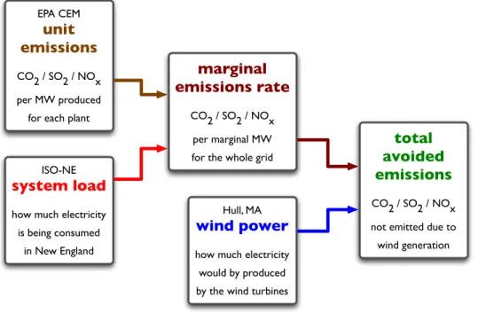
Overview
The AGREA avoided emissions methodology combines a number of disparate data sources— for clarity’s sake, here is an overview of how they all fit together:
EPA CEM
unit emissions
CO2 / SO2 / NOx per MW produced
for each plant
ISO-NE system load how much electricity is being consumed
in New England
marginal emissions rate
CO2 / SO2 / NOx per marginal MW for the whole grid
Hull, MA
wind power
how much electricity would by produced by the wind turbines
total avoided emissions CO2 / SO2 / NOx not emitted due to wind generation
First of all, we load the data from the sources described in the data section into
the database. As we load the EGRID fossil generating unit data, we also compute the following for each unit in each hour: the change in unit load, the unit’s load state,
and whether or not the unit’s is flagged as “Load Shape Following” (LSF). The basic algorithm is as follows: the unit’s change in load is simply the difference between the
output in each hour and the output in the hour preceding it.
To identify the load state, we first determine the unit’s maximum output in the cur-rent year and the two years preceding it. If the curcur-rent year is the first year of the
dataset, we look at the current year and one year ahead of it. We take this maximum output to be the unit’s operational capacity—the nameplate capacity (analogous to the
capacity of a computer hard drive), is not an accurate enough indicator of the actual operational capacity of the unit. In addition to this capacity, we also calculate yearly
summer capacities, based only on the data from May through September, as the opera-tional capacity of thermal power plants is reduced when air temperatures are higher. So
now that we have a maximum capacity, we calculate the unit’s output during each hour as a percentage of that maximum capacity, and use that percentage to bin the unit in
that hour into one of four “load states”, as shown in Table 2.1.
Load Condition Load State
in any hour in that hour
output < 5% capacity Turning on or off 5% ≤ output < load 55% Standby
55% ≤ output < 90% Spinning Reserve
90% ≤ output Full Load
Table 2.1: Unit Load States and Conditions
Finally, we determine if the unit is following the load. First of all, any units in
spinning reserve are considered to follow load, and so they are automatically flagged as such. Units in all other load states are also flagged as load shape following in each hour
if one of the following is true: either the unit’s load is changing in the same direction as the system’s load, or the unit was flagged as load shape following in the previous hour
past hour.
Thus, for each unit, for each hour, we have three new pieces of data: the change in
unit load, the unit’s load state, and whether or not it is following the system load (Load Shape Following, or LSF). We write these data back into the same table in which the
hourly unit emissions stored, and also store the hourly change in total system load into the total system load table. With this new data, we are now ready to calculate the ISO’s
hourly marginal emission rates.
To calculate the marginal emission rates in each hour, we take a weighted average of the emissions from units following the system load. It’s basically the marginal emissions
of the marginal generation. We do this as follows: in each hour, we take the rate of emissions (amount of emission in that hour divided by the unit’s electricity output) and
then weight it by the change in load of that unit with respect to the total change in load of all units that are following the load in that hour. We perform this calculation for each
of the three emissions in the data set: CO2, SO2, and NOx. This gives us three hourly
time series of marginal emissions rates, expressed as mass of compound emitted per unit
of electricity produced. X lsf CO2 load ∆unit load P lsf∆unit load
= hourly marginal emission rate (2.1)
Exclusion of unit-hours displaying anomalous emission rates due to
measure-ment lag
In calculating the marginal emissions, we exclude all emissions from qualifying units in the hours that those units’ average emissions exceed either 5 tons of CO2 per megawatt-hour,
or 100 pounds of NOx per megawatt hour. This serves to exclude a number of outlying
hours whose emission rates are physically impossible. We theorize that these
anoma-lous data points are the result of the emissions monitoring equipment being mounted downstream of the point at which the operating parameters of the unit are measured,
resulting in a lag between the measurements. Thus the emissions caused by burning fuel near the end of an hour may be measured and recorded in the next hour. This effect is
the emissions and power output of the unit will not vary from hour to hour.
Now that we’ve calculated the marginal emissions rates, it is fairly straightforward
to determine emissions avoided by the renewable generation. Since we assume that the electricity produced by the renewable generation can’t be stored, and thus must be used
in the same hour in which it was produced, emissions will be avoided at the marginal rate that we just computed. Thus, we simply multiply the hourly renewable electricity
production time series (expressed in MWh produced in each hour) by the marginal emis-sions rate (expressed in kilograms of compound emitted per MWh produced by fossil
generation in that hour) to give us the avoided emissions in that hour (expressed in mass of compound that was not emitted as a result of the renewable electricity production).
We actually calculate this using a nominal 1 MW installed capacity so that the results can be easily scaled to any size of installation under consideration. For example, to
com-pute the emissions avoided by a 12 MW installation of four 3 MW turbines, one simply multiplies the avoided emissions by 12. We conclude this historical analysis by recording
the time series of marginal emissions rates and total avoided emissions rates into the database so that they can be quickly accessed for further analysis.
2.4
Forward Looking Analysis
All of the above numerical gymnastics yields a strictly historical analysis. To project
the analysis into the future–to anticipate how many emissions might be avoided by a renewable generation project that is yet to be built–we proceed in two steps, separating
out insights on the emissions profile over the course of the day and year from the wind generation profile, and then recombining them to give us an anticipated range of avoided
emissions. First, we find the mean emissions rate for each season and time of day cohort, which gives us a new matrix of emissions rates for winter day, winter evening, and winter
nights, spring day, spring evening, spring nights, etc. Thus the first cell in the matrix contains the mean emissions rate for all winter daytime hours over all years in the dataset.
winter day spring day summerday autumnday
winter evening spring evening summerevening autumnevening winter night spring night summernight autumnnight
With the mean LSF emissions rate for each seasonal and time of day cohort in hand,
we turn to the wind resource to develop a range of typical wind years, subdivided into seasons and times of day. We start by determining the mean wind power for each season
in year. We then identify the minimum, median, and maximum of each season, so we know which winter had the highest wind, which winter had the lowest wind, and which
winter had the median wind. Once we identify those representative seasons, we record the mean wind power generated in each time of day cohort within those seasons. Thus,
we build three matrices representing the range (minimum, median, and maximum) of wind speeds that we anticipate in future years; each matrix contains 12 elements, one for
each season and time of day cohort.
Now that we have the typical emission rates, and a set of wind generation profiles that
covers the anticipated range of wind generation, we merely multiply the the latter by the former, multiply each cell of the resulting matrix by the number of hours in each cohort
in a year, and sum the resulting avoided emissions. Thus, we calculate the anticipated avoided emissions for a low wind year, for a medium wind year, and a high wind year.
This analysis is admittedly coarse, and relies to a great deal on the emissions profile of the grid remaining the same. This, along with other limitations is discussed in greater
detail in Section 2.6.
2.5
Representation of the Results of the Analysis to
Policymakers and to the Public
All of the above analysis yields a great deal of data, but the question now before us is:
how do we distill those numbers into meaningful insights, and how do we communicate those insights to decision-makers and the public? I answer this question by first
installation, and then I relate the avoided emissions insights to their existing knowledge
and interactions with the world.
2.5.1
Decision-makers
The first group I examine is the ostensible target audience of this analysis: those to
whom the Environmental Impact Report must be circulated as mandated by section 11.16 of the MEPA regulations. This group includes: the Massachusetts Department
of Environmental Protection, the Massachusetts Coastal Zone Management office, the Division of Marine Fisheries, and the Department of Public Health.[14] To these readers,
I am communicating the following:
• The range of emissions that we anticipate that the project will offset
• How that anticipated range compares with the historical range of emissions
• How and why our projections differ from the anticipated avoided emissions calcu-lated by the methodology prescribed by the Massachusetts Greenhouse Gas policy
• Why our methodology is more appropriate than the Massachusetts GHG policy’s for the purpose of evaluating wind generation
To accomplish these disparate goals, I construct two figures, each communicating two of the above messages. To display the range of anticipated emissions in comparison with
the historical range, I construct a coarse time series that that shows some of the seasonal dynamics, but is focused on the total annual emissions. Since the hourly time series of
avoided emissions is not of interest, and may in fact provide too much detail, I bin the emissions up by season. I then stack the seasons for each year, and display the consecutive
years in order. After the most recent year in our analysis, I show the anticipated range of avoided emissions, similarly binned by season. I demarcate the boundary between
the historical emissions and the anticipatory with a strong line, and label both regions appropriately. I then mark the historical range, and extend its boundaries down into
range. Thus, we have a relatively clear chart that shows our projections, and puts them
in the context of the historical range of avoided emissions had the wind turbines been in operation. All emissions on this chart are expressed in terms of quantity of CO2 avoided
per megawatt of installed capacity, so to calculate the total avoided emissions for a given configuration of wind turbines, the decision-maker simply multiplies the emission
numbers on the chart by the number of megawatts under consideration. This enables the
comparison of several different configurations, but at the expense of some computational complexity, so the anticipated range is calculated and displayed for the primary candidate
configuration.
2.5.2
Public
The residents of Hull, on the other hand, are not, for the most part, going to be nearly as interested in the exact amount of CO2, SO2, and NOxthat will be avoided by this project.
Nor are they going to be terribly interested in the temporal dynamics of the analysis. Instead, what they want to know is, “If these turbines get built, what does that mean in
terms of my (and my town’s) electricity usage? Plus, I’ve heard that a couple of different size turbines are being considered, so what’s the trade-off for the big turbines compared
to the small ones?” To answer these questions, I construct a table of plots. Across the top of the table, I have several candidate turbine configurations: the first, no new
turbines, just the existing Hull 1 & 2 output; 3 × 3MW turbines; 3 × 3.6MW turbines, 4 × 3MW turbines, 4 × 3.6 MW turbines. Each of these configurations is represented by
a diagram of the turbines, highlighting the relative turbine size and the total capacity. Each row beneath that header row represents a different measurement, expressed in terms
of the town’s current energy and emissions footprint. Thus, the first row is simply the annual generation, the second avoided CO2, and so on. The resulting chart, Figure 3-23
shows the residents of Hull how much of their emissions will be avoided for each of the candidate configurations, and puts that next to the currently avoided emissions for the
2.6
Limitations
The AGREA LSF avoided emissions approach has a number of limitations that are primarily driven by uncertainty about the future, lack of data, or restrictions on access
to data. Some of these limitations can be addressed through further analysis. I have identified the following primary limitations:
• Lack of access to hourly non-fossil generation data
• Lack of identification of the marginal units in the day-ahead, real-time, and ancil-lary services markets
• Uncertainty as to the fuel mix and emissions profile of the future grid
2.6.1
Lack of access to hourly non-fossil data
The EGRID data set is, by definition, comprised of emissions and generation data from
only those units that emit CO2, SO2, or NOx. This means that the operating parameters
of all nuclear, hydropower, and wind plants are not represented, nor are electricity imports
or exports. Since our analysis weights the marginal emissions produced by each unit by the total marginal fossil response to the system demand, and this response is assumed
to be the total response, there may be a component of responsive generation that is not captured.
Nuclear power plants will generally be generating at full capacity whenever they can, so the lack of access to data on their generation doesn’t generally affect our analysis.
However, nuclear plants do get taken offline periodically for routine maintenance, and this loss in generation capacity must be made up for by fossil units, which may create artifacts
in our emission rates when the fossil units respond to the reduced nuclear capacity instead of the system demand.
Hydroelectric plants comes in two basic flavors: run-of-the-river and reservoir.
Run-of-the-river hydroelectricity is very similar to wind and solar power, in that electricity is generated whenever the renewable resource (in this case, running river water) is available.
most profitable times, as long as the reservoir isn’t full. Since reservoir hydropower can
come online very quickly, it is often used in the ancillary services market to balance demand and supply of electric generation. Not having access to the hourly generation
profile of reservoir hydroelectric generation does adversely affect our analysis, as this generation does respond to load. However, this effect is mitigated by the relatively small
(<5%) proportion of reservoir hydroelectric generation capacity in New England.[11]
Run-of-the-river hydro can by considered alongside wind and solar—these renewable sources of electricity have no marginal costs, and are highly temporally variable, so they
generate whenever they can. All three of these generation types do, however, have known seasonal and diurnal patterns, so further analysis can and should be undertaken to
miti-gate their impact on our marginal analysis. Furthermore, they represent an even smaller proportion of the generative capacity in New England than does reservoir hydropower,
so the extent of their impact is limited.
Imports and exports of electricity across the grid boundary are an issue, as they are
included in the total system load data from ISO-NE, but are not captured in the EPA CEM dataset. This means that we don’t have a complete picture of the source of the
electricity that is serving the load at any point in time. Unfortunately, this limitation is more difficult to address than the missing hydro and nuclear generation, as ISO-NE
doesn’t have nearly as much information about which units are producing the electricity it imports.
Finally, there are a number of fossil plants that are exempt from reporting into the Continuous Emissions Monitoring program. These are units that burn low sulfur (¡ 0.05%
by weight), non-coal fuels for a total nameplate capacity of less than 25 megawatts.[4] I do not anticipate that the lack of data on these units will cause a significant adverse
2.6.2
Lack of identification of the marginal units in the
day-ahead, real-time, and ancillary services markets
Our analytical approach, and in particular our method of identifying the units that are responding to load in any particular hour, is based on the only data we have available
to us: the actual operating parameters of each unit in each hour. We know only how each unit is behaving; we don’t know why. Specifically, we don’t know what sorts of bids
the unit operators submitted to the day-ahead, realtime, and ancillary services markets, and which of those bids was accepted. As Connolly shows in his 2008 thesis,[8] plants
across the fuel spectrum bid into each of these markets. Since renewable electricity is produced at the rate at which the resource is available, it will likely be bidding into the
realtime market, and will thus avoid the emissions associated with the marginal bid in that market.
If we knew which unit the marginal bid was placed for in each hour, our analysis
would be more representative of the the actual behavior of the market. Unfortunately for us, while ISO-NE does provide a great deal of information about the bids submitted,
it does not identify the units that the bids are submitted for to prevent anticompetitive gaming of the market. While this is good for the economic performance of the market,
it does impair our ability to accurately quantify the avoided emissions from renewable generation. However, since ISO New England does have access to this data, it could, as
a part of preparing its annual Marginal Emissions Report, perform this analysis while still sufficiently obfuscating the original bid data to prevent collusion.
2.6.3
Uncertainty as to the fuel mix and emissions profile of
the future grid
The extension of our historical, marginal LSF analysis into the future raises a number of questions, chief among them: what fuels will generators be burning in the coming years,
and how much will they be emitting? While our historical analysis can give us some idea of the answers to these questions in the past, there are several exogenous factors that
Of the generating units currently online, the subset of those that are in operation
(and their level of output) at any time is determined primarily by the results of the the markets managed by ISO-New England. Since fossil units marginal costs (and thus their
bids into the various markets) are heavily dependent on fuel costs, a shift in the price of one fossil fuel relative to another can have immediate effects in the bidding behavior
of various plants, and the fuel mix of the set of dispatched plants could be affected as a
result.
Because the fossil fuels differ in their carbon intensity (unit of CO2emitted per unit of
electricity generated), changes in the fuel mix of the grid will be accompanied by changes
in the emissions rate of the grid. As more electricity is produced from coal relative to natural gas, more CO2 is emitted. The relative fuel prices can be affected by any number
of factors: their inherent volatility, supply constraints, seasonal variations in demand patterns, etc. Fossil fuel prices, especially those of oil and natural gas, are volatile in and
of themselves, and although their variability is somewhat correlated over the long term, in the short term the price of each fuel can jump without the other responding.
The Regional Greenhouse Gas Initiative, New England’s first try at a CO2
cap-and-trade system, will also affect operating costs of plants burning different fuels at different
rates, due to the variation in carbon intensities previously discussed. This will have the effect of raising the cost of burning all fossil fuels, and will cost coal plants approximately
1.2 times as much as oil plants, and 1.7 times as much as gas plants per kWh produced. Thus, one of RGGI’s potential effects will be to move coal units higher up in the
dis-patch queue. However, since cap-and-trade systems don’t actually set a price for carbon credits, the actual magnitude of RGGI’s effect on the economic dispatch of fossil units is
uncertain.
Finally, there may be legislative mandates that, given the existence of enabling
tech-nologies, restrict emissions in and of themselves. An example of this type of an effect is the precipitous drop in SO2 and NOx emissions due to the Clean Air Act. This drop can
be clearly seen in our historical analysis of these two emissions: emissions fell every year from 2000 to 2003, and stabilized thereafter. This drop was caused by the mandated
Congress decide to tighten the emission limits, we would expect to see a similar drop in
the future, if the technologies are capable of it. Unfortunately, there currently exist no economically viable technologies to scrub CO2out of the stacks, so until such technologies
Chapter 3
Results
3.1
Marginal Emission Rates
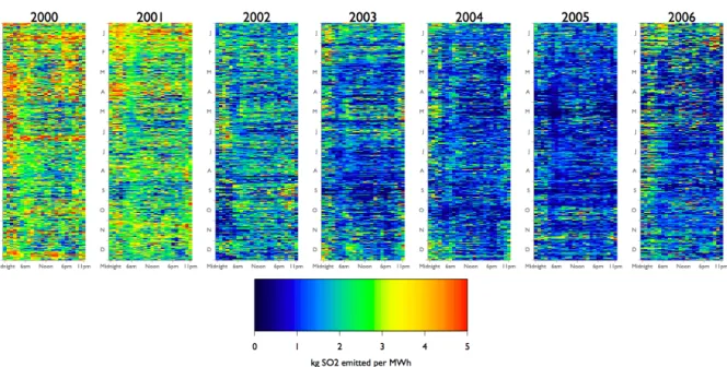
Utilizing the methodology described in the previous sections, I generated an hourly time series for the marginal emission rates in the New England grid for each of the following
compounds: CO2, SO2, and NOx. The full data set can be seen in the figures on the
following pages, in the form of a series of 8760 diagrams, so named because they display
each of the 8,760 hours in a year—the 24 hours in a day running across the horizontal axis, and the 365 days in a year descending the vertical axis. Thus, time-of-day patterns
can be seen as vertical stripes, whereas seasonal patterns show up as horizontal bands. As can be seen in the diagrams, there is a tremendous amount of variability in and between
the emission rates. Let’s examine the marginal emission rates for each compound, in turn, to explore some of these episodic patterns.
3.1.1
Marginal CO
2Emission Rates
The marginal emission rates for CO2 exhibit two patterns that are of interest to us.
First, there is a bimodal diurnal pattern, with a streak of high emission rates in the early
morning hours and late evening hours. This can be seen especially clearly in the 2005 8760, which has a yellow streak running down the left side, throughout the year, at around
Figure 3-1: Hourly Marginal CO2 Emission Rates
hkg CO
2
MWhr
i
or 10 o’clock in the evening. This diurnal pattern can also be seen in the hourly average chart in Figure 3-2; note the spike at 9pm. The other pattern is actually interesting in
its absence: there is a no discernible seasonal pattern—the summers look much like the winters. This makes the marginal emission rate of CO2, as I will demonstrate shortly,
the exception amongst the three compounds measured here.
Seasonal Marginal CO2 Emission Rates 1999 - 2006
A
verage marginal CO2 emission rate [kg/MWhr]
Jan Feb Mar Apr May Jun Jul Aug Sep Oct Nov Dec Jan
0 200 400 600 800 1000
Hourly Marginal CO2 Emission Rates 1999 - 2006
A
verage marginal CO2 emission rate [kg/MWhr]
Midnight 3am 6am 9am Noon 3pm 6pm 9pm
0 200 400 600 800 1000
Year-round Summer (April-September)
Winter (October-March)
3.1.2
Marginal SO
2Emission Rates
Figure 3-3: Hourly Marginal SO2 Emission Rates
hkg SO
2
MWhr
i
Seasonal Marginal SO2 Emission Rates 1999 - 2006
A
verage marginal SO2 emission rate [kg/MWhr]
Jan Feb Mar Apr May Jun Jul Aug Sep Oct Nov Dec Jan
0.0 0.5 1.0 1.5 2.0 2.5 3.0
Hourly Marginal SO2 Emission Rates 1999 - 2006
A
verage marginal SO2 emission rate
, kg/MWhr
Midnight 3am 6am 9am Noon 3pm 6pm 9pm
0.0 0.5 1.0 1.5 2.0 2.5 3.0 Year-round Summer (April-September) Winter (October-March)
Figure 3-4: Hourly Marginal SO2 Emissions – Seasonal and Diurnal Trends
In contrast to CO2, the marginal SO2 emission rates show far more than simply a
diurnal pattern. The first thing that jumps out is the drastic decrease in emission rates
from 2000 through 2003. Besides that inter-annual trend, we also see a seasonal pattern that peaks at around 2.8 kg SO2
MWhr a peak in December and drops to a low of around 2.1
kg SO2
and hitting its low at around 6pm. The diurnal pattern’s peak and zenith don’t vary
that much over the course of the year, but there is a decent gap between the summer and winter average in the intervening hours.
3.1.3
Marginal NO
XEmission Rates
Figure 3-5: Hourly Marginal NOX Emission Rates
hkg NO
x
MWhr
i
Seasonal Marginal NOx Emission Rates 1999 - 2006
A
verage marginal NOx emission rate [kg/MWhr]
Jan Feb Mar Apr May Jun Jul Aug Sep Oct Nov Dec Jan
0.0 0.2 0.4 0.6 0.8 1.0
Hourly Marginal NOx Emission Rates 1999 - 2006
A
verage marginal NOx emission rate
, kg/MWhr
Midnight 3am 6am 9am Noon 3pm 6pm 9pm
0.0 0.2 0.4 0.6 0.8 1.0 Year-round Summer (April-September) Winter (October-March)
Figure 3-6: Hourly Marginal NOx Emissions – Seasonal and Diurnal Trends