HAL Id: hal-01007706
https://hal.archives-ouvertes.fr/hal-01007706
Submitted on 17 Jun 2014
HAL is a multi-disciplinary open access
archive for the deposit and dissemination of
sci-entific research documents, whether they are
pub-lished or not. The documents may come from
teaching and research institutions in France or
abroad, or from public or private research centers.
L’archive ouverte pluridisciplinaire HAL, est
destinée au dépôt et à la diffusion de documents
scientifiques de niveau recherche, publiés ou non,
émanant des établissements d’enseignement et de
recherche français ou étrangers, des laboratoires
publics ou privés.
Two Recursively Inseparable Problems for Probabilistic
Automata
Nathanaël Fijalkow, Hugo Gimbert, Florian Horn, Youssouf Oualhadj
To cite this version:
Nathanaël Fijalkow, Hugo Gimbert, Florian Horn, Youssouf Oualhadj. Two Recursively Inseparable
Problems for Probabilistic Automata. MFCS 2014, Aug 2014, Budapest, Hungary. Paper 168.
�hal-01007706�
Two Recursively Inseparable Problems
for Probabilistic Automata
⋆Nathana¨el Fijalkow1,2, Hugo Gimbert3, Florian Horn1, and Youssouf Oualhadj4
LIAFA, Universit´e Paris 7, France, University of Warsaw, Poland, LaBRI, Universit´e de Bordeaux, France,
Universit´e de Mons, Belgium.
Abstract. This paper introduces and investigates decision problems for
numberlessprobabilistic automata, i.e. probabilistic automata where the
supportof each probabilistic transitions is specified, but the exact values of the probabilities are not. A numberless probabilistic automaton can be instantiated into a probabilistic automaton by specifying the exact values of the non-zero probabilistic transitions.
We show that the two following properties of numberless probabilistic automata are recursively inseparable:
• all instances of the numberless automaton have value 1, • no instance of the numberless automaton has value 1.
1
Introduction
In 1963 Rabin [12] introduced the notion of probabilistic automata, which are fi-nite automata able to randomise over transitions. A probabilistic automaton has a finite set of control states Q, and processes finite words; each transition consists in updating the control state according to a given probabilistic distribution de-termined by the current state and the input letter. This powerful model has been widely studied and has applications in many fields like software verification [3], image processing [5], computational biology [6] and speech processing [10].
Several algorithmic properties of probabilistic automata have been consid-ered in the literature, sometimes leading to efficient algorithms. For instance, functional equivalence is decidable in polynomial time [13,14], and even faster with randomised algorithms, which led to applications in software verification [9]. However, many natural decision problems are undecidable, and part of the literature on probabilistic automata is about intractability results. For example the emptiness, the threshold isolation and the value 1 problems are undecid-able [11,2,8].
A striking result due to Condon and Lipton [4] states that, for every ǫ > 0, the two following problems are recursively inseparable: given a probabilistic automaton A,
⋆
The research leading to these results has received funding from the European Union’s Seventh Framework Programme (FP7/2007-2013) under grant agreement no
259454 (GALE) and from the French Agence Nationale de la Recherche projects EQINOCS (ANR-11-BS02-004) and STOCH-MC (ANR-13-BS02-0011-01).
• does A accept some word with probability greater than 1 − ε? • does A accept every word with probability less than ε?
In the present paper we focus on numberless probabilistic automata, i.e. prob-abilistic automata whose non-zero probprob-abilistic transitions are specified but the exact values of the probabilities are not. A numberless probabilistic automaton can be instantiated into a probabilistic automaton by specifying the exact values of the non-zero probabilistic transitions (see Section 2 for formal definitions).
The notion of numberless probabilistic automaton is motivated by the fol-lowing example. Assume we are given a digital chip modelled as a finite state machine controlled by external inputs. The internal transition structure of the chip is known but the transitions themselves are not observable. We want to compute an initialisation input sequence that puts the chip in a particular ini-tial state. In case some of the chip components have failure probabilities, this can be reformulated as a value 1 problem for the underlying probabilistic automa-ton: is there an input sequence whose acceptance probability is arbitrarily close to 1? Assume now that the failure probabilities are not fixed a priori but we can tune the quality of our components and choose the failure probabilities, for instance by investing in better components. Then we are dealing with a number-less probabilistic automaton and we would like to determine whether it can be instantiated into a probabilistic automaton with value 1, in other words we want to solve an existential value 1 problem for the numberless probabilistic automa-ton. If the failure probabilities are unknown then we are facing a second kind of problem called the universal value 1 problem: determine whether all instances of the automaton have value 1. We also consider variants where the freedom to choose transition probabilities is restricted to some intervals, that we call noisy value 1 problems.
One may think that relaxing the constraints on the exact transition proba-bilities makes things algorithmically much easier. However this is not the case, and we prove that the existential and universal value 1 problems are recursively inseparable: given a numberless probabilistic automaton C,
• do all instances of C have value 1? • does no instance of C have value 1?
This result is actually a corollary of a generic construction which constitutes the technical core of the paper and has the following properties. For every simple probabilistic automaton A, we construct a numberless probabilistic automaton C such that the three following properties are equivalent:
(i) A has value 1,
(ii) one of the instances of C has value 1, (iii) all instances of C have value 1.
The definitions are given in Section 2. The main technical result appears in Section 3, where we give the generic construction whose properties are described
above. In Section 4, we discuss the implications of our results, first for the noisy value 1 problems, and second for probabilistic B¨uchi automata [1].
2
Definitions
Let A be a finite alphabet. A (finite) word u is a (possibly empty) sequence of letters u = a0a1· · · an−1; the set of finite words is denoted by A∗.
A probability distribution over a finite set Q is a function δ : Q → Q≥0 such
thatPq∈Qδ(q) = 1; we denote by 13· q +23· q′ the distribution that picks q with
probability 13 and q′with probability 23, and by q the trivial distribution picking q with probability 1. The support of a distribution δ is the set of states picked with positive probability, i.e., supp(δ) = {q ∈ Q | δ(q) > 0}. Finally, the set of probability distributions over Q is D(Q).
Definition 1 (Probabilistic automaton). A probabilistic automaton (PA) is a tuple A = (Q, A, q0, ∆, F ), where Q is a finite set of states, A is the finite
input alphabet, q0∈ Q is the initial state, ∆ : Q × A → D(Q) is the probabilistic
transition function, and F ⊆ Q is the set of accepting states.
For convenience, we also use PA(s−→ t) to denote the probability of goingu
from the state s to the state t reading u, PA(s−→ S) to denote the probabilityu
of going from the state s to a state in S reading u, and PA(u), the acceptance
probability of a word u ∈ A∗, to denote P
A(q0−→ F ).u
We often consider the case of simple probabilistic automata, where the tran-sition probabilities can only be 0,1/2, or 1.
Definition 2 (Value). The value of a PA A, denoted val(A), is the supremum acceptance probability over all input words
val(A) = sup
u∈A∗
PA(u) .
The value 1 problem asks, given a (simple) PA A as input, whether val(A) = 1. Theorem 1 ([8]). The value 1 problem is undecidable for simple PA.
Definition 3 (Numberless probabilistic automaton). A numberless prob-abilistic automaton (NPA) is a tuple A = (Q, A, q0, T, F ), where Q is a finite set
of states, A is the finite input alphabet, q0∈ Q is the initial state, T ⊆ Q× A× Q
is the numberless transition function, and F ⊆ Q is the set of accepting states. The numberless transition function T is an abstraction of probabilistic tran-sition functions. We say that ∆ is consistent with T if for all letters a and states s and t, ∆(s, a, t) > 0 if, and only if (s, a, t) ∈ T .
A numberless probabilistic automaton is an equivalence class of probabilis-tic automata, which share the same set of states, input alphabet, initial and accepting states, and whose transition functions have the same support.
A NPA A = (Q, A, q0, T, F ) together with a probabilistic transition function
∆ consistent with T defines a PA A[∆] = (Q, A, q0, ∆, F ). Conversely, a PA
A = (Q, A, q0, ∆, F ) induces an underlying NPA [A] = (Q, A, q0, T, F ), where
T ⊆ Q × A × Q is defined by (q, a, p) ∈ T if ∆(q, a)(p) > 0. We consider two decision problems for NPA:
– The existential value 1 problem: given a NPA A, determine whether there exists ∆ such that val(A[∆]) = 1.
– The universal value 1 problem: given a NPA A, determine whether for all ∆, we have val(A[∆]) = 1.
Proposition 1. There exists a NPA such that: – there exists ∆ such that val(A[∆]) = 1, – there exists ∆′ such that val(A[∆′]) < 1.
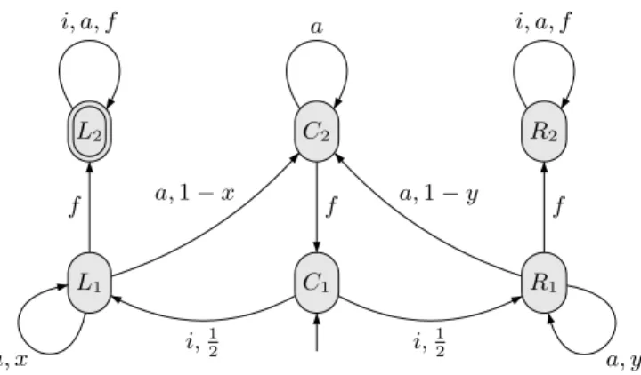
C1 C2 L1 L2 R1 R2 a f i,1 2 a, 1 − x f a, x i, a, f i,1 2 a, 1 − y f a, y i, a, f
Fig. 1.This NPA has value 1 if and only if x > y
In this automaton, adapted from [8,7], the shortest word that can be accepted is i · f , as i goes from C1 to L1, and f goes from L1 to L2. However, there are
as much chances to go to R2, so the value of i · f is1/2.
If x is strictly less than y, one can tip the scales to the left by adding a’s between the i and f : each time, the run will have more chances to stay left than to stay right. After reading i · an· f , the probability of reaching L
2 is equal to
xn, while the probability of reaching R
2 is only yn. There is also a very high
chance that the run went back to C1, but from there we can simply repeat our
word an arbitrary number of times.
Let x, y, and ε be three real numbers such that 0 ≤ y < x ≤ 1, and 0 < ε ≤ 1. There is an integer n such thatxn
/(xn
+yn
)is greater than 1 −ε/2, and an integer
m such that (1 − xn− yn)m
is less thanε/2. The word (i · an· f )m
is accepted with probability greater than 1 − ε.
3
Recursive inseparability for numberless value 1
problems
In this section, we prove the following theorem:
Theorem 2. The two following problems for numberless probabilistic automata are recursively inseparable:
– all instances have value 1, – no instance has value 1.
Recall that two decision problems A and B are recursively inseparable if their languages LA and LB of accepted inputs are disjoint and there exists no
recursive language L such that LA⊆ L and L ∩ LB= ∅.
Note that it implies that both A and B are undecidable.
Equivalently, this means there exists no terminating algorithm which has the following behaviour on input x:
– if x ∈ LA, then the algorithm answers “YES”
– if x ∈ LB, then the algorithm answers “NO”.
On an input that belongs neither to LA nor to LB, the algorithm’s answer can
be either “YES” or “NO”.
3.1 Overall construction
Lemma 1. There exists an effective construction which takes as input a simple PA A and constructs a NPA C such that
val(A) = 1 ⇐⇒ ∀∆, val(C[∆]) = 1 ⇐⇒ ∃∆, val(C[∆]) = 1 .
We first explain how Lemma 1 implies Theorem 2. Assume towards contra-diction that the problems “all instances have value 1” and “no instance has value 1” are recursively separable. Then there exists an algorithm A taking a NPA as input and such that: if all instances have value 1, then it answers “YES”, and if no instance has value 1, then it answers “NO”. We show using Lemma 1 that this would imply that the value 1 problem is decidable for simple PA, contradicting Theorem 1. Indeed, let A be a simple PA, applying the construction yields a NPA C such that
val(A) = 1 ⇐⇒ ∀∆, val(C[∆]) = 1 ⇐⇒ ∃∆, val(C[∆]) = 1 .
In particular, either all instances of C have value 1, or no instance of C has value 1. Hence, if it answers “YES” then val(A) = 1 and it if answers “NO” then val(A) < 1, allowing to decide whether A has value 1 or not. This concludes the proof of Theorem 2 assuming Lemma 1.
The first step is to build from A a family of PA’s Bλ whose transitions are
all of the form q−→ (λ · r, (1 − λ) · s) in such a way that Ba λ has the same value
as A for any value of λ. Note that, while all the Bλ’s belong to the same NPA,
they are not, in general, a NPA: for example, if A were the simple version of the automaton of Figure 1, the Bλ’s would be the instances where x = y = λ, while
the underlying NPA would also include the cases where x 6= y.
The second step is to build from the Bλ’s a NPA C such that, for each
probabilistic transition function ∆, there is a λ such that C[∆] has value 1 if, and only if Bλhas value 1.
It follows that:
∃∆, val(C[∆]) = 1 =⇒ ∃λ, val(Bλ) = 1
=⇒ val(A) = 1 =⇒ ∀λ, val(Bλ) = 1
=⇒ ∀∆, val(C[∆]) = 1 .
3.2 The fair coin construction
Let A = (Q, A, q0, ∆, F ) be a simple PA over the alphabet A. We construct a
family of PAs (Bλ)λ∈]0,1[ over the alphabet B = A ∪ {♯}, whose transitions have
probabilities 0, λ, 1 − λ or 1, as follows.
The automaton Bλis a copy of A where each transition of A is replaced by the
gadget illustrated in Figure 2 (for simplicity, we assume that all the transitions of A are probabilistic). The initial and final states are the same in A and Bλ.
The left hand side shows part of automaton A: a probabilistic transition from q reading a, leading to r or s each with probability half. The right hand side shows how this behaviour is simulated by Bλ: the letter a leads to an intermediate
state qa, from which we can read a new letter ♯. Each time a pair of ♯’s is read,
the automaton Bλgoes to r with probability λ·(1−λ), goes to s with probability
(1 − λ) · λ, and stays in qa with probability λ2+ (1 − λ)2. Reading a letter other
than ♯ while the automata is still in one of the new states leads to the new sink state ⊥, which is not accepting. Thus, the probability of going to r is equal to the probability of going to s, and we can make the probability of a simulation failure as low as we want by increasing the number of ♯’s between two successive “real” letters.
Let u be a word of A∗. We denote by [u]k the word of B∗ where each letter
a ∈ A of u is replaced by a · ♯2k. Conversely, if w is a word of B∗, we denote by
˜
w the word obtained from w by removing all occurrences of the letter ♯. Intuitively, a run of A on the word u is simulated by a run of Bλ on the
word [u]k. Whenever there is a transition in A, B
λmakes k attempts to simulate
it through the gadget of Figure 2, and each attempt succeeds with probability (1 − 2λ · (1 − λ)), so each transition fails with probability:
Aλ,k= 1 − (1 − 2λ · (1 − λ))k .
q r s a,1 2 a,1 2 q qa qa, L qa, R r s ⊥ ♯ a ♯, λ ♯, 1 − λ ♯, 1 − λ ♯, λ ♯ ♯ A A A A ∪ {♯}
Fig. 2.The fair coin gadget.
1. For all q, r ∈ Q, a ∈ A, and k ∈ N, PBλ(q
[a]k
−−→ r) = Aλ,k· PA(q−→ r) ,a
2. For all q, r ∈ Q, u ∈ A∗, and k ∈ N, P Bλ(q
[u]k
−−→ r) = A|u|λ,k· PA(q−→ r) .u
3. For all q, r ∈ Q, w ∈ (A ∪ {♯})∗, and k ∈ N, P Bλ(q w −→ r) ≤ PA(q ˜ w −→ r) . It follows from Proposition 2 that for any λ, the value of Bλ is equal to the
value of A.
3.3 The simulation construction
All the Bλ’s induce the same NPA, that we denote by B. The problem is that
there are many other instances of B, whose values may be higher than the value of A (recall the example of Figure 1, where the Bλ have value1/2, while there
are instances of B with value 1). In this subsection, we construct a NPA C (over an extended alphabet C) whose instances simulate all the Bλ’s, but only them.
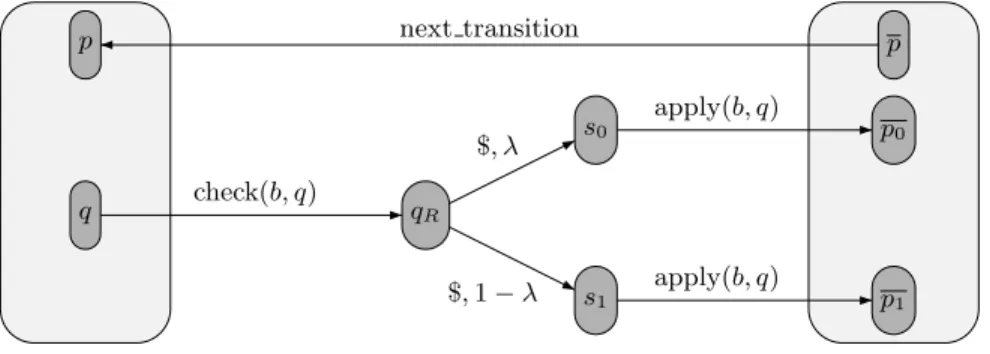
The idea is that the new NPA should only have one probabilistic transition. An instance of this transition translates to a value for λ. Figure 3 describes a first attempt at this (notice that our convention is that an non-drawn transition means a loop, rather than a transition to a sink state).
p q qR s0 s1 p p0 p1 next transition check(b, q) $, λ $, 1 − λ apply(b, q) apply(b, q)
In this automaton, that we call B′, there are two copies of the set of states,
and a single shared probabilistic transition qR $
−
→ (λ·s0, (1−λ)·s1) between them.
In order to make all the probabilistic transitions of B happen in this center area, we use new letters to detect where the runs come from before the probabilistic transition, and where it should go afterwards.
For each pair of a letter b in B and a state q in Q, we introduce two new letters check(b, q) and apply(b, q). The letter check(b, q) loops over each state except the left copy of q, which goes to qR. The letter apply(b, q) loops over each
state except s0, from where it goes to the λ-valued successor of (q, b) in Bλ, and
s1, from where it goes to the (1 − λ)-valued successor of (q, b) in Bλ. The new
letter next transition sends the run back to the left part once each possible state has been tested.
Thus, if we define the morphismb by its action on letters:
bb = check(b, q0)·$·apply(b, q0) · · · check(b, qn−1)·$·apply(b, qn−1)·next transition ,
where the qi’s are the states of Bλ, we get for any word u on the alphabet B,
PBλ(u) = PB′λ(bu).
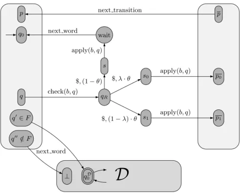
The problem with this automaton is that one can “cheat”, either by not testing an unwelcome state, or by changing state and letter between a check and the subsequent apply. In order to avoid this kind of behaviour, we change the automaton so that it is necessary to win an arbitrarily large number of successive times in order to approach the value 1, and we can test whether the word is fair after the first successful attempt. A side effect is that the simulation only works for the value 1: for other values, it might be better to cheat. The resulting automaton is described in Figure 4.
The structure of the automaton of Figure 3 is still there, but it has been augmented with an extra layer of scrutiny: each time we use the probabilistic transition, there is now a positive probability (1 − θ) to go to a new wait state. There is also a new letter next word which has the following effect:
– if the run is in an accepting state, it goes to the initial state of the fairness checker D;
– if the run is in a non-accepting state, it goes to the non-accepting sink state ⊥ of D;
– if the run is in the wait state, it goes back to the initial state.
The fairness checker D is a deterministic automaton which accepts the lan-guage {bu · next word | u ∈ B∗}∗. Its final state is the only final state in all of
C.
Intuitively, a run can still cheat before the first next word letter, but the benefits of doing so are limited: the probability that C[λ, θ] accepts a word at that point is at most θ (except if the empty word is accepting, but that case is trivial). After that point, cheating is risky: if the run already reached D, a false move will send it to the sink.
A more formal proof follows. A simple inspection of the construction of C yields Proposition 3:
D
p q0 q q′∈ F q′′∈ F/ wait s qR s0 s1 p p0 p1 ⊥ qD 0 next transition check(b, q) next word next word $, λ · θ $, (1 − λ) · θ $, (1 − θ) apply(b, q) apply(b, q) apply(b, q)Fig. 4.The Numberless Probabilistic Automaton C.
Proposition 3. Let u be a word of B∗ of length k. We have:
PC[λ,θ](u · next word) = θb k· PBλ(u)
PC[λ,θ]((u · next word)b ℓ) = (1 − (1 − θk)ℓ) · PBλ(u) .
It follows from Proposition 3 that the value of C[λ, θ] is at least the value of Bλ.
Proposition 4. Let u be a word of (C \ {next word})+. We have:
PC[λ,θ](u) ≤ θ .
Proposition 5 formalises the fact that there is no point in cheating after the first next word letter:
Proposition 5. Let u1, . . . , uk be k words of (C \ {next word})∗ and w be the
word u1· next word · · · uk· next word. Then, for any 1 ≤ i ≤ k, if ui ∈ c/ B∗, we
have:
PC[λ,θ](w) ≤ PC[λ,θ](ui· next word · · · uk· next word) .
Proof. After reading u1· · · ui−1·next word, a run must be in one of the following
three states: q0, q0D, and ⊥. As ui∈ c/B∗, reading it from q0Dwill lead to ⊥. Thus,
PC[λ,θ](w) = PC[λ,θ](q0
u1···ui−1·next word
−−−−−−−−−−−−→ q0) · PC[λ,θ](ui· · · uk· next word) ,
Finally, Proposition 6 shows that C[λ, θ] cannot have value 1 if Bλ does not.
Proposition 6. For all words w ∈ C∗ such that P
C[λ,θ](w) > θ, there exists a
word v ∈ B∗ such that
PBλ(u) ≥
PC[λ,θ](w) − θ 1 − θ .
Proof. Let us write w = u1· next word · · · uk· next word with u1, . . . , uk∈ (C \
{next word})∗. By Proposition 4, k > 1, and by Proposition 5 we can assume
that u2, . . . , ukbelong to cB∗. Let v2, . . . , vkbe the words of B∗such that ui=vbi.
The C[λ, θ]-value of w can be seen as a weighted average of 1 (the initial cheat, with a weight of θ) and the Bλ values of the vi’s (the weight of PBλ(vi) is the
probability that the run enters D while reading ui). It follows that at least one
of the vi’s has a Bλ-value greater than the C[λ, θ]-value of w
Thus, for each λ and θ, the value of C[λ, θ] is 1 if and only if the value of Bλ
is 1. As all the Bλ’s have the same value, which is equal to the value of A, we
get: ∃∆, val(C[∆]) = 1 =⇒ ∃λ, val(Bλ) = 1 =⇒ val(A) = 1 =⇒ ∀λ, val(Bλ) = 1 =⇒ ∀∆, val(C[∆]) = 1 . Theorem 2 follows.
4
Consequences
In this section, we show several consequences of the recursive inseparability re-sults from Theorem 2 and of the construction from Lemma 1. The first is a series of undecidability results for variants of the value 1 problem. The second is about probabilistic B¨uchi automata with probable semantics, as introduced in [1].
4.1 The noisy value 1 problems
Observe that Theorem 2 implies the following corollary:
Corollary 1. Both the universal and the existential value 1 problems are unde-cidable.
We can go further. Note that the universal and existential value 1 problems quantify over all possible probabilistic transition functions. Here we define two more realistic problems for NPA, where the quantification is restricted to prob-abilistic transition functions that are ε-close to a given probprob-abilistic transition function:
– The noisy existential value 1 problem: given a NPA A, a probabilistic transition function ∆ and ε > 0, determine whether there exists ∆′ such
– The noisy universal value 1 problem: given a NPA A, a probabilistic transition function ∆ and ε > 0, determine whether for all ∆′ such that
|∆′− ∆| ≤ ε, we have val(A[∆′]) = 1.
It follows from Lemma 1 that both problems are undecidable:
Corollary 2. Both the noisy universal and the noisy existential value 1 problems are undecidable.
Indeed, we argue that the construction from Lemma 1 implies a reduction from either of these problems to the value 1 problem for simple PA, hence the undecidability. Let A be a simple PA, the construction yields a NPA C such that:
val(A) = 1 ⇐⇒ ∀∆, val(C[∆]) = 1 ⇐⇒ ∃∆, val(C[∆]) = 1 .
It follows that for any probabilistic transition function ∆ and any ε > 0, we have:
val(A) = 1 ⇐⇒ (∀∆′, |∆′− ∆| ≤ ε =⇒ val(C[∆′]) = 1)
⇐⇒ (∃∆′, |∆′− ∆| ≤ ε ∧ val(C[∆′]) = 1) .
This completes the reduction.
4.2 Probabilistic B¨uchi automata with probable semantics
We consider PA over infinite words, as introduced in [1]. A probabilistic B¨uchi automaton (PBA) A can be equipped with the so-called probable semantics, defining the language (over infinite words):
L>0(A) = {w ∈ Aω| PA(w) > 0} .
It was observed in [1] that the value 1 problem for PA (over finite words) easily reduces to the emptiness problem for PBA with probable semantics (over infinite words).
Informally, from a PA A, construct a PBA A′ by adding a transition from
every final state to the initial state labelled with a new letter ♯. (From a non-final state, the letter ♯ leads to a rejecting sink.) As explained in [1], this simple construction ensures that A has value 1 if and only if A′is non-empty, equipped
with the probable semantics.
This simple reduction, together with Theorem 2, implies the following corol-lary:
Corollary 3. The two following problems for numberless PBA with probable semantics are recursively inseparable:
– all instances have a non-empty language, – no instance has a non-empty language.
Acknowledgments
References
1. Christel Baier, Nathalie Bertrand, and Marcus Gr¨oßer. Probabilistic ω-automata.
Journal of the ACM, 59(1):1, 2012.
2. Alberto Bertoni, Giancarlo Mauri, and Mauro Torelli. Some recursive unsolvable problems relating to isolated cutpoints in probabilistic automata. In International
Colloquium on Automata, Languages and Programming, pages 87–94, 1977. 3. Krishnendu Chatterjee, Laurent Doyen, Thomas A. Henzinger, and Jean-Fran¸cois
Raskin. Algorithms for omega-regular games of incomplete information. Logical
Methods in Computer Science, 3(3), 2007.
4. Anne Condon and Richard J. Lipton. On the complexity of space bounded in-teractive proofs (extended abstract). In Foundations of Computer Science, pages 462–467, 1989.
5. Karel Culik and Jarkko Kari. Digital images and formal languages, pages 599–616. Springer-Verlag New York, Inc., 1997.
6. Richard Durbin, Sean R. Eddy, Anders Krogh, and Graeme Mitchison. Biological
Sequence Analysis: Probabilistic Models of Proteins and Nucleic Acids. Cambridge University Press, July 1999.
7. Nathana¨el Fijalkow, Hugo Gimbert, and Youssouf Oualhadj. Deciding the value 1 problem for probabilistic leaktight automata. In Logics in Computer Science, pages 295–304, 2012.
8. Hugo Gimbert and Youssouf Oualhadj. Probabilistic automata on finite words: Decidable and undecidable problems. In International Colloquium on Automata,
Languages and Programming, pages 527–538, 2010.
9. Stefan Kiefer, Andrzej S. Murawski, Jo¨el Ouaknine, Bj¨orn Wachter, and James Worrell. Language equivalence for probabilistic automata. In Ganesh Gopalakr-ishnan and Shaz Qadeer, editors, CAV, volume 6806 of Lecture Notes in Computer
Science, pages 526–540. Springer, 2011.
10. Mehryar Mohri. Finite-state transducers in language and speech processing.
Com-putational Linguistics, 23:269–311, June 1997.
11. Azaria Paz. Introduction to probabilistic automata. Academic Press, 1971. 12. Michael O. Rabin. Probabilistic automata. Information and Control, 6(3):230–245,
1963.
13. Marcel-Paul Sch¨utzenberger. On the definition of a family of automata.
Informa-tion and Control, 4, 1961.
14. Wen-Guey Tzeng. A polynomial-time algorithm for the equivalence of probabilistic automata. SIAM Journal on Computing, 21(2):216–227, 1992.