HAL Id: hal-01404826
https://hal-univ-paris.archives-ouvertes.fr/hal-01404826
Submitted on 29 Nov 2016
HAL is a multi-disciplinary open access
archive for the deposit and dissemination of
sci-entific research documents, whether they are
pub-lished or not. The documents may come from
teaching and research institutions in France or
abroad, or from public or private research centers.
L’archive ouverte pluridisciplinaire HAL, est
destinée au dépôt et à la diffusion de documents
scientifiques de niveau recherche, publiés ou non,
émanant des établissements d’enseignement et de
recherche français ou étrangers, des laboratoires
publics ou privés.
Transverse single-file diffusion near the zigzag transition
Jean-Baptiste Delfau, Christophe Coste, Michel Saint-Jean
To cite this version:
Jean-Baptiste Delfau, Christophe Coste, Michel Saint-Jean. Transverse single-file diffusion near the
zigzag transition. Physical Review E : Statistical, Nonlinear, and Soft Matter Physics, American
Physical Society, 2013, 87, pp.32163 - 32163. �10.1103/PhysRevE.87.032163�. �hal-01404826�
PHYSICAL REVIEW E87, 032163 (2013)
Transverse single-file diffusion near the zigzag transition
Jean-Baptiste Delfau, Christophe Coste, and Michel Saint JeanLaboratoire “Mati`ere et Syst`emes Complexes” (MSC), UMR 7057 CNRS, Universit´e Paris 7 Diderot, 75205 Paris Cedex 13, France (Received 7 February 2013; published 29 March 2013)
We study with numerical simulations the transverse fluctuations in quasi-one-dimensional systems of particles in a thermal bath, near the zigzag transition. We show that close to the zigzag threshold, the transverse fluctuations exhibit an anormal diffusion, characterized by a mean square displacement that increases as the square root of time. In contrast with the longitudinal fluctuations, this behavior of the transverse fluctuations cannot be explained by the single-file ordering. We provide an analytical modelization, and in the thermodynamic limit we demonstrate the existence of this subdiffusive regime near the zigzag transition, showing that it results from overdamped collective modes of the system. These calculations are extended to finite systems, in excellent agreement with the simulations data. We also exhibit some effects of the thermal fluctuations on the zigzag transition, and analyze them in the light of stochastic bifurcation theory.
DOI:10.1103/PhysRevE.87.032163 PACS number(s): 05.40.−a, 66.10.cg, 02.30.Oz I. INTRODUCTION
When biologists observed subdiffusive behaviors of molecules through cell membranes [1], the basic idea of the single-file diffusion (SFD) was that particles confined in quasi-one-dimensional (1D) geometries, in such a way that they cannot cross each other’s, will undergo anomalous diffusion. The first theoretical approaches have considered hard-core interactions between particles ordered along a line [2]. A non-Fickian diffusion is indeed demonstrated, with a longitudinal mean square displacement (MSD) scaling as the square root of time in the thermodynamic limit. This result has been extended to more realistic models with finite (nonzero) range interactions [3–6] and with finite numbers of particles [7–11]. The SFD has been observed in experiments [12–15], and in numerical simulations [5,16–18].
In Ref. [5], we described the longitudinal fluctuations of the particles by linearizing the equations of motion near their equilibrium positions. The resulting equations are those of a chain of masses and springs in a thermal bath, and the relevant coupled Langevin equations may be solved by a projection onto the normal modes of vibration of the chain. In the thermodynamic limit, we demonstrated that the longitudinal MSD behaves like ⟨!x2⟩ = F t1/2at long times. We found the
same expression for the mobility F as in overdamped systems [3,4,6], extending this result to underdamped systems as well. This is due to the fact that whatever the dissipation, provided it is finite (nonzero), there is always a finite band of overdamped modes near the zero frequency one [5]. Forfinite systems with
periodic boundary conditions, the long times behavior is the collective ordinary diffusion of an effective particle of mass that of the whole system. Nevertheless, a SFD regime is also observed at intermediate times. We emphasize the relevance of the zero frequency mode linked to the translational invariance to those two regimes.
When the amplitude of the transverse confinement potential is much greater than the characteristic interparticle energy, the minimum of energy is reached when all particles are aligned along the x axis. If the strength of the transverse potential is progressively decreased, it becomes eventually energetically favorable for the particles to move alternately away from the longitudinal axis, compensating the energy increase in the
transverse direction by the interaction energy decrease due to a larger interparticle distance between nearest neighbors. This configurational phase transition is known as the zigzag transition and is schematically displayed in Fig.1. It has been observed with ions in Paul’s trap [19–25] and with plasma dusts [26–29]. It has also been the subject of many numerical and analytical studies [24,30–39]. For trapped ions the interparticle interaction is given by a Coulomb potential, whereas for plasma dust it is given by a screened Yukawa potential, but whatever the considered interaction the phenomenology of the zigzag transition is basically the same.
The zigzag transition is a purely mechanical configurational phase transition, and may be described as a supercritical (or normal) pitchfork bifurcation [40,41] that happens at a critical value βzz of the transverse stiffness, the zigzag pattern being
established for β < βzz. Exactly at the transition, the restoring
force for the alternate transverse motions of the particles vanishes, so that a soft mode of null frequency appears. This is an example of the critical slowing down which is a typical feature of supercritical pitchfork bifurcations [41]. As was done in Ref. [5] for the longitudinal fluctuations, we describe the transverse fluctuations in terms of the dynamics of the transverse oscillation modes of the particles chain. The key results of this paper are the observation of a transverse SFD regime in numerical simulations and its theoretical explanation. The soft mode linked to the zigzag transition plays, for the transverse fluctuations, the same role as the translationally invariant mode for longitudinal fluctuations because both are of null frequency. It will explain in the same way the transverse SFD behavior.
Our system is submitted to a thermal bath, and the precise analysis of the time evolution of the transverse MSD sheds light on some effects relevant to stochastic bifurcations theory [42–47]. The diagram of a noisy bifurcation is blurred with respect to that of a purely deterministic bifurcation, so that the singularity at the threshold has to be replaced by abifurcation region [43,45,47]. We will show that our simulation results may be interpreted in these terms. In a further publication [48], we will consider more thoroughly the thermal effects on the zigzag transition.
This paper is organized as follows. The zigzag transition is characterized in Sec.II. Then the simulation method and the
TRANSVERSE SINGLE-FILE DIFFUSION NEAR THE . . . PHYSICAL REVIEW E87, 032163 (2013) characteristic length λ0, and where K0is the modified Bessel
function of index 0. This potential has been chosen because it is relevant to our experimental system [10,15].
We consider identical point particles of mass M located in the plane (xOy), submitted to a thermal bath at temperature T . Letrn= (xn,yn) be the position of the nth particle, and U(rn)
is its potential energy [see Eq.(1)]. We describe the dynamics with the Langevin equation built upon the interaction potential of Eq.(1), ¨ rn+ γ ˙rn+∇U(r n) M = µ(n,t) M . (3)
The thermal bath is accounted for by the damping constant γ , and by random forces µ(n,t) applied on each particle n, with the statistical properties of a white gaussian noise. Therefore, the components µxi on the axis xi,i∈ {1,2} must satisfy
⟨µxi(n,t)⟩ = 0,
(4) ⟨µxi(n,t)µxj(m,t′)⟩ = 2kBT Mγ δnmδijδ(t − t′),
where ⟨·⟩ means statistical averaging, and kB is Boltzmann’s
constant.
The dynamics of the system is then simulated by the numerical integration of the coupled Langevin equations(3). The details on the numerical algorithm can be found in Ref. [5]. To increase the statistics, we use a sliding averaging process that is discussed at length in Refs. [5,15].
The densities and energy scales in the simulations are chosen to allow the study of both a very low temperature regime, and a regime that is comparable to our experimental
one [10,15]. Let L be the length of the simulation cell, with either periodic or fixed boundary conditions, and N the number of particles. To avoid any defect in the zigzag structure N is even for periodic systems. In all simulations, the mean distance d ≡ L/N is kept constant, and most often L= 60 mm and N = 30. The typical energy scale of the interparticle interaction is Uint(d)/kB ∼ 6 × 10¹¹ K. The
transverse confinement is very close to its critical value βzz
at the zigzag transition (see Sec.IIbelow), so that the relevant energy scale is βzzd
2
/ kB ∼ 3 × 10¹³K. The temperature of the
thermal bath varies between 107and 1012K. In our experiments
[10,15], the effective temperature due to the mechanical agitation ranges between 1010 and 1012 K. The dissipation
coefficient γ varies between 1 and 60 s−1 (γ ≈ 10 s−1 in the
experiments), to be compared to the maximum frequency of transverse oscillations √βzz/M∼ 14 s−1according to(10).
B. Transverse SFD for periodic boundary conditions We first consider small temperatures, such that Uint(d)/(kBT) ∼ 105 (that is, T = 107 K). In this case the
bifurcation is almost not perturbed by the thermal noise. We define ϵ ≡ β/βzz− 1 as the dimensionless distance toward the
threshold. In Figs.3(a)and3(c), we display the time evolution of the transverse MSD for periodic boundary conditions, and ϵ= 0.1, 0.01, and 0.001. The striking feature displayed by these figures is a SFD regime for the transverse fluctuations, ⟨!y2⟩ ∝ t1/2, near the zigzag transition (ϵ! 1%), during a time that increases at the vicinity of the transition. In order to
0.1 1 10 100 0.5 1.0 5.0 10.0 50.0 Time s y 2 µ m 2 a 0.1 1 10 100 1000 0.5 1.0 5.0 10.0 50.0 Time s y 2 µ m 2 b 0.1 1 10 100 1000 0.5 1.0 5.0 10.0 50.0 Time s y 2 µ m 2 c 0.1 1 10 100 1000 0.5 1.0 5.0 10.0 50.0 Time s y 2 µ m 2 d
FIG. 3. (Color online) Plot of the transverse MSD (µm2) as a function of time (s), in logarithmic scales, for 30 particles with periodic boundary conditions and T = 107K. Left plots simulations, right plots calculations; see Eq.(9). Upper plots γ = 10 s−1, lower plots γ = 60 s−1. Blue dots (upper curve): ϵ = 0.001; green dots (middle curve): ϵ = 0.01; red dots (lower curve): ϵ = 0.1; thick solid lines for the calculations, with the same color code. In each plot, the thin solid black line shows the asymptotic behavior in the thermodynamic limit given by Eq.(12).
DELFAU, COSTE, AND SAINT JEAN PHYSICAL REVIEW E87, 032163 (2013) x y a x y b x y c x y d
FIG. 1. Schematic representations of equilibrium positions. Left side β > βzz, right sides β < βzz. (a), (b) Periodic boundary condi-tions. (c), (d) Finite cell, with walls in light grey. Note the nonuniform distribution along the x axis in (c), and the nonuniform y displacement in (d).
numerical results are given in Sec.III. We will mostly focus on the simplest configuration, cells with periodic boundary conditions at low temperature. However, some results about finite boxes are also given and we discuss thermal noise effects. In Sec. IV, we provide a theoretical explanation for the transverse SFD behavior observed in the numerical simulations. We focus on periodic boundary conditions, but the Appendix is devoted to the theoretical analysis of transverse fluctuations in finite boxes. Then Sec. V summarizes our results.
II. EQUILIBRIUM CONFIGURATIONS AND THE ZIGZAG TRANSITION
The zigzag transition is very easy to describe in a quasi-1D system of identical particles with periodic boundary conditions, because of the translational invariance of the system. The potential energy U(rn) is thus given by
U(rn) = ! m̸=n Uint(|rm− rn|) + β 2y 2 n. (1)
The first term in the right member represents the repulsive interaction between the particles. The quasi-1D confinement of the particles along the longitudinal x axis is ensured by the transverse harmonic potential βy2/2.
Let (x∗
n,yn∗) be the equilibrium position of the particle of
rank n. For β" βzz, the equilibrium positions are aligned,
with x∗
n = nd and y∗n= 0. Below the critical stiffness, for
β! βzz, the persistent equilibrium yn∗= 0 becomes unstable
and the symmetric configurations with y∗
n̸= 0 are stable. This
zigzag equilibrium configurations are such that x∗
n = nd and
yn∗= (−1)nhwith h > 0. The mean longitudinal interparticle
distance d does not change at the transition.
The bifurcation threshold βzz is given by the
minimiza-tion of the potential energy. Restricting the interacminimiza-tions in Eq.(1)to nearest neighbors only, we have to minimize E ≡ Uint(
"
d2+ 4h2)+βh2/2. Both configurations ±h have the same
energy so that the zigzag transition is asupercritical pitchfork bifurcation with a threshold determined by ∂2E/∂h2|
h=0= 0,
giving
βzz= −4Uint′ (d)/d ≡ 4β. (2)
For systems confined in linear finite boxes, it is necessary to add to the right term in(1) a repulsive potential Uwall(x),
with an energy scale Ewand with a characteristic length λw.
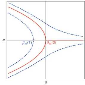
β
h
βzz0
βzzT
FIG. 2. (Color online) Bifurcation diagram (order parameter h as a function of the bifurcation parameter β) of the noisy zigzag bifurcation, after Ref. [43]. The solid red line is the diagram of a supercritical pitchfork bifurcation without noise, and βzz(0) is the deterministic threshold. The blue dashed line indicates the blurring of the bifurcation, because of the zone of local fluctuations that surround the equilibrium state. βzz(T ) is the thermal threshold, and βzz(T )!
β! βzz(0) defines the bifurcation region in the bifurcation parameter
space.
Although this longitudinal confining potential determines the equilibrium positions of the particles [11,49], it has no other direct influence on the transverse fluctuations. The previous calculation of the deterministic threshold becomes cumbersome in this case, because the particles cease to be equivalent [10,11,19–23,26–28,31], so that both x∗
n− xn∗−1=
dnand the absolute value of the transverse displacement hn
depend on the particle rank n. It is thus much simpler to get the deterministic bifurcation threshold from the vibration modes [24,32–35,38,50], as explained in the Appendix and shown in the inset of Fig.7(b).
In this paper we focus on a strong subdiffusive behavior for the transverse thermal fluctuations of the particles close to the zigzag transition (see Sec.IIIbelow). At finite (nonzero) temperature, the actual definition of the threshold for the zigzag bifurcation is not obvious, because the thermal fluctuations transform the supercritical bifurcation into a smooth transition [42–47]. The theory predicts that the diagram of a noisy bifurcation is blurred with respect to that of a purely me-chanical bifurcation and the existence of abifurcation region
in which flips between equivalent zigzag configurations occur [43,45,47]. Those flips become forbidden below a thermal bifurcation threshold βzz(T ), which is shifted with respect
to the deterministic threshold βzz(0) ≡ βzz [43,47]. This is
illustrated in Fig.2.
III. SIMULATION RESULTS A. Simulations protocol
In the simulations, the summation of Eq.(1) is extended to all m ̸= n. In most experimental situations [10,26–28] Uint(r) is a repulsive potential. We use a screened electrostatic
DELFAU, COSTE, AND SAINT JEAN PHYSICAL REVIEW E87, 032163 (2013) 0.01 0.1 1 10 100 0.1 0.2 0.5 1.0 2.0 5.0 10.0 Time s y 2 µ m 2 a 0.01 0.1 1 10 100 0.1 0.2 0.5 1.0 2.0 5.0 10.0 Time s y 2 µ m 2 b
FIG. 4. (Color online) Plot of the transverse MSD (µm2) as a function of time (s), in logarithmic scales, for 30 particles with periodic boundary conditions, γ = 10 s−1 and T = 107 K. We compare simulations data above [red (dark grey) dots, ϵ > 0] and below [green (light grey) dots, ϵ < 0] the zigzag transition. (a) |ϵ| = 1.7 × 10⁻⁴; (b) |ϵ| = 9.5 × 10⁻⁴. In each plot, the thin solid black line shows the asymptotic behavior in the thermodynamic limit, Eq.(12).
realize this regime, strong correlations between the particles’ motions are necessary. Here, in contrast with the case of lon-gitudinal fluctuations, the ordering of the particles cannot be invoked to explain these correlations. In the case of transverse fluctuations, the correlations only appear in the vicinity of the transition β → βzz, because of the zigzag pattern that induces
a soft mode which dominates the dynamics.
The transverse SFD behavior is observed on both sides of the zigzag transition, as shown in Fig.4for two small values of |ϵ|, a low temperature T = 107 K, and γ = 10 s−1. The
data sets for which ϵ > 0 are almost indistinguishable from those for which ϵ < 0. This is consistent with the peculiarities of a supercritical pitchfork bifurcation. As will be shown in Sec.IV, the SFD regime is linked to the soft mode that takes place on both sides of the transition, and corresponds to the critical slowing down of the dynamics [41]. Moreover, the bifurcation is continuous, hence the amplitude of the zigzag equilibrium for ϵ < 0 scales as √|ϵ|. Thus very near the bifurcation threshold, the transverse confining force and the repulsive interactions result in an effective transverse stiffness βzzϵ. The transverse fluctuations are therefore those of a
particle in a potential well of stiffness ∼βzz|ϵ| on both sides of
the transition. This explains why the transverse fluctuations have the same magnitude. At large time they eventually saturate at a value that scales as 1/√ϵ. This is actually the case for the data displayed in Fig.3. In this figure, we also compare the transverse SFD regime with that for an infinite system in the thermodynamic limit, given in Eq.(12). We see that despite the rather small number of particles (N = 30) the agreement is excellent. The complete solution of Eq. (9), which is valid for a finite number of particles, is shown in Figs.3(b)and3(d). There is no free parameter in the analysis, and the agreement between the calculations and the simulation data is almost perfect.
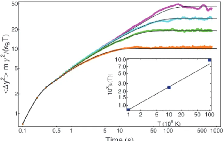
Let us now discuss some finite temperature effects. A more complete analysis will be published later [48]. To this aim, we study the time evolution of the dimensionless transverse MSD ⟨ #!y2⟩ ≡ Mγ2⟨!y2⟩/(kBT) that is independent on the
temperature T according to Eq.(9). In Fig.5, we plot it for 107! T ! 1010K, hence a dimensionless interaction energy
105! U
int(d)/(kBT)! 102. The data clearly show that ⟨ #!y2⟩
actually depends on the temperature.
This may be interpreted in the light of noisy bifurcation theory. As shown by Agez et al. [47], at finite temperature an intrinsic bifurcation point ϵ(T ) occurs, which is shifted
from the deterministic bifurcation point ϵ = 0, with in our specific case ϵ(T ) < 0 and |ϵ(T )| an increasing function of the temperature (see Fig. 2 for an illustration of this idea). The dimensionless transverse MSD ⟨ #!y2⟩ depends upon ϵ through the frequency spectrum (q defined in Eq.(10)that
may be written (2q k = βzz M $ ϵ+ cos2qk 2 % . (5)
If this picture is correct, at temperature T the actual dimen-sionless distance toward the zigzag threshold is ϵ − ϵ(T ). We thus inject a fitting parameter ϵfitin Eq.(9), which provides a
0.1 0.5 1 5 10 50 100 500 1000 1 2 5 10 20 50 Time s y 2 m γ 2 kB T 1 2 5 10 20 50 100 1.0 10.0 5.0 2.0 3.0 1.5 7.0 T 108K 10 3 T∋
FIG. 5. (Color online) Plot of the dimensionless transverse MSD, Mγ2⟨!y2⟩/(kBT), as a function of time (s), in logarithmic scales, for 30 particles and periodic boundary conditions. In the simulations γ = 10 s−1, ϵ = 0.0010 and from top to bottom plots T = 107 K (magenta), T = 108 K (cyan), T = 109 K (green), T = 1010 K (orange). Without the thermal noise effect on the bifurcation, all data should be on the same curve. The solid black lines correspond to the calculation in Eq.(9), with ϵfitequal to, from top to bottom plot, 0.0010 (magenta), 0.0018 (cyan), 0.0035 (green), and 0.0105 (orange). In the inset, we plot 103|ϵ(T )| as a function of 108T, in logarithmic scale. The solid line is of slope 1/2.
TRANSVERSE SINGLE-FILE DIFFUSION NEAR THE . . . PHYSICAL REVIEW E87, 032163 (2013) measurement of ϵ(T ) = ϵ − ϵfit. At low temperature ϵ(T ) = 0,
which is consistent with the data analysis shown in Figs.3and
4for which ϵfit= ϵ. The striking feature exhibited by Fig.5is
that the single fitting parameter ϵfitis sufficient to fully describe
the entire time evolution of ⟨ #!y2⟩ at large temperature. In the inset of Fig.5we plot the values of ϵ(T ) deduced from ϵfitas
a function of the temperature T , and see that it is consistent with the√T scaling predicted by Agezet al. [47].
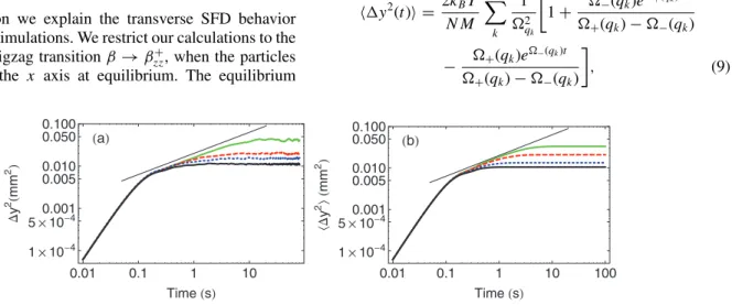
C. Transverse SFD in finite boxes
In quasi-1D systems of finite size, the particles are not equidistant at equilibrium, and in the zigzag pattern the distance of a particle from the longitudinal axis depends upon its rank in the chain. However, the configurational transition is as before a supercritical pitchfork bifurcation occurring at a critical value of the transverse confining potential [22,27,
28,31,51]. As for periodic boundary conditions, the particle’s transverse fluctuations are thus strongly correlated near the transition. Since interparticle distances are the smallest in the cell center [10,11], the SFD behavior for transverse motions is most easily observed for the center particles. A convincing example is provided by Fig.6(a), where the MSD of the center particle exhibits the typical SFD behavior near the zigzag transition, at ϵ = 0.01.
In Fig.6(b), we display the analytical results given in the Appendix [see Eq.(A2)], which are in very good agreement with the simulations. We also display the scaling law in the thermodynamic limit given by Eq. (12), in which we replace βzz by the value βzz(N,λw) for the corresponding
finite box [see inset of Fig.7(b)]. We see that the agreement is very good although the particle’s number is not very large (N = 33), and although the confining potential is not of very short range (L/λw= 7.5; for a precise classification of the
confining potentials see Ref. [49]).
IV. THEORETICAL DESCRIPTION OF THE TRANSVERSE SFD
In this section we explain the transverse SFD behavior observed in the simulations. We restrict our calculations to the vicinity of the zigzag transition β → β+
zz, when the particles
are aligned on the x axis at equilibrium. The equilibrium
positions of the particles are thus r∗
n= (xn∗,0). In the most
general case, dn≡ xn∗− x∗n−1 depends on the particle rank n.
Let
|rn− rn−1| = [(dn+ un− un−1)2+ (yn− yn−1)2]1/2, (6)
where yn and un are respectively the small fluctuations in
the transverse and longitudinal directions. The dynamics of the thermal fluctuations around the equilibrium positions is easily deduced from Eq. (1) where for simplicity we restrict the analysis to nearest neighbors’ interactions, m = n+ 1. Expanding Eq. (1) up to second order in the small quantities un/dn and yn/dn, we may calculate the transverse
and longitudinal forces exerted on the particle n, −∂E/∂yn,
and −∂E/∂un. The longitudinal and transverse fluctuations
are uncoupled, and the Langevin equation for the transverse fluctuations reads ¨yn+ γ ˙yn+ 1 M[(β − βn+1− βn)yn+ βn+1yn+1+ βnyn−1] = µ(n,t) M , (7)
where for simplicity we drop the index in µy(n,t), and with
βn≡ −Uint′ (dn)/dn. Formally, this equation is very similar to
the one for longitudinal fluctuations [5,11].
We hereafter restrict the calculations to the case of periodic boundary conditions, and treat the case of the finite boxes in the Appendix. Therefore, x∗
n = nd with d the mean interparticle
distance and all βn= β = −Uint′ (d)/d. As in [5], we perform
a discrete Fourier transform Y(qk,t) = N ! l=1 eiqkly l(t), yl(t) = 1 N N ! k=1 e−iqklY(q k,t), (8)
where qk= −π + 2πk/N for k= 1, . . . ,N ensures
yN+l(t) = yl(t). It is easily seen that each mode Y (qk,t)
behaves as a particle of mass M in a harmonic potential well, and that the MSD in the transverse direction is [5]
⟨!y2(t)⟩ = 2kBT N M ! k 1 (2q k & 1 + (−(qk)e(+(qk)t (+(qk) − (−(qk) − (+(qk)e (−(qk)t (+(qk) − (−(qk) ' , (9) 0.01 0.1 1 10 1 104 5 100.0014 0.005 0.010 0.050 0.100 Time s y 2 mm 2 a 0.01 0.1 1 10 100 1 104 5 100.0014 0.005 0.010 0.050 0.100 Time s y 2 mm 2 b
FIG. 6. (Color online) Plot of the transverse MSD (mm2) for the center particle, as a function of time (s), in logarithmic scale, for 33 particles and fixed boundary conditions. The range of the longitudinal confinement is λw= 4 mm, Ew= 0.1E0, T = 109K, and γ = 10 s−1. In both plots the black solid line is the behavior in the thermodynamic limit, Eq.(12), with βzzreplaced by its critical value βzz(N,λw) for the simulated finite box. (a) Simulations, for ϵ = 0.010 (green, light grey), ϵ = 0.019 (dashed red line), ϵ = 0.038 (dotted blue line), and ϵ = 0.058 (solid black line). (b) Analytical calculations, from Eq.(A2)with the same color code.
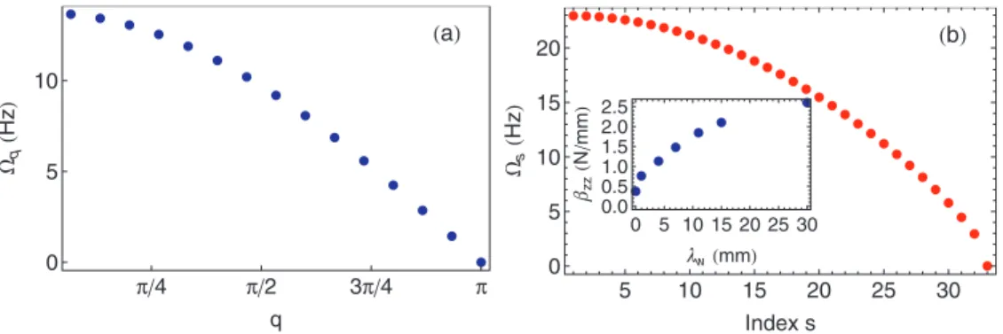
DELFAU, COSTE, AND SAINT JEAN PHYSICAL REVIEW E87, 032163 (2013) π 4 π 2 3π 4 π 0 5 10 q q Hz a 5 10 15 20 25 30 0 5 10 15 20 Index s s Hz b 0 5 10 15 20 25 30 0.0 0.5 1.0 1.5 2.0 2.5 λw mm βzz N mm
FIG. 7. (Color online) (a) Plot of the frequency spectrum (q(Hz) as a function of the dimensionless wave number q for periodic boundary conditions, for 30 particles, for a period of 60 mm and β = βzz. The modes for negative q are symmetric with respect to the q = 0 axis. (b) Plot of the frequencies (s(Hz) as a function of the mode index s for 33 particles, for a cell of length 60 mm, for λw= 4 mm and β = βzz(λw). Inset: Plot of βzz(N,λw) (N/mm) as a function of λw(mm), for Ew= 0.1E0and N = 33. The abscissa λw= 0 corresponds to periodic boundary conditions. with (±(qk) ≡ − γ 2 ± " γ2 4 −(2qk, (10) (2qk ≡ 1 M $ β− 4β sin2 qk 2 % .
A plot of (qk is shown in Fig. 7(a) for β = 4β. At this
particular value, a soft mode (±π = 0 appears. The shape of this mode is an alternate transverse displacement of the particles, and the vanishing of its frequency indicates the zigzag transition. We thus recover our previous result for βzz,
Eq.(2)
The physical origin of the soft mode is clear: exactly at the transition, there is no restoring force for the mode q±N = ±π. The calculation of the characteristic frequencies is a classic way to determinate the zigzag threshold from the vanishing of one frequency [24,32–35,38,50]. This method is particularly efficient for finite boxes, for which the critical value βzzmust
be determined numerically. A frequency spectrum is shown in Fig.7(b)for the particular value βzz(N,λw) at which a soft
mode of zero frequency appears. A plot of βzz(N,λw) as a
function of the confinement range λwis shown in the inset of
Fig.7(b). The zigzag transition is favored by the confinement because the distance between the inner particles decreases, so that moving away from the x axis becomes energetically favorable at higher values of β. This explains the increase of βzz(N,λw) with the confinement length λw.
A. Transverse SFD in the thermodynamic limit The long time behavior of the MSD may be computed in closed form from Eq.(9)near the zigzag transition β → 4β|+,
in the thermodynamic limit N → ∞. Replacing the discrete sums by integrals, with the rule (1/N)(k−→ (1/2π))π
−π, we may write ∂⟨!y2(t)⟩ ∂t = 2kBT m 1 π * π 0 dq e(+(q)t− e(−(q)t (+(q) − (−(q), (11) where we have used the invariance q → −q. The large time asymptotic behavior of this integral may then be determined by the Laplace method [52]. For t → ∞, the integral is dominated
by the immediate neighborhood of the point corresponding to the maximum value of either (+(q) or (−(q) in [0,π]. From Eq.(10), we see that a maximum of (+(q) takes place at q = π, with (+(π) = 0, (′+(π) = 0, and (′′+(π) < 0. A
simple calculation then gives ⟨!y2(t)⟩t→∞∼ √4kBT
π Mγ βzz
t1/2. (12) This establishes that the transverse fluctuations of an infinite system, in the thermodynamic limit, undergo the typical SFD behavior with a t1/2scaling.
For longitudinal as well as transverse fluctuations, the SFD behavior is strongly linked to the existence of a finite band of overdamped modes. Those low frequency modes are in the vicinity of a peculiar mode, the frequency of which vanishes. For longitudinal fluctuations, the mode of vanishing frequency is the one with null wave number associated to translational invariance [5]. For transverse fluctuations, the mode of vanishing frequency is the soft mode of wave number ±π associated to the zigzag transition.
B. Transverse SFD in finite periodic systems
At very short time, all N terms in the sum(9)are equal so that ⟨!y2(t)⟩t→0
∼ (kBT /M)t2. We recover the obvious result
that, at very short time, all particles are uncorrelated and undergo a ballistic motion at temperature T . The prefactor is, of course, the same as for longitudinal fluctuations [5] since the very short time motions are isotropic.
Let us now consider the intermediate regime, before the saturation, assuming that we are exactly at the zigzag transition β = 4β. Using a linear approximation of the dispersion relation for qk→ π, as done in [5] for longitudinal fluctuations
(hence qk→ 0), with the help of the Debye approximation,
we get (2 qk ∼ βδ
2
k/Mwhere δk≡ π − qk. Let us also assume
a large damping, γ ≫ 2(0. Thus (−(qk) ∼ −γ , (+(qk) ∼
−(2qk/γand (+(qk) − (−(qk) ∼ γ . In the sum(9), each mode
(qk eventually saturates at the time t ∼ γ /(
2
qk. Hence, at a
given time t, the modes which are not saturated have a wave number such that (2
qk < γ /tor δk <(
Mγ βt)
1/2. There are n(t)
modes which are not saturated, with n(t) ∼ 2N 2π(
Mγ βt )
1/2 (the
TRANSVERSE SINGLE-FILE DIFFUSION NEAR THE . . . PHYSICAL REVIEW E87, 032163 (2013) factor 2 takes into account the symmetry qk←→ −qk). In the
sum(9)we drop the subdominant terms e(−(qk)tto obtain
⟨!y2(t)⟩ ∼ 2kBT N M ! k 1 (2qk ⎡ ⎣1 − γ -1 −(2qkt γ . γ ⎤ ⎦ ∼ N Mγ2kBT $ ! k % 1 23 4 =n(t) t∼ 2 πkBT $ t Mγ β %1/2 . (13)
This rough estimate for intermediate times establishes the existence of a SFD regime for transverse fluctuations in finite periodic systems, and a comparison with the exact formula given in Eq.(12)shows that the approximate prefactor is quite close to the exact one.
The dependence of the saturation value of the transverse MSD on the transverse stiffness may also be estimated as follows. Let us assume that we are near the zigzag transition, that is, β = 4β(1 + ϵ) with 0 < ϵ ≪ 1. Both (±(qk) are
strictly negatives, so that at large time each term in the sum(9) saturates toward 1/(2
qk. The sum is thus dominated
by the small frequency modes, with a wave number such that δk= π − qk≪ 1. Their frequency is (2qk ≈ β(4ϵ + δ
2 k)/M,
which stays small up to δk ∼ 2√ϵ. The index k associated to
the last mode is k ∼ Nδk/(2π) ∼ N√ϵ/π. The MSD at long
time may thus be approximated as ⟨!y2(t)⟩t→∞∼ 22kN MBT N √ϵ π M 4βϵ ∼ kBT π βϵ1/2. (14) This estimate is in good agreement with the simulations data displayed in Fig.3.
From the results (13) and (14) it is easy to get an expression for the time tsat taken by the system to reach the
saturation when the zigzag transition is approached. Assum-ing [tsat/(Mγ β)]1/2∼ kBT /(πβϵ1/2), we get tsat∼ Mγ /(βϵ).
The saturation time diverges at the transition ϵ → 0, and the scaling law tsat∝ ϵ−1exhibits the critical slowing down in the
vicinity of a supercritical pitchfork bifurcation [41].
V. CONCLUSION
In this paper we have studied the transverse fluctuations in quasi-1D systems of particles in a thermal bath, near the zigzag transition. We have demonstrated that close to the zigzag threshold, the transverse fluctuations exhibit the typical SFD behavior, with a MSD that scales as the square root of time. This subdiffusive behavior traces back to strong interparticle correlations, and is observed on both sides of the transition. In contrast with the longitudinal fluctuations, for which the correlations are due to the noncrossing condition, the transverse motions of the particles are only correlated close to the zigzag transition. Their dynamics is closely linked to the overdamped modes in the vicinity of the soft mode that appears at the transition, and replaces the zero frequency mode due to translational invariance for longitudinal motion [5,15].
The small thermal fluctuations may be described by the lin-earization of the full dynamical equations in the neighborhood of the equilibrium positions, close to the zigzag transition, when the equilibrium positions are still aligned. In this
configuration, longitudinal and transverse motions are decou-pled in the linear regime, so that an adaptation of our previous calculations [5,11] is obvious. We have calculated analytically the MSD ⟨!y2(t)⟩ and found an excellent agreement with the
simulations data. In the thermodynamic limit we demonstrate the existence of the SFD regime at the zigzag transition. We calculate the mobility for transverse fluctuations and find a perfect agreement with the simulations. For finite sized systems, we are able to recover this result up to a numerical factor.
The zigzag transition is a supercritical pitchfork bifurcation, whose features depend on the thermal noise in the system. At high temperature, the MSD is still quite well described by our model, if only we take into account a shift in the bifurcation threshold that increase with the thermal noise level, hence with the temperature. We find a good agreement between this shift and the predictions of stochastic bifurcation theory [47]. In a future work [48], we will show that the measurement of the duration of the SFD regime provides a very efficient way to determine the bifurcation threshold in a system which undergoes thermal noise.
APPENDIX: FINITE BOXES
We consider a system of 2N − 1 moving particles xi with
i= −N + 1, . . . ,N − 1. Since the longitudinal confining potential depends only on x, the transverse motion of particles ±(N − 1) is free in contrast with Ref. [11]. We distinguish the long-ranged longitudinal confining potentials, the influence of which extends toward the inner particles of the cell, from the short-ranged potentials for which all particles are equidistant with a distance d, except the outermost ones which are at a distance dw from the fixed walls [49]. In this latter case,
Eq.(7)is that of a chain of identical masses and springs with free boundary conditions. The relevant frequencies may be calculated analytically [53], (2s ≡ 1 M & β+ 4U ′ int(d) d cos 2 (2N − s)π 2(2N − 1) ' , (A1)
with s = 1, . . . ,2N − 1. The maximum frequency corre-sponds to s = 1, when all particles oscillate in phase in the confining transverse potential. The zigzag transition happens when a frequency vanishes, for s = 2N − 1 hence βzz= −4[Uint′ (d)/d] cos2{π/[2(2N − 1)]}. The result(10)is
recovered in the limit N → ∞, as expected since in the thermodynamic limit both systems are identical.
In the general case of long-ranged longitudinal confining potentials, the eigenfrequencies (sand the orthogonal
eigen-modes Ys(n) of unit norm are calculated numerically for the
Hessian matrix deduced from Eq. (7). It is a simple task to show that Eq.(9)is replaced by [11]
⟨!y2(n,t)⟩ = 2kMBT 2N−1! s=1 Ys(n)2 (2s & 1 + ( s −e( s +t (s+− (s− − (s +e( s −t (s+− (s− ' , (A2)
DELFAU, COSTE, AND SAINT JEAN PHYSICAL REVIEW E87, 032163 (2013) where (s±≡ −γ 2 ± " γ2 4 −(2s. (A3)
Once the normal frequencies and the components of the normal modes are known, the dynamics of the transverse
fluctuations is completely determined by Eq. (A2). The calculations are displayed in front of the simulations in Fig. 6(b), showing a very good agreement, without any free parameter since the relevant Hessian matrix is fully determined once the equilibrium positions are known from the simulations [11].
[1] A. Hodgkin and R. Keynes, J. Physiol.128, 61 (1955). [2] D. Jepsen,J. Math. Phys.6, 405 (1965).
[3] M. Kollmann,Phys. Rev. Lett.90, 180602 (2003).
[4] B. Felderhof,J. Chem. Phys.131, 064504 (2009).
[5] J.-B. Delfau, C. Coste, and M. Saint Jean, Phys. Rev. E84,
011101 (2011).
[6] T. Ooshida, S. Goto, T. Matsumoto, A. Nakahara, and M. Otsuki, J. Phys. Soc. Jpn.80, 074007 (2011).
[7] H. van Beijeren, K. W. Kehr, and R. Kutner,Phys. Rev. B28,
5711 (1983).
[8] L. Lizana and T. Ambj¨ornsson,Phys. Rev. Lett.100, 200601
(2008).
[9] L. Lizana and T. Ambj¨ornsson,Phys. Rev. E80, 051103 (2009).
[10] J.-B. D. Delfau, C. Coste, C. Even, and M. Saint Jean,Phys. Rev. E82, 031201 (2010).
[11] J.-B. Delfau, C. Coste, and M. Saint Jean,Phys. Rev. E85,
061111 (2012).
[12] Q.-H. Wei, C. Bechinger, and P. Leiderer,Science 287, 625
(2000).
[13] C. Lutz, M. Kollmann, and C. Bechinger,Phys. Rev. Lett.93,
026001 (2004).
[14] B. Lin, M. Meron, B. Cui, S. A. Rice, and H. Diamant,Phys. Rev. Lett.94, 216001 (2005).
[15] C. Coste, J.-B. Delfau, C. Even, and M. Saint Jean,Phys. Rev. E81, 051201 (2010).
[16] K. Nelissen, V. Misko, and F. Peeters,Europhys. Lett.80, 56004
(2007).
[17] S. Herrera-Velarde and R. Casta˜neda-Priego,J. Phys.: Condens. Matter19, 226215 (2007).
[18] S. Herrera-Velarde and R. Casta˜neda-Priego,Phys. Rev. E77,
041407 (2008).
[19] M. G. Raizen, J. M. Gilligan, J. C. Bergquist, W. M. Itano, and D. J. Wineland,Phys. Rev. A45, 6493 (1992).
[20] I. Waki, S. Kassner, G. Birkl, and H. Walther,Phys. Rev. Lett.
68, 2007 (1992).
[21] J. P. Schiffer,Phys. Rev. Lett.70, 818 (1993).
[22] S. Seidelin, J. Chiaverini, R. Reichle, J. J. Bollinger, D. Leibfried, J. Britton, J. H. Wesenberg, R. B. Blakestad, R. J. Epstein, D. B. Hume, W. M. Itano, J. D. Jost, C. Langer, R. Ozeri, N. Shiga, and D. J. Wineland,Phys. Rev. Lett.96,
253003 (2006).
[23] R. Blatt and D. Wineland,Nature (London)453, 1008 (2008).
[24] J. P. Home, D. Hanneke, J. D. Jost, D. Leibfried, and D. J. Wineland,New J. Phys.13, 073026 (2011).
[25] M. Mielenz, H. Landa, J. Brox, S. Kahra, G. Leschhorn, M. Albert, B. Reznik, and T. Schaetz, arXiv:1211.6867[Phys. Rev. Lett. (to be published)].
[26] B. Liu and J. Goree,Phys. Rev. E71, 046410 (2005).
[27] A. Melzer,Phys. Rev. E73, 056404 (2006).
[28] T. E. Sheridan and K. D. Wells, Phys. Rev. E 81, 016404
(2010).
[29] T. E. Sheridan and A. Magyar,Phys. Plasmas17, 113703 (2010).
[30] D. H. E. Dubin,Phys. Rev. Lett.71, 2753 (1993).
[31] D. H. E. Dubin,Phys. Rev. E55, 4017 (1997).
[32] G. Morigi and S. Fishman,Phys. Rev. Lett.93, 170602 (2004).
[33] G. Morigi and S. Fishman,Phys. Rev. E70, 066141 (2004).
[34] S. Fishman, G. De Chiara, T. Calarco, and G. Morigi,Phys. Rev. B77, 064111 (2008).
[35] G. Astrakharchik, G. De Chiara, G. Morigi, and J. Boronat, J. Phys. B42, 154026 (2009).
[36] T. Sheridan,Phys. Scr.80, 065502 (2009).
[37] G. De Chiara, A. del Campo, G. Morigi, M. Plenio, and A. Retzker,New J. Phys.12, 115003 (2010).
[38] J. E. Galv´an-Moya and F. M. Peeters,Phys. Rev. B84, 134106
(2011).
[39] E. Shimshoni, G. Morigi, and S. Fishman,Phys. Rev. Lett.106,
010401 (2011).
[40] J. Guckenheimer and P. Holmes, Nonlinear Oscillations, Dynamical Systems, and Bifurcations of Vector Fields (Springer-Verlag, New York, 1983).
[41] P. Manneville, Dissipative Structure and Weak Turbulence (Academic, New York, 1990).
[42] P. Hanggi, T. J. Mroczkowski, F. Moss, and P. V. E. McClintock, Phys. Rev. A32, 695 (1985).
[43] C. Meunier and A. Verga,J. Stat. Phys.50, 345 (1988).
[44] J. B. Swift, P. C. Hohenberg, and G. Ahlers,Phys. Rev. A43,
6572 (1991).
[45] N. van Kampen,Stochastic Processes in Physics and Chemistry (North-Holland, Amsterdam, 1992).
[46] P. C. Hohenberg and J. B. Swift,Phys. Rev. A46, 4773 (1992).
[47] G. Agez, M. G. Clerc, and E. Louvergneaux,Phys. Rev. E77,
026218 (2008).
[48] J.-B. Delfau, C. Coste, and M. Saint Jean (unpublished). [49] J.-B. Delfau, C. Coste, and M. Saint Jean, Phys. Rev. E85,
041137 (2012).
[50] D. H. E. Dubin and J. P. Schiffer, Phys. Rev. E 53, 5249
(1996).
[51] D. Lucena, D. V. Tkachenko, K. Nelissen, V. R. Misko, W. P. Ferreira, G. A. Farias, and F. M. Peeters,Phys. Rev. E85, 031147
(2012).
[52] A. Nayfeh,Introduction to Perturbation Techniques (Wiley, New York, 1993).
[53] L. Brillouin and M. Parodi, Propagation des Ondes dans les Milieux P´eriodiques (Masson, Paris, 1956).