Data monitoring web services in a virtual lab environment

(1)

Data Monitoring Web Services in a Virtual Lab Environment

By

Ashish Sadashiv Kulkarni

B.Tech. Chemical Engineering, IIT Madras, 1999

M.S. Chemical Engineering, PennState University, 2001

Submitted to the Department of Civil and Environmental Engineering in

partial fulfillment of the requirements for the Degree of

MASTER OF ENGINEERING IN

CIVIL AND ENVIRONMENTAL ENGINEERING

AT THE

MASSACHUSSETS INSTITUTE OF TECHNOLOGY

JUNE 2002

@ 2002 Ashish Sadashiv Kulkarni. All rights reserved

The author hereby grants to MIT permission to reproduce and to distribute publicly

paper and electronic copies of this thesis document in whole or in part.

A uthor...

...

Ashish Sadashiv Kulkarni

Department of Civil and Environmental Engineering

May 13, 2001

Certified.

.. . . . ... : . ... Kevin Amaratunga Assistant Professor, Department of Civil and Environmental Engineering

Accepted by... ...

Oral Buyukozturk Chairman, Departmental Committee in Graduate Studies

MASSACHUSETTS INSTITUTE OF TECHNOLOGY

(2)

(3)

Data Monitoring Web Services in a Virtual Lab Environment

By

Ashish Sadashiv Kulkarni

Submitted to the Department of Civil and Environmental Engineering on May 24, 2002 in partial fulfillment of the requirements for the Degree of

Master of Engineering in Civil and Environmental Engineering

ABSTRACT

Environmental issues have become of prime concern due to dramatic increase in the pollution levels in all parts of the world. Underlying aquifer flow in environmentally sensitive places plays an important role in characterizing the environmental condition of the place. There is thus a pressing need for monitoring and real time analysis of hydrological data over areas of environmental interest. Coupling the emerging sensing and wireless technologies with an internet infrastructure can enable efficient data monitoring and real-time analysis of environmental conditions over an area of interest. Information gathered from various data sources regarding the change in water level and quality during various seasons can then be used to characterize trends in the physical, chemical and biological condition of the environment.

Efficient real-time monitoring furnished with fast data rendering and decision-making capabilities can go a long way in monitoring Civil and Environmental Engineering infrastructure. The speed and reliability necessary for such a task can be achieved only by using a distributed infrastructure, with dedicated resources to data acquisition, archival and rendering. Distributed development technologies like DCOM, CORBA, RMI and SOAP, essentially extensions of simple RPC protocols, provide the interconnectivity between different components of such a distributed infrastructure. The present work discusses these distributed development technologies and compares them in the context of the Smartwells project.

Thesis Supervisor: Dr. Kevin Amaratunga

(4)

(5)

ACKNOWLEDGEMENTS

I would like to dedicate this thesis to my family who provided the inspiration and

encouragement for me to come to M.I.T.

I would like to thank my thesis advisor Dr. Kevin Amaratunga for his tutelage and

assistance throughout this learning process. I would also like to thank Dr. Eric Adams, my advisor for the Smartwells project for his help and guidance during the project. Also, I would like to express special gratitude to fellow M.S. student Ragunathan Sudarshan, for his help and support throughout the course of the project.

I am also very thankful to Raghu Narayan, fellow partner in the Smartwells Project for

the constant support during my year at MIT.

Finally, I would like to thank God for blessing me with the opportunity to pursue my education this far.

(6)

(7)

List of Tables

2.1 Specifications for water level sensor WL300... 22

2.2 Specifications for conductivity level sensor ... 24

2.3 Specifications for Rain Gauge RG600... 26

2.4 Specifications for FP-AI-110 1/0 Module ... 28

2.5 Sampling Rates for FP-AI-110... 29

2.6 Specifications for FP-1600 Network Module ... 30

2.7 Transfer Rates for FP-1000 [with FP-AI-110 1/0 module]... 31

2.8 Services running on the Smartwells server ... 35

(12)

CHAPTER 1

INTRODUCTION

The purpose of this thesis is to examine the use of different distributed development technologies and their application in the context of a real-time data monitoring project. The project in consideration is 'Smartwells' -a student initiative in the Department of Civil and Environmental Engineering at the Massachusetts Institute of Technology (MIT), Cambridge, Massachusetts. The 'Smartwells' project, sponsored by the MIT-Microsoft i-Campus Alliance, started in May 2001 and presently consists of three Master's students and two faculty advisors, Prof. Kevin Amaratunga and Dr. Eric Adams.

The 'Smartwells' Project introduces the virtual laboratory concept (also known as I-Labs) to environmental engineering education at MIT. The objective of the project is to develop a network of permanently instrumented boreholes -the 'smart wells', which continuously monitor groundwater conditions over an area of hydrological interest. When coupled with sensors for monitoring external influences such as precipitation and contaminant sources, the 'Smartwells' network provides a rich educational infrastructure. 'Smartwells' combines the benefits of traditional indoor laboratories and field excursions. In addition to real-time data monitoring, this project is also intended as an educational visualization tool for the undergraduate courses offered

by the Department of Civil and Environmental Engineering. Students have online access to

hydrological data in a quasi-laboratory setting and at the same time have the opportunity to study the complexities of a real-world hydrological system.

1.1 Motivation

In the information age, environmental issues have become of prime concern due to dramatic increase in the pollution levels in all parts of the world. Underlying aquifer flow in environmentally sensitive places plays an important role in characterizing the environmental condition of the place. Ground water flow in such places of hydrologic interest has to be

(13)

monitored in order to characterize the groundwater and identify changes or trends in water quality over time. This could help in identifying existing or emerging water quality problems. Information gathered from various data sources regarding the change in water level and quality during various seasons can be used to characterize trends in the physical, chemical and biological condition of the environment. There is thus a pressing need for environmental data monitoring in places of hydrological and environmental interest. Real time analysis of such acquired data will help us address many environmental challenges faced by the industry. Information technology enables us to integrate two systems for continuous data acquisition and analysis and accomplish the task of real-time data monitoring and control. Coupling the emerging sensing technology with an Internet infrastructure can enable efficient data monitoring of conditions over an area of interest.

With the rapid proliferation of networked devices, accelerated by the growth of Internet and wireless communication standards, the next generation in monitoring systems seems to be that of wireless sensor networks. Such advances in sensing technology find very useful applications in Civil Engineering systems. In a sensor rich environment, it is essential to process large chunks of data efficiently and reliably to be able to come to reasonable conclusions about the state of the system. Efficient real-time monitoring coupled with fast data rendering and decision-making capabilities can go a long way in monitoring Civil and Environmental Engineering infrastructure.

1.2 Purpose

The 'Smart Wells' project aims at real-time hydrologic and water table monitoring of wells from a remote location using a combination of wireless sensor network, state-of-the-art sensors for measurement, data acquisition and visual rendering of acquired data on a mobile computer. We are developing a website which allows real-time access to acquired hydrologic data providing a perpetual monitoring capability, the ability to analyze acquired data with visual rendering tools, and a data archiving capability for later studies. This project will be used by students/professors from Hydrology and Environmental Engineering to study groundwater

(14)

hydrology in their classrooms and laboratories. The results and source code will be available in the public domain for use by other academic institutions. The project can be deployed in actual

field settings with a proper scale-up of the wireless sensor network.

1.3 Layout of the thesis

Chapter 2 discusses the Smartwells project giving an overview of the same. This is followed by the software-hardware interface aspect of data collection, discussing how to interface the measuring equipment with the monitoring server through the Internet. The development environment is described followed by the internals of data-polling from the instrument. The chapter also discusses the sensors used and interfacing the data acquisition hardware to a computer. This is followed by details on how to broadcast data using TCP/IP sockets using the multithreaded DataSocket API available from National Instruments. The later sections deal with archiving real-time data in a database. The database model is discussed along with the JDBC classes used to communicate with back-end SQL based databases. Finally, the processing and visualization of live and archived data is discussed. The client side code for retrieving data from a DataSocket server and techniques to retrieve data from a database are reviewed. Chapter 3 focuses on different distributed development technologies such as DCOM, CORBA and Java/RMI. A distributed application sample is discussed in the context of the Smartwells project. Later, these technologies are compared and their drawbacks are discussed. Emerging technologies such as SOAP are introduced and their advantages on the older technologies are cited. Chapter 4 then deals with the architecture and design of the newer distributed technologies, specifically SOAP. An application sample in the context of Smartwells is again discussed. Chapter 5 then concludes the material presented in the thesis, and details further goals of the work. The appendices have additional details pertaining to the implementation of the software. Appendix A covers the IDL interface, client and server side code for the application sample implemented using DCOM, CORBA and Java/RMI.

(15)

CHAPTER 2

SMARTWELLS PROJECT

This chapter starts with an overview of the Smartwells project. It then addresses the remote-monitoring hardware aspects of the project [8, 9, 17-19, 21]. The primary focus is on the sensors used for monitoring aquifers such as the Smartwells. The section on data acquisition systems focuses on the distributed system, FieldPoint, manufactured by National Instruments, and the interface between the measuring equipment and the server monitoring via the Internet. The chapter also discusses the issue of interfacing the data acquisition hardware to a computer. The development environment is described, followed by internals of data-polling from the instrument. This is followed by details on how to broadcast data using TCP/IP sockets using the multithreaded DataSocket API available from National Instruments. The later sections deal with archiving real-time data in a database. The database model is discussed along with the JDBC classes used to communicate with back-end SQL based databases. Finally, the processing and visualization of live and archived data is discussed. The client side code for retrieving data from

a DataSocket server and techniques to retrieve data from a database are reviewed.

2.1 Pro* ect Overview

The main objective of the Smartwells project was to design and implement a scaleable, real-time system to monitor aquifer hydrology. This would cover the sensing, transmission, archival and rendering aspects of the whole system. The goal was also to experiment with the state of the art in sensing and monitoring, including different hydrological sensors and emerging wireless standards like IEEE 802.11. Then, data obtained by the system was to be made available in real-time as well as in archived format to clients anywhere on the Internet, in a cross-platform manner. This would enable the implementation of distributed information processing and data rendering tools.

The main parameters to be monitored were water level, conductivity in the aquifers and precipitation. Adequate care was taken during design and implementation to ensure that the

(16)

developed framework could be easily scaled up to larger, more complex monitoring applications with different hydrological sensors.

The project also aimed at developing educational tools that can enhance the understanding of basic hydrology concepts in classes offered by the Department of Civil and Environmental Engineering and Parsons Lab at MIT. Data Visualization software and simulations can help better comprehend the data monitoring and analysis in various hydrology experiments.

The Smartwells Project is an attempt to monitor the data from an underlying aquifer in real time. The project is divided in to three stages:

" Laboratory Prototype

" Deployment outside the Parsons Lab

" Deployment at a Real-Field site (Waquoit Bay Reserve - Cape Cod)

2.1.1 Laboratory Prototype:

The following figure shows the Laboratory set-up of the Smartwells project. The prototype is up in the Design Studio of the Future in Building 1 at MIT. The laboratory set-up served as a test-bed for the various sensors such as the conductivity sensor, water-level sensor and the precipitation sensor. Two Hydraulic Plexiglas cylinders of diameter 15cms and height 75cms were constructed to emulate the wells. The Field Point data acquisition system was used to convert the analog signals from the sensors into digital signals and transmit the digitized data to the data server. The wireless set-up is configured to wirelessly transmit the data to the data server. The same machine http://smartwells.mit.edu runs the data acquisition server, database, application as well as the web server.

Laboratory set-up would give necessary inputs for the feasibility of this project and for further real-time deployment.

(17)

Fig 2.1 Smartwells Laboratory set-up (Room 1-131)

2.1.2. Deployment outside Parsons Lab

Parsons lab is the Environmental Engineering building of MIT. There were three wells present in the parking lot at the side of the building. The prototype as described before would be set up in this building to monitor the aquifer underlying the building. The deployment at this stage would involve installation of the water-level and conductivity sensors in to wells and the rain gauges on the roof of the building. The wireless set-up was decided to be temporarily installed in the third floor copier room of the building and the Field Point Data Acquisition module in the first floor lab adjoining the parking lot. The new IP addresses of the building would be configured for the wireless set-up and the server. This stage had to be deployed by June 2002. Due to construction going on at the Parsons lab, the wells were dug up. Hence this stage of the project is postponed to a future unscheduled date.

The deployment of the project at this stage will be used as an educational aid to the Environmental courses offered by the Civil Engineering Department. Experiments such as salting tests and tracer tests could then be conducted and archived data could be referred to study trends.

(18)

Fig 2.2 Parson's Lab, (Building 48, MIT)

2.1.3. Planned Field Deployment at Waquoit Bay Reserve

The Waquoit Bay National Research Reserve (WBNERR) is located on the south shore of Cape Cod, Massachusetts in the towns of Falmouth and Mashpee. It encompasses some 3000 acres of open waters, barrier beaches, marshlands and uplands. It is around 78 miles from MIT, Cambridge. The ocean waters bring in dynamic changes in the water-levels and the salinity in water due to changes depending on the seasons and tides. The changes in the conductivity also make an interesting study due to the varied mixing of fresh water and sea water.

The proposed implementation at WBNERR would encompass a machine (like the present Smartwells machine) running all the server processes deployed in the main building and the instrumentation equipment installed in a boathouse adjoining the beach. The sensors would be deployed in the soft beach sand using five-foot deep boreholes and would be shielded by Johnson screens to prevent clogging. The sensors would be directly connected to the instrumentation equipment in the boathouse by cables. The instrumentation equipment will then talk to the main server (which sits around 30m further) over wireless LAN. Presently, WBNERR has a temporary dialup access to the internet causing the data to be unavailable online. However, the reserve plans to lease a DSL connection starting June 2002 which will make the Smartwells deployment complete with perpetual access to real-time and archived data.

(19)

Fig 2.3 Waquoit Bay Reserve, Cape Cod, Massachusetts

2.2 Sensors

A sensor converts a measurable physical quantity from one form to another that can be

easily characterized and measured. For instance, a water level sensor converts water heads to voltages or currents that can be easily measured. Calibration is a process by which the sensor is characterized by measuring its response to given known inputs. The calibrated sensor can then be used to quantitatively describe the physical quantity of interest. For example, the voltage output from a calibrated water level sensor can be used to measure the water head.

This section discusses three types of sensors that were used in the Smartwells project, Water Level Sensors (which measure water head), conductivity sensors (which measure the salinity of ground water) and tipping-bucket rain gauges (which measure the precipitation).

2.2.1 Water Level Sensors

A water level sensor is a submersible pressure transducer consisting of a solid state

pressure sensor encapsulated in stainless steel submersible housing [Global Water Instrumentation Inc.]. The submersible pressure transducer has a molded-on waterproof cable

(20)

which connects the sensor to the monitoring device. The transducer has a two-wire 4-20 mA high level output, five full scales ranges, and is fully temperature and barometric pressure compensated.

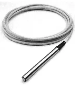
Figure 2.4: Global Water WL300 Water Level Sensor

For the Smartwells project, we are using the WL300 Water Level Sensor from Global Water Instrumentation Inc. which provides highly accurate water level measurements for a wide variety of applications in severe environments. The Water Level Sensor has a dynamic temperature compensation system which uses an internal thermister, enabling high accuracy measurements over a wide temperature range. The submersible pressure transducer is easily adapted to the Field Point module from National Instruments. The transducer is easy to install and operate. The Sensor has a two-wire high level 4-20 mA output. Full scale water level ranges are 0-3', 0-15', 0-30', 0-60', 0-120' and 0-250'.

The WL300 submersible pressure transducer is fully encapsulated with marine grade epoxy. The electronics are encased in epoxy so that moisture can never leak in through the 0-ring seals or work its way down the vent tube to cause drift or sensor failure (as is the case with other sensors). The vent tube is sealed directly to the sensing element and any moisture that may come down the vent tube will only come in contact with the silicon sensing device and not electronics.

(21)

The WL300 submersible pressure transducer uses a unique silicon diaphragm to interface between the water and the sensing equipment. This silicon diaphragm is highly flexible and is in intimate contact with the sensing element, which produces a sensor with exceptional linearity and very low hysteresis. Other metal foil diaphragms tend to crinkle and stretch out over time causing drift, linearity and hysteresis problems. The design of the Water Level Sensor eliminates these problems.

The pressure transducer is available in a 0-3' full scale range which is ideal for measuring shallow flows or small water level changes. The 0-3' range is great for measuring flows in sewers, storm drains, weirs, flumes, lakes, tanks or any water body that is less than 3' deep. The

0-3' sensor accurately measures small changes in water, even when water is only a few inches

deep. Other metal foil type sensors typically have serious problems at low level ranges because of crinkling, stretching and drifting.

The Water Level Sensor utilizes a stainless steel micro screen cap to protect the sensing element. This protective cap has hundreds of openings, making it virtually impossible to foul the sensor with silt, mud or sludge.

The WL300 submersible pressure transducer has a two-wire 4-20 mA output signal that is linear with water depth. 10 to 40 VDC is required to run the sensor, so the WL300 transducer can be operated from 12 VDC battery systems. The 4-20 mA signal can run up to 3,000' from the sensor to the logging device. Common twisted pair or electrical extension cord wire may be spliced to the vented cable once the cable is out of the water. The 4-20 mA signal may be converted to 0.5 to 2.5 VDC by dropping the current signal across a 125 ohm resistor.

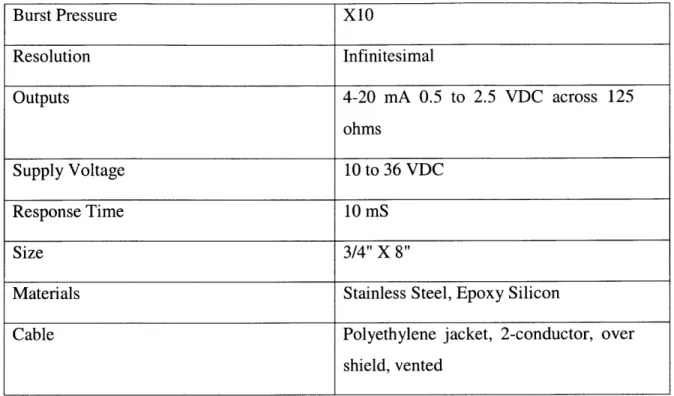
Specifications:

Pressure Range 0-3', 0-15', 0-30', 0-60', 0-120',0-250'

Linearity and Hysteresis ±0.1% FS

Overall Accuracy ±0.2% (35 0F to 700F)

(22)

Burst Pressure X10 Resolution Infinitesimal Outputs 4-20 mA 0.5 to 2.5 VDC across 125 ohms Supply Voltage 10 to 36 VDC Response Time 10 mS Size 3/4" X 8"

Materials Stainless Steel, Epoxy Silicon

Cable Polyethylene jacket, 2-conductor, over

shield, vented

Table 2.1 Specifications for water level sensor WL300

The submersible pressure transducer may be placed slightly below the lowest expected water level (this is not necessarily the total water depth) and the lowest possible range may be selected to cover the maximum expected water level change.

2.2.2 Conductivity Sensors

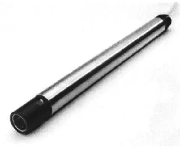
The conductivity sensors used in the Smartwells project were WQ301 Conductivity Sensors from Global Water Instrumentation Inc.

The conductivity sensor has two stainless steel electrodes. The outside electrode is a ring and the inside electrode is a wire. The conductivity sensor measures the ability of a solution to conduct an electric current between the two electrodes. The sensor can be used to measure either solution conductivity or total ion concentration of aqueous samples.

The conductivity sensor is automatically temperature compensated using an internal thermister. This means that one sample can be used for measurements in water samples of different temperatures. Without temperature compensation, the conductivity readings would change as the temperature changed, even though the actual ion concentration did not change.

(23)

Figure 2.5: Global Water Conductivity Sensor

For the calibration of the conductivity sensor, fill one container with tap water and another with a 5mS solution (where 1 Siemen, the unit of conductivity, is the reciprocal of the resistance in ohms measured between opposite faces of a centimeter cube of an aqueous solution at a specified temperature). Place the conductivity sensor in the latter container; turn on the power supply and the current meter. Let the sensor stabilize for 5 minutes before taking any measurements. Record the output current of the sensor, say X. Remove the sensor and rinse it off with tap water. Fill a contained with distilled water and repeat the above procedure to get an output current, say W. The lower current value for the sensor is equal to W, the output current the sensor would produce if the conductivity were 0. The high current value for the sensor is W, the output current produced if the conductivity is 5 ms. Using the new current values to recalibrate the system which is monitoring the sensor output, we get for some current output Y from the sensor, the corresponding conductivity obtained from the linearity of the sensor is

C =5000

opS

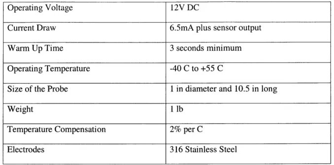
X - W Specifications:

Output 4-20 mA

Range 0 - 5 mS

(24)

Operating Voltage 12V DC

Current Draw 6.5mA plus sensor output

Warm Up Time 3 seconds minimum

Operating Temperature -40 C to +55 C

Size of the Probe 1 in diameter and 10.5 in long

Weight 1 lb

Temperature Compensation 2% per C

Electrodes 316 Stainless Steel

Table 2.2 Specifications for conductivity level sensor

2.2.3 Tipping Bucket Rain Gauge

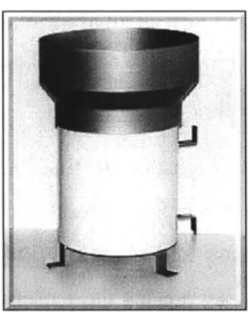
The Tipping Bucket Rain Gauge is a durable low-maintenance weather instrument for monitoring rain rate and total rainfall. It was designed by the National Weather Service to provide a reliable, low-cost tipping bucket rain assessment. Its simplicity of design assures trouble-free operation, yet provides accurate rainfall measurements. For the Smartwells project, we have sourced the rain gauge RG600 from Global Water Instrumentation Inc. which comes with a pulse logger RG700.

The RG600 unit has an 8" orifice and is shipped complete with mounting brackets and 50' of two-conductor cable. The tipping bucket mechanism activates a sealed reed switch that produces a contact closure for each 0.01", 0.2 mm or 1 mm of rainfall. The sensor consists of a gold anodized aluminum collector funnel with a knife-edge that diverts the water to a tipping bucket mechanism. The aluminum housing is covered with white baked enamel. The mechanism is designed so that each tip of the tipping bucket measures 0.2mm or 0.01 in of rainfall. A magnet is attached to the tipping bucket which actuates a magnetic switch as the bucket tips. Thus, a momentary switch closure takes place with each tip of the bucket. The

(25)

sensor is connected to an event/pulse counter on an electronic data logger, thereby keeping record of the accumulated rainfall.

The tipping bucket requires a clear and unobstructed mounting location to obtain accurate rainfall readings. The surface should be flat and the environment should be free of vibration. The tipping bucket should be calibrated with the rate of flow of water through the tipping bucket mechanism. At least 36 seconds should be allowed to fill one side of the tipping bucket, representing a maximum flow of 1 inch of rain per hour. If the flow rate is increased, then the unit will read low, since during the last 50% of the tipping time (the time it takes for the bucket to tip), water flows into the empty bucket. Decreasing the rate of flow will not affect the calibration. At flow rates of one inch an hour or less, the water actually drips into the bucket rather than flowing. Under these conditions, the bucket tips between drips and there is no error in the readings.

Figure 2.6: Global Water Rain Gauge RG600

Specifications

Resolution 0.01 in

Accuracy ±1% at 1" per hour

Average switch closure time 135 ms

Maximum Bounce settling time 0.75 ms

(26)

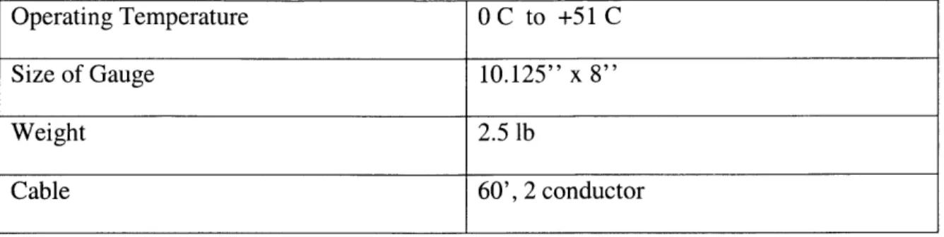
Operating Temperature 0 C to +51 C

Size of Gauge 10.125" x 8"

Weight 2.5 lb

Cable 60', 2 conductor

Table 2.3 Specifications for Rain Gauge RG600

The RG700 is a pulse logger whose output corresponds to the number of tips occurring in the RG600. The RG700 is essentially a capacitive circuit which resets each minute. The amount of rainfall in each minute can be logged corresponding to the number of tips in that minute.

Once sensors are selected for an instrumentation problem, the next issue is to read information from the sensors and process it. This is done using data acquisition hardware, some of which are discussed in this section.

The (analog) signals from the sensors are first usually processed by a signal-conditioning unit, which pre-processes the signal before it reaches the data acquisition hardware. It performs amplification, voltage stabilization and common filtering tasks like noise removal and anti-aliasing. The signal conditioner also powers the sensors whereby a separate power source for the sensors becomes unnecessary.

The conditioned signal is passed to the data acquisition hardware where it is converted from analog to digital by sampling it at a predetermined sampling frequency. The sampled digital output is then fed into the computer. The effectiveness of the data acquisition hardware depends primarily on its resolution and sampling rate. The resolution determines the number of bits used to represent an analog signal and the sampling rate determines the rate at which the continuous analog signal is discretized.

For the Smartwells project, the data acquisition hardware must be capable of acquiring data, buffering it, and transmitting the data to a central server on request. An integrated signal conditioning unit with data acquisition capabilities and sufficiently high resolution and sampling rates would be ideal. A variety of sensor inputs should be acceptable, the unit should be

(27)

low-maintenance and rugged enough for use in harsh environments. The network modules should support protocols.

The FieldPoint distributed data acquisition system, manufactured by National Instruments

was found to be suitable for the project. It comes with its own high level C library that can be easily interfaced with the feature-laden software development environment from National Instruments, making it very easy to write the data acquisition software.

2.3 Field Point Data Acquisition System

The FieldPoint system is a modular distributed 1/0 system. It allows easy software

integration and is one of the most cost-effective instruments available in the market. It is easy to configure, build and maintain reliable distributed I/O solutions. The FieldPoint system includes a variety of isolated analog and digital I/O modules, terminal bases, and network interfaces for an easy connection to open, standard networking technologies.

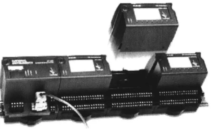
Fig 2.7 Complete FieldPoint Data Acquisition System - National Instruments

The sensor input modules accept a wide variety of sensor outputs at different sampling rates and bit resolutions. The network module then communicates with the host computer using RS 232 or TCP/IP to transfer data. FieldPoint supports plug-and-play customization of sensor input modules which makes it modular and easily upgradeable. This chapter discusses the 1/0 and network modules used in the Smartwells project in detail.

(28)

2.3.1 Input-Output (I/O) module:

Two general I/O modules - standard 8/16 channel modules and the dual-channel modules are available with the FieldPoint installation. The FP-Al-110 modules support up to eight channels of voltage or current inputs with 16 bit resolution. The FP-AI- 110 module is an analog input module with eight analog input channels. The FP-Al-i 10 is ideal for low frequency signals, and has three configurable filter settings to reject noise. User programmable low-pass filters at 50, 60 and 500 Hz settings are available. Hot plug and play operation, safety isolation, and the 11 input ranges ensure that installation and maintenance are as trouble free as possible.

Fig 2.8 FP-AI-110 I/O Module - National Instruments

Specifications:

Table 2.4 Specifications for FP-AI-110 I/O Module

Number of channels 8

ADC Resolution 16 bits

Type of ADC Delta-Sigma

Safety isolation/Working Voltage 250 V rms, designed per IEC 1010 as

(29)

The speed of data transfer between the FieldPoint module and the host computer depends upon two independent factors, the sampling rate of the sensor input module and the network

throughput rate. The sampling rate of the module is defined as the rate at which the ADC

(Analog-Digital Converter) in the module digitizes the input and places it in the output register. This is independent of the number of active channels in the module and depends only on the low-pass filter setting. The sampling rates for the FP-Al-110 module are summarized in the following table.

REJECTION FREQUENCY SAMPLING RATE

50 Hz 1.47 sec

60 Hz 1.23 sec

500 Hz 0.17 sec

Table 2.5: Sampling Rates for FP-AI-110

2.3.2 Network Module:

The network modules communicate with the local 1/0 module via the high-speed local bus formed by linked terminal bases. The FP-1600 network interface module from National Instruments provides an easy compatible connectivity solution. It connects a node of up to nine

(30)

Fig 2.9 FP-1600 Network Module - National Instruments

The FP-1600 is a bare bones Ethernet module without any onboard memory buffer. It supports both 10 and 100 Mb/s data transfer rates, the actual speed being auto-negotiated depending on the network. Each FP-1600 module can support up to nine sensor input modules.

Specifications:

Network Interface l0BaseT and l00BaseTX Ethernet

Compatibility IEEE 802.3

Communication Rate 10Mbps, 100Mbps, auto-negotiated

Power Supply Range 11 to 30 volts DC

Power Consumption 7 W + 1.15 (Power for 1/0 Modules)

Operating Temperature 0 to 55 deg. C.

Dimensions 10.9 by 10.9 by 9.1 cm

Weight 250g

(31)

The FP-1600 module can be configured using the FieldPoint Explorer program available from National Instruments. Configuring the device involves assigning an IP address and configuring the modules attached to it. The FieldPoint module and the computer used for the configuration should be on the same class B subnet and have a subnet mask of 255.255.0.0. The configuration can then be saved as an IAK (Industrial Automation Kernel) file, which can be

accessed by National Instruments software like Measurement Studio.

The network throughput rate is the rate at which the network interface module transfers

data between the FieldPoint module and the host computer. This depends on a number of factors such as network traffic, total number of channels in the installation (but not on the number of modules itself), FieldPoint processing time, etc. The time taken for the network module to read data from the sensor input modules is negligible compared to the sampling rate of the I/O module and the network throughput rate of the network module. The following table shows some typical transfer rates for the FP-1000 module connected to one analog input module, such as FP-AI-1 10.

BAUD RATE

115.2 57.6 38.4 19.2 9600 b/s

I Channel 6 ms 9 ms 11 ms 19 ms 34 ms

4 Channels 9 ms 12 ms 16 ms 27 ms 49 ms

8 Channels 12 ms 17 ms 22 ms 37 ms 68 ms

Table 2.7 Transfer Rates for FP-1000 [with FP-AI-110 I/O module]

The overall sampling rate is determined by whether the network throughput rate or the sampling rate actually governs.

2.4 Data Collection

The next part of the system involves wireless transmission of the data to the data server wirelessly via a wireless network card, central router and then archiving it in a database. The central wireless router and the wireless network cards use 802.11 .b protocol for the wireless

(32)

transmission and receiving of data. A data server running LabWindows/CVI collects the data transmitted from the FieldPoint module. LabWindows is a data collection and visualization software package created by National Instruments to interface with the FieldPoint module. The LabWindows software makes use of the CVI ('C' for virtual Instruments) programming language to collect and display data. Once the data server receives the data, a data socket is written so that other programs have access to it. A Data Sockets Server broadcasts data over TCP/IP sockets using the multithreaded DataSocket API. Data sockets are similar to the normal sockets i.e. they are temporary storage locations that package the data transmission and make it available to external computers. While the data is constantly being streamed through on the data socket, a copy of that data is sent to a database and a web server which resides on the same machine for the purpose of the Smartwells project. The client side code for retrieving data from a

DataSocket server and techniques to write data to the database and retrieve data from it are

reviewed later in this chapter. The following section gives us specifications of the wireless technology and devices used.

2.4.1 Wireless Architecture

For the purpose of the Smartwells project, the sensors are physically connected to a data

acquisition device in their proximity and a wireless link between the host computer and multiple data acquisition devices is used for data transfer. The data acquisition device has its own networking and processing capabilities in the case of the FieldPoint module.

The wireless devices used were off-the-shelf wireless solutions from Orinoco Wireless, Lucent Technologies. These devices use the 2.4-2.485 GHz spectrum for communication and enable data transfer using the IEEE 802.11 b (also called WiFi) protocol with data transfer rates of up to 11 Mbps. A FieldPoint module and a host computer connected to individual wireless network cards communicate via a central router called the Residential Gateway. While the range of the wireless cards is variable, the residential gateway provides up to 150 m of roaming access in the straight line of sight. In enclosed spaces such as the Design Studio in Building I at MIT, this range was found to be around 40m. The last part of the wireless network topology is the Ethernet converter that takes serial or Ethernet inputs and connects to a wireless network card.

(33)

This wireless infrastructure was found to be quite feasible for the Smartwells project due to the low sampling rates needed for level, rainfall and conductivity probes. The data flovxs from the

FieldPoint module to the Ethernet converter, then to the central router i.e. the Residential

Gateway via the wireless network card and finally to the host computer hosting the data acquisition server via a wireless network card.

Browser Residential

Gateway

Wirele Ethernet and serial Converter

LAN 802.11b

Data Server

Also the APP and WEB Server FieldPoint Data

Acquisition

Fig. 2.10 Wireless System Architecture

A Lucent Wireless - Orinoco Residential Gateway (Model RG1000) was used with

Orinoco Silver PC cards and 1OBase-T Ethernet converter.

2.5 Software for Data Acquisition

The Smartwells project implements a distributed data acquisition and processing system which comprises of the data server, application server and the web server. For the purpose of the

Smartwells project, all these parts of the distributed data acquisition architecture sit on the same

physical machine http://smartwells.mit.edu. Later, we consider the issue of archival of real-time data and retrieval of this archived data.

(34)

The FieldPoint sensor input modules sample the data from the sensors and communicate

it to the rwork interface module of the installation. -The host computer accesses and processes this data by polling the instrument through Ethernet. National Instruments provides a highly compatible software solution 'Measurement Studio' to go with its FieldPoint module installations, thereby alleviating the need for socket-level programming. The Measurement Studio software suite comes with LabWindows/CVI, a component which is an ANSI C compliant programming interface.

LabWindows CVI has a convenient interface to FieldPoint network modules and comes with significant signal processing capability and provision to spawn off external Java programs. This data acquisition software is discussed in more detail further in this chapter.

Data from the six sensors - two level sensors, two conductivity sensors and two rain gauges is sampled at a low frequency of 1 Hz. The low frequency chosen proves to be sufficient because there is not a substantial change in hydrological data measured by these sensors within this time frame. Also, the full load of processing the acquired data falls on the host computer due to lack of on-board memory buffers in the network module. It is seen that the machine can easily handle the load of database archival and retrieval due to the low sampling frequency chosen. The data acquisition CVI server runs on the same machine as the database (SQL Server 2000), application and web server (Apache on Port 80 and MS-IIS 6.0 with ASP.NET on Port 81). The same machine also hosts the National Instruments DataSocket server (which hosts data published

by the CVI server) and a separate archival process (which archives this real-time data).

This setup allows an applet hosted on the web server to access both real-time data from the data acquisition server as well as archived data from the database server. The table below lists the services running on the Smartwells server:

SERVICE DESCRIPTION

CVI Collects data from the FieldPoint installation and Server (menu.exe) publishes it to a DataSocket server

Da taSocket Server _{National Instruments DataSocket server}

(35)

Archival Process Archives the real time data from the DataSocket (Archive. class) Server by writing it to the SQL Server Database Database Server Runs a Database server for data archival and stored

(MS-SQL Server) procedures to query field data

ASP .NET Web server running on port 81 serving ASP.NET

(with MS-IIS 6 . 0) _{pages that access archived data from the SQL}

Apache (with Web server running on port 80 and servlet runner

Tomcat) that access real-time and archive data from the

Table 2.8 Services running on the Smartwells server

2.5.1 LabWindows/CVI Interface

The steps involved in data acquisition from the FieldPoint module with the help of the LabWindows/CVI server are discussed in this section.

-r-IEI F* 01DW l VO r11118* _______________________________________________ H I IA Server wth OPC n- #FieldPoint [- FP Ries FP- 1600 0 Charnel 0 Channel I SCharnie 3 Channel 4 Chwnnel 5 Channiel 6 Chariel 7 J# Irpt Fier @Ch2 tt+ FP-TB-10 @2 141 1211 R88tdy ~

Fig 2.11 FieldPoint Explorer configuration

I Al *Chaerl 0 &Chanel 1 &'Chanel 2 Channel 3 &Charnel 4 Chamel 5 Channelo 6 Channel 7 Snput Fier @Ch2 +0.001348 +0,001348 +0.001883 +0.001349 -0.000000 +0.000000 +0.000000 OOFF 0001 0002 0004 0010 0020 0040 0000 0004:0001 d R t 23:53:51:941 23:53:51:941 23:53:53:331 23:53:52:246 23:53:49:938 23:51:28:181 23:51:25:785 rutih-dwnel tern -0.021 to 0.021 amps -0.021 to 0.021 amips -0.021 to 0.021 amps -0.021 to 0.021 amrps -0.021 to 0.021 amfps -0.021 to 0.021 amtips -0.021 to 0.021 amrps -0.021 to 0.021 amps 0.0 to 255.0 Successfill Successl ci Successfil SuccessfUlc Successfdi Task is terminated. Task is terminated. ucccessfl! Successfli! SuccessfuL! 100 msec 100 msec 100 msec 100 mscc 100 msec 100 msec 100 mec 100 msec 100 msec 100 msec foat foat foat foat foat foat float foat float 4-byte Lint NUM 3CR I Add rs- I., -- | k A t I A- 5 I - ae I t 9W I

(36)

The FieldPoint Explorer program provided by National Instruments is used to configure the FieldPoint module and the module configuration is saved in an IAK file. Following this, the

instrument libraries are loaded into CVI enabling the data acquisition code to call methods provided by these instrument interfaces. A snapshot of the Field Explorer configuration is presented in Fig.2.11.

In order to talk to the FieldPoint module, we get a socket handle to the instrument using

the FPOpen() function. This functionality is embedded inside the startMonitoring() function in the myfunctions.c available on the Smartwells website. Next, the startMonitoring() function gets

a handle over all the channels that need to be monitored using the FPCreateTagIOPoint() call to which we pass the instrument handle, instrument name, channel to monitor and a channel handle as parameters.

/* Open a FP Connection

if (status = FPOpen (NULL, &FP handle)) {

Error(status);

* Code to create an advise operation for each of the sensor annels */ for(i=0; i<numChannels; i++){

if (status = FPCreateTagIOPoint(FP handle, 'FP Res",module[0], itemName[i] ,&I0 handle[i]))

Error(status);

if (status = FPAdvise (FPhandle, IOhandle[i], 100, 0, advisebuf[i],

100, 1, NULL, NULL, &advise_ID[i]))

Error(status); }

The channel handle is then used to poll the instrument using FP Advise() which takes as its parameters the instrument handle, the channel handles, the advise rate ( instrument polling rate), a global array to hold the channel data, a notify-on-change flag, an array buffer to cache data, buffer size in bytes, callback type flag, an optional callback function (triggered when the memory buffer gets written to), a callback event notifier and a data handle. An interface for editing the Advise operators and the module settings is presented in Fig.2.12.

Notify-on-change callbacks may be used for monitoring slow events. But since the

Smartwells machine single-handedly runs all the necessary servers, such callbacks may put undue load on the machine. Instead, we use a timer to process the buffered data. This timer calls its callback function after each period and reads data off the memory cache into the data handle. Though a UI timer provided by CVI could have been used due to the low advise rates, an asynchronous timer object borrowed from the MIT Flagpole project was used in case some

(37)

additional sensors requiring high sampling rates were added on later. This timer makes system-level calls to the OS and works satisfactorily even for high sampling rates.

*~ I M*~ q%~@ ~

AJ,

wi~fr2 PM"

Fig. 2.12 Interface using CVI

The timer frequency is retrieved from the panel (in the example, the frequency is 1Hz) and is followed by the instantiation of an asynchronous timer. The callback function adviseCB is triggered after each period. The period is the first argument passed to the asynchronous timer instance.

/* initialize async timer *

GetCtrlVal(panelHandlePANELNUMERICRNOB,&frequency);

timerID = NevAsyncTixer (1.00/frequency, -1, 1, adviseCB, 0);

Finally, data from the cache is read using the FPReadCache () method which takes in an

instrument handle, an advise operation, a data holder, buffer size and a pointer to a time stamp structure as its parameters.

(38)

if ( !DEBUG){

is = FP_ReadCache(FPhandle, advise_ ID[i],current_read, BUFFERSIZE,&dummy);

value = (float*)(currentread);

/* (ule)(*va!ue)*scale.F Actor[ i-zeroVtage[ i)/ens tiviti] */

channels[i][counter] = (double)(*value); }else channels[i][counter] = i+rand(/(2*32767.0); if (voltpanel) SetCtrlVal(voltpanel,VOLTPANELCHANNEL_0-ichannels[ i][counter]); }

A system timer is used for timing the data that is then cast as a pointer to float and dereferenced

to get the final float value. This data is now made available using the DataSocket APIs. The data acquisition server can be configured using XML-like configuration file which contains, in addition to other options, the number of channels to be monitored in the FieldPoint module.

2.5.2 DataSockets API

The Smartwells project uses the DataSocket API implementation for LabWindows / CVI for sharing real-time data. The National Instruments DataSocket Server/API uses the

publisher-subscriber model (Fig. 2.13) for sharing real-time data as opposed to a client-server one.

In real-time data applications, the server cannot be burdened with thread generation, handling and termination tasks. The DataSocket API uses the publisher-subscriber model in which the publisher writes serialized data to a dedicated socket from where it is accessible to all the subscribers. The API takes care of forking multiple connections and uses reflection to enabling dynamic data type recognition of deserialized data at the subscriber end.

To write the data to a DataSocket server from LabWindows/CVI, we get a handle to the

DataSocket URI (in our case, dstp://smartwells.mit.edu/data) and then use the DSOpen()

function call from the API to post data to this URI. After getting the DataSocket URI, the

DSOpen() function used for posting data takes as its parameters the URI, a connection type, a

callback type, optional parameters to pass to the callback function and a handle to the

DataSocket connection.

GetCtr1Va1(pane1Hand1e,PANEL_R INGURL);

DSOpen (URL, DSConstWriteAutoUpdate, DSCallback, NULL, &dsHandle);

An automatic update to the server is preferred every time data gets written, and hence the

(39)

LAB WINDOWS / CVI

Data Acquisition Server Applet Subscriber

dstp://smartwells.mit.edu/data

DataSocket Server/API

Fig. 2.13: DataSocket Model

A Callback function for DataSocket events is then triggered with every status change at the

server. The DSOpen() function then takes an optional parameter that is the data to be passed to the callback function (in our case, NULL). The final parameter passed is a handle to the

DataSocket connection. Upon successful connection, data may be written to the DataSocket

server via a callback to the asynchronous timer (adviseCB). Instead of publishing data at the end of each advise operation, data is published in cycles each consisting of 10 advise operations on the 1/0 modules. The Windows time-stamp is converted to a Java time-stamp using the following code:

static unsigned long secondsDiff = 2208988800;

switch (event){

case EVENT_TIMERTICK: GetLocalTime(&dummy);

localTimeInSeconds time(NULL);

localTimeInMillis = (localTimeInSeconds-secondsDiff )*1000 .0+dummy.wMilliseconds;

The data is written to a DataSocket server as a 2D array using a call to the DSSetData Value() function.

(40)

if (counter == 10){ if (dsHandle){

hr = DSSetDataValue (dsHandle, CAVTDOUBLEICAVTARRAY, channels, numChannels+1, 10);

}

counter = 0;

This function takes as its parameters a handle to the DataSocket connection, an object type for data written to the server, the 2-D array being eventually written to the server, the number of rows and the number of columns. The data thus published by the Publisher can then be accessed

by several subscribers by binding the DataSocket URI.

2.5.3 Archiving Data

The software framework for archiving the obtained data is now discussed. As mentioned earlier, the data archiving program runs on the web server, which is distinct from the data

acquisition server.

The data is archived in a MS-SQL Server 2000 database which runs on the Smartwells machine. The snapshot of the table layout can be seen in Fig. 2.14. The stored procedures run database queries to extract specific well or precipitation data for a required time frame using Transact SQL (for SQL Server Enterprise Manager) / Standard SQL (for Java Archival process) and return datasets of the results.

The data model for the Smartwells database can be seen in Fig.2.15. The database has 3 tables, one each for level, conductivity and rainfall linked together by the instant of data collection as the primary key.

(41)

Fig 2.14 Table Layout for MS-SQL Server 2000 Smartwells Database Conductivfty Rafafl I Indexer Sindexer WelCond .._DateTime WeIlCond2 Guagel DateTime Guage2

(42)

The database access and archiving code is now discussed further.

Database Access and Archival Process

The JDBC-ODBC driver that comes along with the JDK was used for primary database access. The code was optimized to minimize the number of database connections created and persistent connections were ensured.

The archival program written in Java subscribes to the DataSocket server, listens for updates, writes the updates to a text file and then does a bulk insert of text data into the SQL Server database every minute. The details of this task are delineated in this section.

The Archive constructor instantiates a DataSocket, binds it to the Smartwells URI opening the connection as a Subscriber. The access mode is set to cwdsReadAuto Update so that callback is triggered each time new data becomes available or when the connection status changes. An event listener associated with this DataSocket calls the writeData() function on every update to the DataSocket instance. The code snippet corresponding to these tasks is shown below: ds = new DataSocket(); ds.setURL(" p ds.setAccessNode(DSAccessModes.cwdsReadAutoUpdate); ds.setAutoConnect(true); ds.addDSOnDataUpdateListener(new DSOnDataUpdateListener() {

public void DSOnDataUpdate (DSOnDataUpdateEvent even) {

writeData (event);

On each call, the writeData() function reads the data from the DataSocket as a 2D array of doubles with entries corresponding to each channel monitored and the time stamp. Since the

DataSocket gets written to after 10 advise cycles, each call to writeData() gets 10 entries. This

(43)

DSData fDatua = ds.getData();

double reLdatc1a[] try {

readData = f Data. GetValueAsDoubleArray2D );

for (int i=O;i<10;i++){

out. pr int ln (readData[ O] [i] +", "+

readData[1] [i]+" "+ readData[2] [i]+" "+ readData[3] [i]+" "+ readData[4][i]); }

The PrintWriter is flushed and closed each minute and a bulk insert is done on the SQL Server

database. A new PrintWriter is again instantiated as seen:

minute = Calendar.getInstance () .get (Calendar.MINUTE); if(minute != currentMinute)( currentMinute = minute; out.flush(); out.closef(; out = mnl1; try stt = con.createStatemento;

String statewenu = >ul-i"+FILENAME+f' VIUI FD I ;

System.out.println(statement); stmt.executeUpdate(statement);

}cat ch(SQLException c2){ e2.printStackTrace();

try

out = new Printriter(new Fileriter(FILENAME,false) , true); // open new buffer

A function which starts up and shuts down the DataSocket connection is shown in the following

code snippet:

public void startListening() (new File(FILENAME).delete();

ds. connect );

public void stopListening() {

ds.disconnect();

2.5.4 Data Visualization

This section describes the applets developed for data visualization and rendering. There are two kinds of data rendered - real-time data and archived data. The real-time data is rendered

(44)

using applets which subscribe to the DataSocket server to fetch real-time data (just like the Archive program). The archived data is rendered using applets which query the SQL Server database to extract data. Smartwells project also implements a web service to extract archived data using ASP.NET. Chapter 5 details more about this web service and its architecture. Some of the applets developed for the Smartwells project are mentioned below:

The real-time water level monitoring applet subscribes to the DataSocket server

This applet uses the DataSocket API from National Instruments to display real time water level information in two prototype wels. In the future, sensors wilt be added to measure other parameters like pH, etc.

Fig 2.16 Water Level Monitoring Applet

and displays well information (water-level, conductivity, flow rate and temperature out of which the first two sensors are available) for two sample wells being monitored. The well properties in the two wells in the applets can be seen changing in real-time with any change in the actual well properties. The blue level in the applet wells shows the scaled water level in each well so as to give zero water level for an actual 2" level and full water level for a head of 30".