Data, Models and Decisions for Large-Scale
Stochastic Optimization Problems
by
Velibor V. Mišić
B.A.Sc., University of Toronto (2010)
M.A.Sc., University of Toronto (2012)
Submitted to the Sloan School of Management
in partial fulfillment of the requirements for the degree of
Doctor of Philosophy in Operations Research
at the
MASSACHUSETTS INSTITUTE OF TECHNOLOGY
June 2016
c
○ Massachusetts Institute of Technology 2016. All rights reserved.
Author . . . .
Sloan School of Management
May 10, 2016
Certified by . . . .
Dimitris Bertsimas
Boeing Professor of Operations Research
Co-Director, Operations Research Center
Thesis Supervisor
Accepted by . . . .
Patrick Jaillet
Dugald C. Jackson Professor of Electrical Engineering
and Computer Science
Co-Director, Operations Research Center
Data, Models and Decisions for Large-Scale Stochastic
Optimization Problems
by
Velibor V. Mišić
Submitted to the Sloan School of Management on May 10, 2016, in partial fulfillment of the
requirements for the degree of
Doctor of Philosophy in Operations Research
Abstract
Modern business decisions exceed human decision making ability: often, they are of a large scale, their outcomes are uncertain, and they are made in multiple stages. At the same time, firms have increasing access to data and models. Faced with such complex decisions and increasing access to data and models, how do we transform data and models into effective decisions? In this thesis, we address this question in the context of four important problems: the dynamic control of large-scale stochastic systems, the design of product lines under uncertainty, the selection of an assortment from historical transaction data and the design of a personalized assortment policy from data.
In the first chapter, we propose a new solution method for a general class of Markov decision processes (MDPs) called decomposable MDPs. We propose a novel linear optimization formulation that exploits the decomposable nature of the problem data to obtain a heuristic for the true problem. We show that the formulation is theoretically stronger than alternative proposals and provide numerical evidence for its strength in multiarmed bandit problems.
In the second chapter, we consider to how to make strategic product line decisions under uncertainty in the underlying choice model. We propose a method based on robust optimization for addressing both parameter uncertainty and structural uncer-tainty. We show using a real conjoint data set the benefits of our approach over the traditional approach that assumes both the model structure and the model parame-ters are known precisely.
In the third chapter, we propose a new two-step method for transforming lim-ited customer transaction data into effective assortment decisions. The approach involves estimating a ranking-based choice model by solving a large-scale linear op-timization problem, and solving a mixed-integer opop-timization problem to obtain a decision. Using synthetic data, we show that the approach is scalable, leads to ac-curate predictions and effective decisions that outperform alternative parametric and non-parametric approaches.
personalized assortment decisions. We develop a simple method based on recursive partitioning that segments customers using their attributes and show that it improves on a “uniform” approach that ignores auxiliary customer information.
Thesis Supervisor: Dimitris Bertsimas
Title: Boeing Professor of Operations Research Co-Director, Operations Research Center
Acknowledgments
First, I want to thank my advisor, Dimitris Bertsimas, for his outstanding guidance over the last four years. Dimitris: it has been a great joy to learn from you and to
experience your unbounded energy, love of research and positivity, which continue to amaze me as much today as when we had our first research meeting. I am extremely
grateful and indebted to you for your commitment to my academic and personal development and for all of the opportunities you have created for me. Most of all,
your belief in the power of research to have impact has always been inspiring to me, and I shall carry it with me as I embark on the next chapter of my academic career.
I would also like to thank my committee members, Georgia Perakis and Retsef
Levi, for providing critical feedback on this research and for their support on the academic job market. Georgia: thank you for your words of support, especially at a
crucial moment early in my final year, and for all of your help, especially with regard to involving me in 15.099, providing multiple rounds of feedback on my job talk and
helping me prepare for pre-interviews at INFORMS. Retsef: thank you for pushing me to be better, to think more critically of my work and for suggesting interesting
connections to other research.
I have also many other faculty and staff at the ORC to thank. Thank you to the
other faculty with whom I interacted and learned from during my PhD: thank you Patrick Jaillet, Juan Pablo Vielma, David Gamarnik, Jim Orlin, Tauhid Zaman and
Karen Zheng. In addition, I must thank the ORC administrative staff, Laura Rose and Andrew Carvalho, for making the ORC a paragon of efficiency and for always
having a solution to every administrative problem or question that I brought to them.
I would also like to acknowledge and thank my collaborators from MIT Lincoln Laboratories for their support: Dan Griffith and Mykel Kochenderfer in the first two
years of my PhD, and Allison Chang in the last two years.
The ORC community has been a wonderful home for the last four years, and I was extremely lucky to make many great friends during my time here. In
Thraves, Stefano Tracà, Alex Weinstein, Miles Lubin, Chiwei Yan, Matthieu Monsch, Allison O’Hair, André Calmon, Gonzalo Romero, Florin Ciocan, Adam Elmachtoub,
Ross Anderson, Vishal Gupta, Phebe Vayanos, Angie King, Fernanda Bravo, Kris Johnson, Maxime Cohen, Nathan Kallus, Will Ma, Nataly Youssef, David Fagnan,
John Silberholz, Paul Grigas, Iain Dunning, Leon Valdes, Martin Copenhaver, Daniel Chen, Arthur Flajolet, Zach Owen, Joey Huchette, Nishanth Mundru, Ilias Zadik,
Colin Pawlowski and Rim Hariss. Andrew and Charlie: thank you for being there from even before the beginning and for many epic nights. Anna, Alex R. and Charlie:
thank you for being the best project partners ever. Alex S., Alex W. and Anna: I will never forget all the fun we had planning events as INFORMS officers. Vishal:
thank you for your mentorship during my first two years and for many insightful conversations on research and life in general. Maxime and Paul: thank you for an
unforgettable trip to upstate New York (and please remember to not keep things “complicated”)! Vishal, Maxime and Kris: thank you for your support during the job
market, especially in the last stage of the process. Nishanth: thank you for many cre-ative meetings for the TRANSCOM project that often digressed into other research
discussions. Nataly: thank you for your encouragement in difficult times and also for having plenty of embarrassing stories to share about me at social gatherings. Adam
and Ross: thank you for hosting me so many years ago and setting the right tone for my ORC experience.
I also had many great teaching experiences at MIT, for which I have many people
to thank. Allison: thank you for being a fantastic instructor and coordinator, and for your saint-like patience when I was a teaching assistant for the Analytics Edge in
its regular MBA, executive MBA and MOOC incarnations. Iain, John, Nataly and Angie: thank you for being great teammates on the 15.071x MOOC.
Thank you to the Natural Sciences and Engineering Research Council (NSERC) of Canada for providing financial support in the form of a PGS-D award for the first
three years of my PhD. Thank you also to Olivier Toubia, Duncan Simester and John Hauser for making the data from their paper [91] available, which was used in
I had the great fortune of making an amazing group of Serbian friends in Cam-bridge during my time at MIT. To Saša Misailović, Danilo Mandić1, Marija Mirović, Ivan Kuraj, Marija Simidjievska, Irena Stojkov, Enrico Cantoni, Miloš Cvetković, Aca Milićević, Marko Stojković and Vanja Lazarević-Stojković: thank you for everything.
I will miss the brunches at Andala and the nights of rakija, palačinke, kiflice, the immortal “Srbenda” meme, the incomprehensible arguments between Marija S. and
Kafka, and the MOST-sponsored Toscanini-induced ice cream comas.
I am also indebted to many friends outside of the ORC at MIT; a special thank
you to Felipe Rodríguez for being a wonderful roommate during the middle of my PhD and to Francesco Lin for being a great party and concert buddy. Thank you
Peter Zhang and Kimia Ghobadi for many great get-togethers to relive our old glory days at MIE (which reminds me: we still need to catch up!). Outside of MIT, thank
you Auyon Siddiq for being a great friend and for always helping me in my many dilemmas, and thank you Birce Tezel for your words of reassurance in hard times
and for helping me bounce gift ideas off you. I also need to thank my friends from my undergrad days in Toronto for being my biggest fans: thank you Eric Bradshaw,
Jordan DiCarlo, Geoffrey Vishloff, Lily Qiu, Torin Gillen, Emma Tsui, Oren Kraus, Archis Deshpande and Anne Zhang. Thank you also to Konstantin Shestopaloff for
many great lunches and inspiring conversations during my visits back to Toronto.
I would not have reached this point without the support of my family: my father
Vojislav, my mother Jelena, my brother Bratislav and my sister-in-law Elena. Thank you for your unwavering and unconditional love; words cannot express how grateful
I am to you for supporting me in my decision to come to MIT, for advising me in complex and delicate situations, for always being on my team, for making me feel
better after particularly rough days and for visiting me in Cambridge many times over the last four years. The best work in this thesis happened during my visits to
Toronto, when we would all be working on our own thing in the living room but together, and I always look forward to our next discussion, whether it is about what
happened in the latest episode of Game of Thrones or Državni Posao, or Meda and
Mačiko’s latest exploits. Which reminds me: I should also thank our quadrupedal companions, Mačiko2 and Meda3, for their contributions to this thesis.
Last but not least, I would like to thank my girlfriend Dijana, for her love and support, for being by my side at the lowest and the highest points of my PhD, for
always being positive and for reminding me that there is more to life than research, such as getting brunch on a Sunday at Tatte or going for a run along the Charles
River. Above all, thank you for making the last couple of years the happiest of my life. It is to her and my family that I dedicate this thesis.
2Also known as “Šmica”, “Dlakavo đubre”; a black cat of unknown provenance.
3Also known as “Kerenko”, “Keroslav”, “Kerenski”, “Skot”; a black lab-husky puppy. My walks
Contents
1 Introduction 19
1.1 Decomposable Markov decision processes: a fluid optimization approach 20
1.2 Robust product line design . . . 21
1.3 Data-driven assortment optimization . . . 22
1.4 Personalized assortment planning via recursive partitioning . . . 23
2 Decomposable Markov decision processes: a fluid optimization ap-proach 25 2.1 Introduction . . . 25
2.2 Literature review . . . 30
2.3 Methodology . . . 34
2.3.1 Problem definition . . . 34
2.3.2 Fluid linear optimization formulation . . . 35
2.3.3 Properties of the infinite fluid LO . . . 37
2.3.4 Fluid-based heuristic . . . 39
2.4 Comparisons to other approaches . . . 43
2.4.1 Approximate linear optimization . . . 43
2.4.2 Classical Lagrangian relaxation . . . 44
2.4.3 Alternate Lagrangian relaxation . . . 46
2.4.4 Comparison of bounds . . . 51
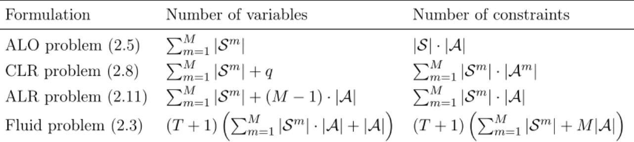
2.4.5 Comparison of formulation sizes . . . 52
2.4.6 Disaggregating the ALO and the ALR . . . 53
2.5.1 Problem definition . . . 55
2.5.2 Fluid model . . . 55
2.5.3 Relation to [19] . . . 56
2.5.4 Bound comparison . . . 59
2.5.5 Large scale bandit results . . . 61
2.6 Conclusion . . . 65
3 Robust product line design 69 3.1 Introduction . . . 69
3.2 Literature review . . . 73
3.3 Model . . . 77
3.3.1 Nominal model . . . 77
3.3.2 Robust model . . . 81
3.3.3 Choices of the uncertainty set . . . 86
3.3.4 Trading off nominal and robust performance . . . 90
3.4 Results . . . 91
3.4.1 Background . . . 93
3.4.2 Parameter robustness under the first-choice model . . . 95
3.4.3 Parameter robustness under the LCMNL model . . . 96
3.4.4 Parameter robustness under the HB-MMNL model . . . 100
3.4.5 Structural robustness under different LCMNL models . . . 103
3.4.6 Structural robustness under distinct models . . . 105
3.5 Conclusion . . . 110
4 Data-driven assortment optimization 111 4.1 Introduction . . . 111
4.2 Literature review . . . 116
4.3 Assortment optimization . . . 121
4.3.1 Choice model . . . 121
4.3.2 Mixed-integer optimization model . . . 123
4.5 Computational results . . . 130
4.5.1 Tractability of assortment optimization model . . . 131
4.5.2 Constrained assortment optimization . . . 132
4.5.3 Estimation using column generation . . . 138
4.5.4 Comparison of revenue predictions . . . 141
4.5.5 Combining estimation and optimization . . . 146
4.5.6 Comparison of combined estimation and optimization procedure 149 4.6 Conclusions . . . 153
5 Personalized assortment planning via recursive partitioning 155 5.1 Introduction . . . 155
5.2 Literature review . . . 157
5.3 Model . . . 160
5.3.1 Background . . . 160
5.3.2 Uniform assortment decisions . . . 161
5.3.3 Personalized assortment decisions . . . 161
5.4 The proposed method . . . 162
5.4.1 Data . . . 163
5.4.2 Building a customer-level model via recursive partitioning . . 164
5.5 Results . . . 167
5.6 Conclusion . . . 171
6 Conclusions 173 A Proofs, Counterexamples and Derivations for Chapter 2 175 A.1 Proofs . . . 175
A.1.1 Proof of Proposition 1 . . . 175
A.1.2 Proof of Proposition 2 . . . 176
A.1.3 Proof of Proposition 3 . . . 178
A.1.4 Proof of Theorem 1 . . . 178
A.1.6 Proof of Theorem 2 . . . 185
A.1.7 Proof of Theorem 3 . . . 188
A.1.8 Proof of Theorem 4 . . . 189
A.1.9 Proof of Proposition 9 . . . 194
A.2 Counterexample to show that 𝑍*(s) ≤ 𝐽*(s) does not always hold . . 197
A.2.1 Bound . . . 197
A.2.2 Instance . . . 198
List of Figures
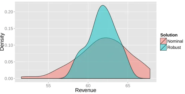
3-1 Hypothetical illustration of revenue distributions under two different
product lines. . . 84
3-2 Plot of revenues under nominal and robust product lines under boot-strapped LCMNL models with 𝐾 = 8. . . 98
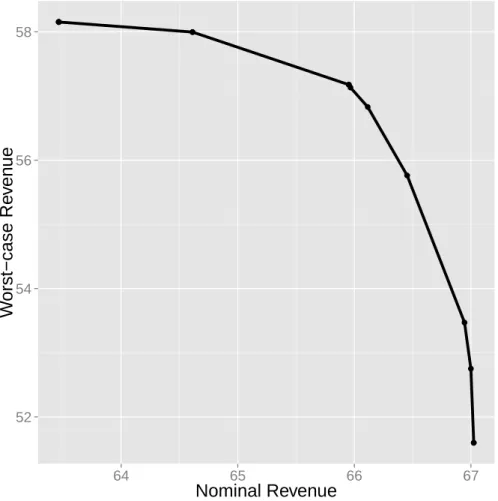
3-3 Plot of approximate Pareto efficient frontier of solutions that trade-off nominal revenue and worst-case revenue under the bootstrapped uncertainty set ℳ for 𝐾 = 8. . . 99
3-4 AIC for 𝐾 ∈ {1, . . . , 20}. . . 104
3-5 CAIC for 𝐾 ∈ {1, . . . , 20}. . . 104
3-6 First-choice product line, 𝑆N,𝑚FC. . . . 107
3-7 LCMNL model with 𝐾 = 3 product line, 𝑆N,𝑚LC3. . . . . 108
3-8 LCMNL model with 𝐾 = 12 product line, 𝑆N,𝑚LC12. . . . . 108
3-9 Robust product line, 𝑆R. . . 108
3-10 Competitive products. . . 109
4-1 Evolution of training error and testing error with each column gener-ation itergener-ation for one MMNL instance with 𝑛 = 30, 𝑇 = 10, 𝐿 = 5.0 and 𝑀 = 20 training assortments. . . 142
4-2 Evolution of optimality gap with each column generation iteration for one MMNL instance with 𝑛 = 30, 𝑇 = 10, 𝐿 = 5.0 and 𝑀 = 20 training assortments. . . 150
List of Tables
2.1 Comparison of sizes of formulations. (The number of constraints quoted
for each formulation does not count any nonnegativity constraints.) . 53
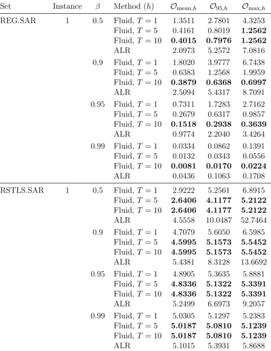
2.2 Objective value results (in %) for infinite horizon experiment, 𝑀 = 5,
𝑛 = 4, for instance 1 of sets REG.SAR and RSTLS.SAR. In each instance, value of 𝛽 and metric, the best value is indicated in bold. . 62
2.3 Objective value results (in %) for infinite horizon experiment, 𝑀 = 5,
𝑛 = 4, for instance 1 of sets RSTLS.SBR and RSTLS.DET.SBR. In each instance, value of 𝛽 and metric, the best value is indicated in bold. 63
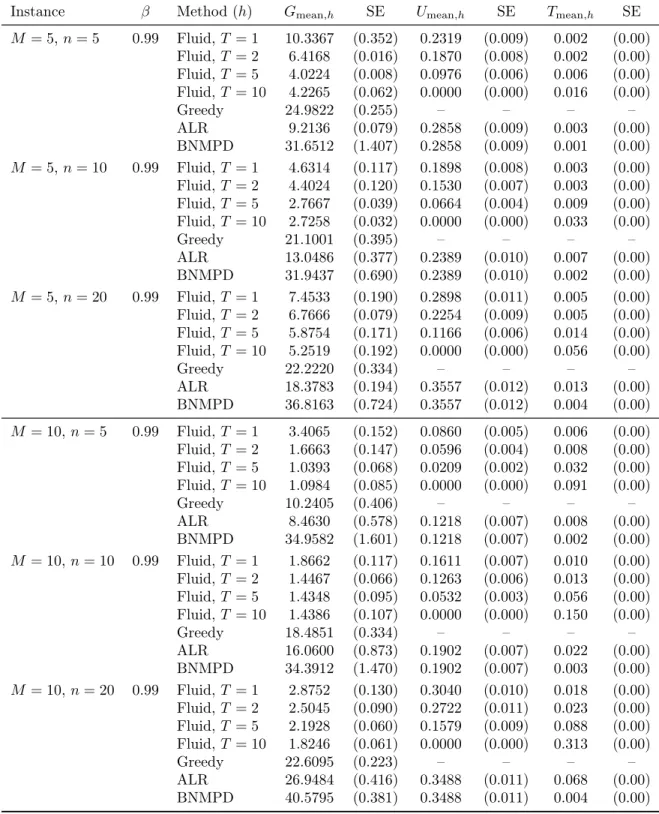
2.4 Large scale policy performance and runtime simulation results for 𝑀 ∈ {5, 10}, 𝑛 ∈ {5, 10, 20} RSTLS.DET.SBR instances. (SE indicates standard error.) . . . 66
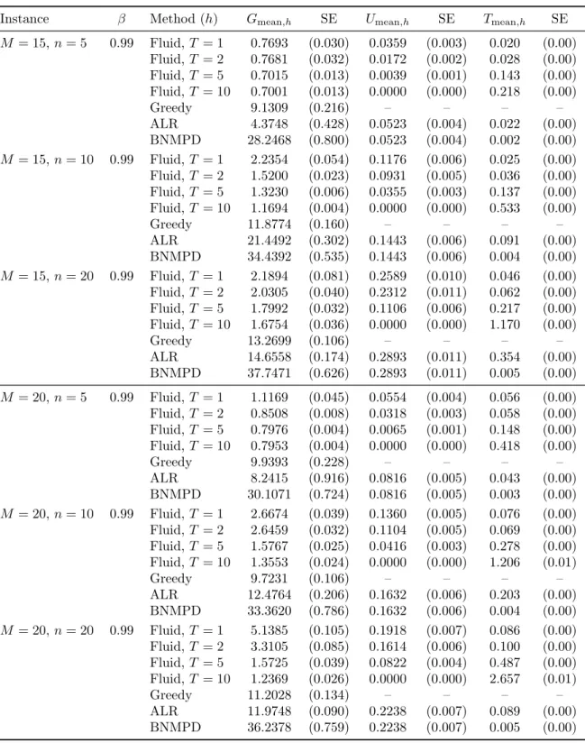
2.5 Large scale policy performance and runtime simulation results for 𝛽 = 0.99, 𝑀 ∈ {15, 20}, 𝑛 ∈ {5, 10, 20} RSTLS.DET.SBR instances. (SE
indicates standard error.) . . . 67
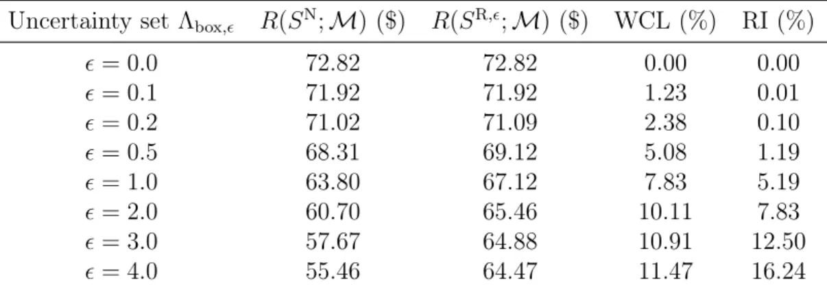
3.1 Worst-case loss of nominal solution and relative improvement of robust
solution over nominal solution for varying values of 𝜖. . . 96
3.2 Comparison of nominal and worst-case revenues for LCMNL model
under bootstrapping for 𝐾 ∈ {1, . . . , 10}. . . 97
3.3 Comparison of solutions under nominal HB models 𝑚𝑃 𝑜𝑖𝑛𝑡𝐸𝑠𝑡and 𝑚𝑃 𝑜𝑠𝑡𝐸𝑥𝑝 to robust solution under uncertainty set ℳ formed by posterior
3.4 Comparison of nominal and worst-case revenues of product lines 𝑆N,3, . . . , 𝑆N,12. 105
3.5 Performance of nominal and robust product lines under the different
models in ℳ as well as the worst-case model. . . 106
4.1 Results of tractability experiment. . . 133
4.2 Results of constrained optimization comparison. . . 137
4.3 Results of estimation procedure. . . 140
4.4 Results of estimation procedure as available data varies. . . 141
4.5 Results of estimation procedure as training MAE tolerance decreases. Results correspond to MMNL(5.0, 10) instances with 𝑛 = 30 products and 𝑀 = 20 training assortments. . . 142
4.6 Results of revenue prediction comparison for 𝑛 = 20 instances with 𝑀 = 20 training assortments. . . 144
4.7 Results of revenue prediction comparison between CG and MNL ap-proaches for 𝑛 = 20 instances with 𝐿 = 100.0, 𝑇 ∈ {5, 10}, as number of training assortments 𝑀 varies. . . 145
4.8 Results of combining the estimation and optimization procedures over a wide range of MMNL models. . . 148
4.9 Results of combining the estimation and optimization procedures as the amount of available data (the number of training assortments 𝑀 ) varies. . . 149
4.10 Results of combining the estimation and optimization procedures as training MAE tolerance varies. Results correspond to MMNL(5.0,10) instances with 𝑛 = 30 products and 𝑀 = 20 training assortments. . 150
4.11 Results of comparison of combined estimation-optimization approaches for 𝑛 = 20, MMNL(·, ·) instances. . . 152
4.12 Results of optimality gap comparison between MNL and CG+MIO approaches as number of training assortments 𝑀 varies, for 𝑛 = 20, MMNL instances with 𝐿 = 100.0 and 𝑇 ∈ {5, 10}. . . 153
5.1 Transaction data in example data set. . . 164 5.2 Results for 𝑛 = 10, 𝑀 = 5. (“Rev” indicates the out-of-sample revenue;
Chapter 1
Introduction
Modern business decisions exhibit an unprecedented level of complexity. Consider the following examples:
∙ Given a set of projects evolving stochastically, how should we dynamically al-locate our firm’s resources to these projects to maximize the long term benefit
to the firm?
∙ What variations of a new product should we offer to a customer population? ∙ How should we modify our product offerings to maximize revenues given
aggre-gated transaction data from a collection of customers?
∙ In an online retail setting, how do we leverage information about our customers to tailor our product offerings to each individual customer?
These decisions, and many other decisions like these ones, are extremely complex. Often, the system that provides the context for our decision is one that is
high-dimensional; that exhibits known, stochastic dynamics or otherwise, unknown dy-namics that lead to uncertainty in our decision; and ones that evolve over multiple
stages in time, requiring us to make not a single, one-shot decision, but a sequence of decisions. Such decisions exceed human decision making ability; managerial intuition
At the same time, businesses have increasing access to data and models that allow them to understand the effects of different decisions. For example, in the case
of product line decisions, firms increasingly rely on a technique known as conjoint analysis to survey customers, which involves asking representative customers to choose
from hypothetical products. Using this data on their choices, the firm can then build models to predict how customers will choose from hypothetical product offerings.
However, despite this increasing access to data and models, firms lack the
capa-bility to bridge the chasm between data/models and effective decisions. This is what the burgeoning field of analytics is concerned: how to transform data and predictive
models into decisions that create value.
This thesis is concerned with developing new analytics methods for making
com-plex decisions in the presence of either data or models that describe the system. These methods are largely based on modern optimization, more specifically, linear,
mixed-integer and robust optimization. In what follows, we provide a high-level overview of each chapter of the thesis. A more extensive discussion of the contributions and the
relevant literature can be found at the beginning of each chapter.
1.1
Decomposable Markov decision processes: a fluid
optimization approach
In Chapter 2, we consider the problem of solving decomposable Markov decision processes (MDPs). Decomposable MDPs are problems where the stochastic system
can be decomposed into multiple individual components. Although such MDPs arise naturally in many practical applications, they are often difficult to solve exactly
due to the enormous size of the state space of the complete system, which grows exponentially with the number of components.
In this chapter, we propose an approximate solution approach to decomposable MDPs that is based on re-solving a fluid linear optimization formulation of the
modeling transition behavior at the level of the individual components rather than the complete system. We prove that our fluid formulation provides a tighter bound on
the optimal value function than three state-of-the-art formulations: the approximate linear optimization formulation, the classical Lagrangian relaxation formulation and a
novel, alternate Lagrangian relaxation that is based on relaxing an action consistency constraint. We provide a numerical demonstration of the effectiveness of the approach
in the area of multiarmed bandit problems, where we show that our approach provides near optimal performance and outperforms state-of-the-art algorithms.
1.2
Robust product line design
In Chapter 3, we consider the problem of designing product lines that are immunized to uncertainty in customer choice behavior. The majority of approaches to product
line design that have been proposed by marketing scientists assume that the under-lying choice model that describes how the customer population will respond to a new
product line is known precisely. In reality, however, marketers do not precisely know how the customer population will respond and can only obtain an estimate of the
choice model from limited conjoint data.
In this chapter, we propose a new type of optimization approach for product line design under uncertainty. Our approach is based on the paradigm of robust
optimization where, rather than optimizing the expected revenue with respect to a single model, one optimizes the worst-case expected revenue with respect to an
uncertainty set of models. This framework allows us to account for both parameter uncertainty, when we may be confident about the type of model structure but not
about the values of the parameters, and structural uncertainty, when we may not even be confident about the right model structure to use to describe the customer
population.
Through computational experiments with a real conjoint data set, we demonstrate the benefits of our approach in addressing parameter and structural uncertainty. With
ac-counting for parameter uncertainty are fragile and can experience worst-case revenue losses as high as 23%, and that the robust product line can significantly outperform
the nominal product line in the worst-case, with relative improvements of up to 14%. With regard to structural uncertainty, we similarly show that product lines that are
designed for a single model structure can be highly suboptimal under other structures (worst-case losses of up to 37%), while a product line that optimizes against the worst
of a set of structurally distinct models can outperform single-model product lines by as much as 55% in the worst-case and can guarantee good aggregate performance
over structurally distinct models.
1.3
Data-driven assortment optimization
In Chapter 4, we consider the problem of assortment optimization using historical
transaction data from previous assortments. Assortment optimization refers to the problem of selecting a set of products to offer to a group of customers so as to
maximize the revenue that is realized when customers make purchases according to their preferences. Assortment optimization is essential to a wide variety of application
domains that includes retail, online advertising and social security; however, it is challenging in practice because one typically has limited data on customer choices on
which to base the decision.
In this chapter, we present a two-step approach to making effective assortment decisions from transaction data. In the first step, we use the data to estimate a generic
ranking-based model of choice that is able to represent any choice model based on random utility maximization. In the second step, using the estimated model, we find
the optimal assortment by solving a mixed-integer optimization (MIO) problem that is scalable and that is flexible, in that it can easily accommodate constraints.
We show through computational experiments with synthetic data that (1) our
MIO model is practically tractable and can be solved to full optimality for large numbers of products in operationally feasible times; (2) our MIO model is able to
esti-mation procedure is computationally efficient and produces accurate out-of-sample predictions of the true choice probabilities; and (4) by combining our estimation and
optimization procedures, we are able to find assortments that achieve near-optimal revenues that outperform alternative parametric and non-parametric approaches.
1.4
Personalized assortment planning via recursive
partitioning
In Chapter 5, we consider the problem of making personalized assortment decisions using data. Previously, in Chapter 4, we considered the problem of how to make an
assortment decision using historical data that only focuses on previous assortments and previous purchases, and does not assume that there is data about the customers
who make those purchase decisions. In an increasing number of real-world assortment contexts, we have access to information about a customer. For example, in an online
retail setting, we know information about the user browsing through the product offerings, such as their location (through their ZIP code for example), age, gender and
many other attributes. Given this information, how can we leverage this information to make a more effective assortment decision for each individual customer?
In this chapter, we present an approach for using auxiliary customer data to make better assortment decisions. The approach is based on building a predictive
model using recursive partitioning: the customers represented in the transactions are iteratively divided up according to their attributes, and the end result is a tree
repre-sentation of the customers, where each leaf corresponds to a collection of customers that share similar attributes and whose choice behavior is sufficiently homogeneous.
In a way, this tree can be thought of as a segmentation of the customers.
Using synthetic data, we compare our partitioning-based approach to a uniform
approach, which offers the same assortment to all customers and ignores the cus-tomer attribute data, and to a “perfect foresight” approach, which knows the ground
ap-proach leads to out-of-sample revenues that improve on the uniform apap-proach, and are moderately close to revenues obtained with perfect foresight.
Chapter 2
Decomposable Markov decision
processes: a fluid optimization
approach
2.1
Introduction
Many real world problems involving the control of a stochastic system can be modeled as Markov decision processes (MDPs). In a typical MDP, the system begins in a
certain state s in some state space 𝒮. The decision maker selects an action 𝑎 from some action space 𝒜. The system then transitions randomly to a new state s′ with probability 𝑝𝑎(s, s′) and the decision maker garners some reward 𝑔𝑎(s). Once the system is in this new state s′, the decision maker once again selects a new action, leading to additional reward and causing the system to transition again. In the most basic form of the problem, the decision maker needs to make decisions over an
infinite horizon, and the rewards accrued over this infinite horizon are discounted in time according to a discount factor 𝛽 ∈ (0, 1). The goal of the decision maker, then,
the expected total discounted reward E [︃ ∞ ∑︁ 𝑡=1 𝛽𝑡−1𝑔𝜋(s(𝑡))(s(𝑡)) ]︃ ,
where s(𝑡) is the random variable representing the state at time 𝑡, when the system is
operated according to policy 𝜋. In other types of problems, the decision maker may only be making decisions over a finite time horizon; in those problems, the policy
prescribing the action to take may not only depend on the state, but also on the time at which the decision is being made.
Although problems that are represented in this form can in principle be solved
ex-actly with dynamic programming, this is often practically impossible. Exact methods based on dynamic programming require one to compute the optimal value function
𝐽*, which maps states in the state space 𝒮 to the optimal expected discounted reward when the system starts in that state. For many problems of practical interest, the
state space 𝒮 is so large that operating on, or even storing the value function 𝐽*, becomes computationally infeasible. This is what is often referred to in the dynamic
programming and MDP literature as the curse of dimensionality [8].
Where does the curse of dimensionality come from? That is, why is it that practi-cal MDPs often have prohibitively large state spaces? For many practipracti-cal problems,
the system that is being modeled is often not a single, atomic system, but rather con-sists of a collection of smaller sub-systems or components. Mathematically, consider
a system consisting of 𝑀 components, where each component 𝑚 ∈ {1, . . . , 𝑀 } is endowed with a state 𝑠𝑚 from an ambient state space 𝒮𝑚. To represent the complete system, we must represent the state s as an 𝑀 -tuple of the component states, i.e., s = (𝑠1, . . . , 𝑠𝑀), and as a result, the state space of the complete system becomes the Cartesian product of the component state spaces, i.e., 𝒮 = 𝒮1 × · · · × 𝒮𝑀. As the number of components 𝑀 grows, the size of the state space of the complete system
grows in an exponential fashion.
At the same time, the data of such systems are often not presented to us in
candidate action in 𝒜 may be naturally expressed in terms of individual components or small combinations (e.g., pairs) of components. Similarly, the reward structure of
the problem does not need to be specified in terms of the complete system state, but can be specified in terms of the component states. In the remainder of the chapter,
we will refer to MDPs where the probabilistic dynamics and reward structure can be expressed in terms of the component states as decomposable MDPs.
Many practically relevant MDPs can be modeled as decomposable MDPs. One
major class of MDPs that falls into the decomposable MDP framework is the class of multiarmed bandit problems. In the multiarmed bandit problem, the decision maker
is presented with 𝑀 machines (“bandits”), where each bandit 𝑚 is initially in some state 𝑠𝑚 from its state space 𝒮𝑚. At each point in time, one of the bandits may be activated, in which case the chosen bandit changes state probabilistically and the decision maker earns some reward. The problem is then to decide, at each point in
time, given the state of all of the bandits, which bandit to activate, so as to maximize the total expected long term reward. In the basic form of the problem – the regular
multiarmed bandit problem – when a bandit 𝑚 is activated, the inactive bandits do not change state. In the restless bandit problem, the inactive bandits can also change
state passively and the decision maker may earn a passive reward from bandits that are not activated. The multiarmed bandit, by its definition, is a decomposable MDP:
the state space of the ensemble of bandits is the product of the state spaces of the individual bandits, and the probability transition structure is specified at the level of
each bandit.
In this chapter, we propose a new fluid optimization approach for approximately
solving decomposable MDPs. The centerpiece of our approach is a linear optimization (LO) model in which, in its most basic form, the decision variables represent the
marginal probabilities of each individual component being in each of its possible states and the action taken at a particular time, and the main constraints are conservation
constraints that govern how these marginal probabilities “flow” from component states at time 𝑡 to new states at 𝑡 + 1 under different action (hence the name fluid ). The
controlled optimally. The formulation achieves this in a tractable way by exploiting the decomposable nature of the problem: rather than modeling the precise transition
behavior of the system at the level of tuples of component states, it models the macroscopic transitions of the system at the level of the individual components and
their states. The optimal solution of the formulation, when it includes constraints that model the complete system starting in a certain state, can be used to derive an
action for the state. In this way, the formulation leads naturally to a simple heuristic for solving the MDP.
Our contributions are as follows:
1. We propose a novel LO formulation for approximately modeling decomposable MDPs and an associated heuristic for solving the MDP. The formulation is
tractable since the number of variables scales linearly with the number of indi-vidual components, as opposed to the exponential scaling that is characteristic
of dynamic programming. We show that this formulation provides an upper bound on the optimal value of the MDP and provide idealized conditions under
which our fluid formulation-based heuristic is optimal. We discuss how this basic, “first-order” formulation that models individual components can be
ex-tended to “higher-order” formulations that model combinations of components (e.g., a second-order formulation that models transitions of pairs of
compo-nents). We also discuss how the basic formulation can be extended to address finite horizon, time-dependent problems.
2. We theoretically compare our fluid formulation to three alternative proposals.
In particular, we show that a finite version of our formulation that models the evolution of the system over a horizon of 𝑇 periods provides provably tighter
bounds on the optimal value function than three state-of-the-art formulations: the approximate linear optimization (ALO) formulation of [38], the classical
Lagrangian relaxation (CLR) formulation of [2] and an alternate Lagrangian relaxation (ALR) that involves relaxing an action consistency constraint. The
to the ALO and is of independent interest. Moreover, the fluid bound is non-increasing with the time horizon 𝑇 . Letting 𝐽*(s) denote the optimal value function at the state s, 𝑍𝑇*(s) denote the objective value of the fluid formulation with horizon 𝑇 at s, and 𝑍𝐴𝐿𝑂* (s), 𝑍𝐴𝐿𝑅* (s),and 𝑍𝐶𝐿𝑅* (s) denote the objective values of the ALO, ALR and CLR formulations at s, respectively, our results can be summarized in the following statement, which holds for any 𝑇 ∈ {1, 2, . . . }:
𝐽*(s) ≤ 𝑍𝑇*(s) ≤ . . . ≤ 𝑍2*(s) ≤ 𝑍1*(s) ≤ 𝑍𝐴𝐿𝑂* (s) = 𝑍𝐴𝐿𝑅* (s) ≤ 𝑍𝐶𝐿𝑅* (s).
In this way, our work contributes to the overall understanding of the fluid ap-proach and all previous proposals in a unified framework.
3. We demonstrate the effectiveness of our approach computationally on
multi-armed bandit problems. We consider regular bandit problems (inactive bandits
do not change state) and restless bandit problems (inactive bandits may change state). We show that bounds from our approach can be substantially tighter
than those from state-of-the-art approaches, and that the performance of our fluid policy is near-optimal and outperforms policies from state-of-the-art
ap-proaches.
The rest of this chapter is organized as follows. In Section 2.2, we review the extant body of research related to this chapter. In Section 2.3, we define the
decom-posable MDP and present our infinite LO fluid formulation. We prove a number of properties of this formulation, and motivated by the properties of this infinite LO
for-mulation, we present a heuristic policy for generating actions at each decision epoch based on a finite version of this formulation. In Section 2.4, we compare the finite
fluid formulation to the ALO formulation of [38], the classical Lagrangian relaxation approach of [2] and the alternate Lagrangian relaxation. In Section 2.5, we apply our
framework to the multiarmed bandit problem and provide computational evidence for the strength of our approach in this class of problems. Finally, in Section 2.6, we
2.2
Literature review
Markov decision processes have a long history, tracing back to the work of [7] in the
1950s. The importance and significance of this area in the field of operations research is underscored both by the number of research papers that have been written in this
area, as well as the numerous books written on the subject [60, 59, 75, 12].
While MDPs can be solved exactly through methods such as value iteration, policy iteration and the LO approach (see, e.g., [75]), these approaches become intractable
in high-dimensional problems. As a result, much research has been conducted in the area of approximate dynamic programming (ADP). The interested reader is referred
to [94] for a brief overview, and to [13] and [74] for more comprehensive treatments of the topic. The goal of ADP is to find an approximation to the true value function.
By then applying the policy that is greedy with respect to this approximate value function, one hopes to achieve performance that is close to that of the true optimal
policy.
Within the ADP literature, our work is most closely related to the approximate linear optimization (ALO) approach of [38] and the Lagrangian relaxation approach
of [2]. In the ALO approach to ADP, one approximates the value function as the weighted sum of a collection of basis functions, and solves the LO formulation of the
MDP with this approximate value function in place of the true value function. By doing so, the number of variables in the problem is significantly reduced, leading to
a more tractable problem. In many applications, one can exploit the decomposable nature of the problem in selecting a basis function architecture: for example, in [38]
the approach is applied to a queueing control example, where the value function is approximated as a linear combination of all polynomials up to degree 2 of the
indi-vidual queue lengths of the system. On the other hand, [58] and [2] study MDPs where the problem can be viewed as a collection of subproblems, and the action that
can be taken in each subproblem is constrained by a global linking constraint that couples the subproblems together. By dualizing the linking constraint, the complete
is significantly simpler than the exact LO model of the MDP. By solving this opti-mization problem, one obtains an upper bound on the optimal value at a given state
and a value function approximation.
Our fluid approach is closely related to the Lagrangian relaxation approach and builds on it in two important ways. First, we delineate two different types of
La-grangian relaxations: the “classical” LaLa-grangian relaxation, where the action space is implicitly defined by a coupling constraint, and a novel, “alternate” Lagrangian
relaxation where the components are coupled by an “action consistency” constraint (the action taken in each component must be the same). Our formulation is not
related to the former classical formulation, but to the latter alternate formulation. This alternate Lagrangian relaxation is significant because it extends the scope of the
Lagrangian relaxation approach to problems that do not have a decomposable system action space. Furthermore, it turns out that this alternate Lagrangian relaxation is
actually equivalent to the ALO: the two models lead to the same bound on the true optimal value function and the same value function approximation (Theorem 2). In
contrast, for the classical Lagrangian relaxation, one can only show that the ALO bound is at least as tight [2] and one can find simple examples where the Lagrangian
bound can be significantly worse than the ALO bound.
The second way in which our approach builds on the Lagrangian relaxation
ap-proach is through its view of time. Our formulation first models the state of each component separately at each decision epoch over a finite horizon before aggregating
them over the remaining infinite horizon, whereas the formulation of [2] aggregates them over the entire infinite horizon. While this may appear to be a superficial
dif-ference, it turns out to be rather significant because it allows us to prove that the fluid bound is at least as tight as the classical and alternate Lagrangian relaxation
bounds (parts (a) and (c) of Theorem 3). As we will see in Section 2.5, the difference in the bounds and the associated performance can be considerable.
With regard to the ALO, the ALO and our fluid model differ in tractability. In particular, the size (number of variables and number of constraints) of our fluid model
while the number of variables may scale linearly in the number of components, the number of constraints still scales linearly with the number of system states, as in the
exact LO model of the MDP. This necessitates the use of additional techniques to solve the problem, such as constraint sampling [39]. Moreover, as stated above, it
turns out that when one uses a component-wise approximation architecture for the ALO, it is equivalent to the alternate Lagrangian relaxation formulation described
above. Due to this equivalence, we are able to assert that our fluid model leads to better bounds than the ALO, and through our numerical results, that our fluid
approach leads to better performance than the ALO approach.
Outside of ADP, many approximate approaches to stochastic control problems also exploit decomposability. One salient example of this is the performance region
approach to stochastic scheduling. In this approach, one considers a vector of per-formance measures of the complete system (for an overview, [14]). Using the
proba-bilistic dynamics of the system, one can then derive conservation laws that constrain the values this vector of performance measures may take. The resulting set is the
performance region of the system, over which one can solve an optimization problem to find the best vector of performance measures. It turns out that typically this vector
of performance measures is achieved by simple policies or a randomization of simple policies. This approach was introduced by [35] for multi-class scheduling in a
single-server 𝑀/𝑀/1 queue and later extended by [45] and [88] to more general queueing systems. [18] unified this framework and extended it beyond queueing control
prob-lems to such probprob-lems as the multiarmed bandit problem and branching bandits. [19] later considered a performance region formulation for the restless bandit problem and
used it to derive a high quality heuristic for the restless bandit problem.
Our approach has some conceptual similarities to the performance region approach
in the sense that one defines decision variables related to the proportion of time that components of the system are in certain states, imposes constraints that conserve
these proportions with each transition and optimizes an objective over the resulting feasible set. In spite of these commonalities, there are a number of key differences.
system, possess attractive computational and theoretical properties. For example, for systems that satisfy generalized conservation laws, the performance region is an
extended polymatroid or contra-polymatroid and so a linear function can be optimized rapidly using a greedy algorithm, and the extreme points of the performance region
correspond to deterministic priority rules [18]. In contrast, our formulation does not appear to possess such special computational structure and, as we discuss in
Section 2.3.3, optimal solutions of our fluid formulation may in general not be achieved by any policy, let alone a specific class of policies. At the same time, many extant
performance region approaches are fragile, in that they exploit non-trivial properties of the underlying stochastic system and thus cannot be immediately extended to
even simple generalizations. An example of this is the formulation of the multiarmed bandit problem in [18], which exploits specific conservation properties of the regular
multiarmed bandit problem and cannot be extended to restless bandits, necessitating the authors’ exploration of an alternate approach in [19]. In contrast, our formulation
is insensitive to these types of differences; it does not use any structure of the problem beyond the transition probabilities of individual components or groups of components.
Within the performance region literature, our fluid formulation of the restless
ban-dit problem is similar to the performance region model of [19]. This model is actually equivalent to both the classical and the alternate Lagrangian relaxation formulations
(Propositions 8 and 9). As a result, our comparison of the fluid formulation with the Lagrangian relaxation formulations allows us to assert that our approach leads to
tighter state-wise bounds than the performance region formulation. Moreover, as we will see in Section 2.5.5, our fluid approach significantly outperforms the associated
primal dual heuristic of [19].
The first fluid formulation that we will propose in Section 2.3.2 is a countably
infinite LO (CILO) problem. There exists a rich literature on this class of problems (see, e.g., [5]). Within this area, the work of [50] and [68] directly studies MDPs;
however, both of these papers specifically study nonstationary problems and do not additionally consider decomposability. Although we do not explore the application of
an interesting direction for future research.
Lastly, the alternate Lagrangian relaxation we will develop in Section 2.4 arises
by relaxing a certain type of action consistency constraint that requires that the action taken in any two components be equivalent. This bears some resemblance to
the technique of “variable splitting” or “operator splitting” that is used in continuous optimization (see, for example, [27, 52] and the references therein). The exploration of
the connections of the alternate Lagrangian relaxation to splitting-based formulations is an interesting direction for future research.
2.3
Methodology
We begin in Section 2.3.1 by defining a general decomposable, infinite horizon MDP.
We then present an infinite LO formulation that is related to this MDP in Sec-tion 2.3.2. In SecSec-tion 2.3.3, we prove some interesting properties of the formulaSec-tion,
and motivated by one of these properties, propose a solvable finite LO formulation and an associated heuristic in Section 2.3.4. The proofs of all theoretical results are
provided in Appendix A.1.
2.3.1
Problem definition
In this section, we define the decomposable MDP for which we will subsequently
develop our fluid approach.
Let 𝒮 be the state space of the complete system, and assume that the complete system state decomposes into 𝑀 components, so that the complete system state space
can be written as 𝒮 = 𝒮1× · · · × 𝒮𝑀. Let 𝒜 be a finite action space, and assume that any action in 𝒜 can be taken at any state in 𝒮. We make this assumption
for simplicity; our approach can be extended to accommodate component-dependent constraints that restrict which actions can be action when specific components enter
specific states (for example, an action 𝑎 cannot be taken when component 𝑚 is in state 𝑘). Let s(𝑡) be the random variable that represents the state of the complete
that s(𝑡) = (𝑠1(𝑡), . . . , 𝑠𝑀(𝑡)). Let 𝜋 : {1, 2, . . . } × 𝒮 → 𝒜 be the policy under which the system is operating, which maps a state s(𝑡) at time 𝑡 to an action 𝜋(𝑡, s(𝑡)) in 𝒜. Let 𝑝𝑎(s, ¯s) be the probability of the complete system transitioning from state s to state ¯s in one step when action 𝑎 ∈ 𝒜 is taken, i.e.,
𝑝𝑎(s, ¯s) = P (s(𝑡 + 1) = ¯s s(𝑡) = s, 𝜋(𝑡, s(𝑡)) = 𝑎)
for all 𝑡 ∈ {1, 2, . . . }. Let 𝑝𝑚𝑘𝑗𝑎 denote the probability of component 𝑚 transitioning from state 𝑘 to state 𝑗 in one step when action 𝑎 ∈ 𝒜 is taken, i.e.,
𝑝𝑚𝑘𝑗𝑎= P(𝑠𝑚(𝑡 + 1) = 𝑗 𝑠𝑚(𝑡) = 𝑘, 𝜋(𝑡, s(𝑡)) = 𝑎),
for all 𝑡 ∈ {1, 2, . . . }. We assume that the components are independent, so that
𝑝𝑎(s, ¯s) can be written compactly as
𝑝𝑎(s, ¯s) = 𝑀 ∏︁ 𝑚=1
𝑝𝑚𝑠𝑚𝑠¯𝑚𝑎.
Let 𝑔𝑎(s) be the reward associated with taking action 𝑎 when the system is in state s, and assume that it is additive in the components, that is, it can be written
as 𝑔𝑎(s) = 𝑀 ∑︁ 𝑚=1 𝑔𝑚𝑠𝑚𝑎, where 𝑔𝑚
𝑘𝑎is the reward associated with taking action 𝑎 when component 𝑚 is in state 𝑘. Assume that the system starts in state s = (𝑠1, . . . , 𝑠𝑀). The problem is then to find a policy 𝜋 that maximizes the expected total discounted reward:
max 𝜋 E [︃ ∞ ∑︁ 𝑡=1 𝑀 ∑︁ 𝑚=1 𝛽𝑡−1𝑔𝑠𝑚𝑚(𝑡),𝜋(𝑡,s(𝑡)) s(1) = s ]︃ . (2.1)
2.3.2
Fluid linear optimization formulation
We now consider a fluid formulation of problem (2.1). We begin by defining, for
component 𝑚 ∈ {1, . . . , 𝑀 } is in state 𝑘 ∈ 𝒮𝑚 and action 𝑎 ∈ 𝒜 is taken at time 𝑡. For every 𝑡 ∈ {1, 2, 3, . . . }, we also define the decision variable 𝐴𝑎(𝑡) to be the proportion of time that action 𝑎 ∈ 𝒜 is taken at time 𝑡. As stated in Section 2.3.1, our data are the discount factor 𝛽, the reward 𝑔𝑚
𝑘𝑎 (the reward accrued by the decision maker when component 𝑚 is in state 𝑘 and action 𝑎 is taken) and the transition probability 𝑝𝑚
𝑘𝑗𝑎(the probability that component 𝑚 transitions from state 𝑘 to state 𝑗 in one step when action 𝑎 is taken).
Finally, we assume that the system starts deterministically in a state s ∈ 𝒮. For
convenience, we will define 𝛼𝑚𝑘(s) as
𝛼𝑚𝑘(s) = ⎧ ⎨ ⎩ 1, if 𝑠𝑚 = 𝑘, 0, otherwise.
The fluid problem for initial state s can now be formulated as follows:
maximize x,A ∞ ∑︁ 𝑡=1 𝑀 ∑︁ 𝑚=1 ∑︁ 𝑘∈𝒮𝑚 ∑︁ 𝑎∈𝒜 𝛽𝑡−1· 𝑔𝑘𝑎𝑚 · 𝑥𝑚𝑘𝑎(𝑡) (2.2a) subject to ∑︁ 𝑎∈𝒜 𝑥𝑚𝑗𝑎(𝑡) = ∑︁ 𝑘∈𝒮𝑚 ∑︁ ˜ 𝑎∈𝒜 𝑝𝑚𝑘𝑗˜𝑎𝑥𝑚𝑘˜𝑎(𝑡 − 1), ∀ 𝑚 ∈ {1, . . . , 𝑀 }, 𝑡 ∈ {2, 3, . . . }, 𝑗 ∈ 𝒮𝑚, (2.2b) ∑︁ 𝑘∈𝒮𝑚 𝑥𝑚𝑘𝑎(𝑡) = 𝐴𝑎(𝑡), ∀ 𝑚 ∈ {1, . . . , 𝑀 }, 𝑎 ∈ 𝒜, 𝑡 ∈ {1, 2, . . . }, (2.2c) ∑︁ 𝑎∈𝒜 𝑥𝑚𝑘𝑎(1) = 𝛼𝑚𝑘(s), ∀ 𝑚 ∈ {1, . . . , 𝑀 }, 𝑘 ∈ 𝒮𝑚, (2.2d) 𝑥𝑚𝑘𝑎(𝑡) ≥ 0, ∀ 𝑚 ∈ {1, . . . , 𝑀 }, 𝑎 ∈ 𝒜, 𝑘 ∈ 𝒮𝑚, 𝑡 ∈ {1, 2, . . . }, (2.2e) 𝐴𝑎(𝑡) ≥ 0, ∀ 𝑎 ∈ 𝒜, 𝑡 ∈ {1, 2, . . . }. (2.2f)
Constraint (2.2b) ensures that probability is conserved from time 𝑡 − 1 to time 𝑡: the left hand side represents the proportion of time that component 𝑚 is in state 𝑗
same proportion, only in terms of the 𝑥𝑚𝑘˜𝑎(𝑡 − 1) variables, which correspond to time 𝑡 − 1. Constraint (2.2c) ensures that, for each component, the proportion of time
that action 𝑎 is taken in terms of the 𝑥𝑚𝑘𝑎(𝑡) variables is equal to 𝐴𝑎(𝑡) (which is precisely defined as the proportion of time that action 𝑎 is taken at time 𝑡). Thus,
the actions 𝑎 ∈ 𝒜 connect the variables corresponding to the different components. Constraint (2.2d) ensures that the initial frequency with which each component 𝑚 is
in a state 𝑘 is exactly 𝛼𝑚𝑘(s). The remaining two constraints (2.2e) and (2.2f) ensure that all of the decision variables are nonnegative, as they represent proportions. Given
the definition of 𝑥𝑚𝑘𝑎(𝑡) as the proportion of time that component 𝑚 is in state 𝑘 at time 𝑡 and action 𝑎 is taken at time 𝑡, the objective can therefore be interpreted as
the expected discounted long term reward.
Note that constraints (2.2b) and (2.2d), together with the fact that∑︀
𝑗∈𝒮𝑚𝑝𝑚𝑘𝑗𝑎 = 1
for any 𝑚, 𝑘 and 𝑎, imply that ∑︀ 𝑘∈𝒮𝑚
∑︀ 𝑎∈𝒜𝑥
𝑚
𝑘𝑎(𝑡) = 1 for each 𝑚 and 𝑡. Together with constraint (2.2c), this also implies that ∑︀
𝑎∈𝒜𝐴𝑎(𝑡) = 1 for each 𝑡.
The following result, which follows by standard arguments in infinite dimensional linear optimization (see Section A.1.1 in Appendix A), establishes that the infinite
horizon problem (2.2) is well-defined.
Proposition 1 For each s ∈ 𝒮, problem (2.2) has an optimal solution.
2.3.3
Properties of the infinite fluid LO
We will now develop some theoretical properties of the fluid LO model. Let (x(s), A(s))
and 𝑍*(s) denote an optimal solution and the optimal objective value, respectively, to problem (2.2) corresponding to initial state s. Denote by 𝐽*(·) the optimal value function obtained using dynamic programming, that is,
𝐽*(s) = max 𝜋 E [︃ ∞ ∑︁ 𝑡=1 𝑀 ∑︁ 𝑚=1 𝛽𝑡−1𝑔𝑠𝑚𝑚(𝑡),𝜋(𝑡,s(𝑡)) s(1) = s ]︃
for every s ∈ 𝒮. We then have the following relationship between problem (2.2) and
Proposition 2 For every s ∈ 𝒮, 𝐽*(s) ≤ 𝑍*(s).
The idea behind the proof of Proposition 2, is that by using an optimal policy 𝜋*, it is possible to construct a feasible solution (x, A) to problem (2.2) whose objective value is the true optimal value 𝐽*(s). Unfortunately, the opposite inequality does not hold in general; see Appendix A.2 counterexample. Let us call the optimal solution (x(s), A(s)) achievable if there exists a (possibly non-deterministic and time-varying)
policy 𝜋 such that
𝑥𝑚𝑘𝑎(𝑡, s) = P(𝑠𝑚(𝑡) = 𝑘, 𝜋(𝑡, s(𝑡)) = 𝑎), ∀ 𝑚 ∈ {1, . . . , 𝑀 }, 𝑘 ∈ 𝒮𝑚, 𝑎 ∈ 𝒜, 𝑡 ∈ {1, 2, . . . },
𝐴𝑎(𝑡, s) = P(𝜋(𝑡, s(𝑡)) = 𝑎), ∀ 𝑎 ∈ 𝒜, 𝑡 ∈ {1, 2, . . . },
where s(𝑡) is the state of the complete system stochastic process at time 𝑡, operated according to 𝜋, starting from s (i.e., s(1) = s). (Note that we use 𝑥𝑚
𝑘𝑎(𝑡, s) and 𝐴𝑎(𝑡, s) to denote the optimal value of 𝑥𝑚𝑘𝑎(𝑡) and 𝐴𝑎(𝑡) in the solution (x(s), A(s)) that corresponds to initial state s.) Under the assumption of achievability, we have
the following result.
Proposition 3 Let s ∈ 𝒮. If (x(s), A(s)) is achievable, then 𝑍*(s) ≤ 𝐽*(s).
The proof is contained Section A.1.3 of Appendix A. The result follows since, under
the assumption of achievability, 𝑍*(s) is the total expected discounted reward of some policy, while 𝐽*(s) is the highest any such reward can be.
Under the assumptions of component independence and achievability, the fluid formulation allows us to construct an optimal policy.
Theorem 1 Suppose that for all s ∈ 𝒮, (x(s), A(s)) is achievable. Define the deter-ministic, stationary policy 𝜋 : 𝒮 → 𝒜 as
𝜋(s) = arg max
𝑎∈𝒜 𝐴𝑎(1, s).
Under these assumptions, the policy 𝜋 is an optimal policy, i.e., 𝜋 solves
The proof of the result (found in Section A.1.4 of Appendix A) follows by showing that any action 𝑎 such that 𝐴𝑎(1, s) > 0 is an action that is greedy with respect to the objective value 𝑍*(·) which, by combining Propositions 2 and 3, is equal to the optimal value function 𝐽*(·).
2.3.4
Fluid-based heuristic
Theorem 1 tells us that, assuming that for every initial state s the optimal solution of
problem (2.2) for initial state s is achievable, we immediately have an optimal policy by simply looking at the optimal values of the 𝐴 variables at the first period (𝑡 = 1).
Typically, however, the optimal solution of (2.2) will not be achievable. It nevertheless seems reasonable to expect that in many problems, the optimal solution (x(s), A(s))
may be close to being achievable for many states s, because (x(s), A(s)) still respects the transition behavior of the system at the level of individual components.
Con-sequently, the action arg max𝑎∈𝒜𝐴𝑎(1, s) should then be close to an optimal action for many states s. It is therefore reasonable to expect that, by selecting the action
𝑎 as arg max𝑎∈𝒜𝐴𝑎(1, s), one may often still be able to get good performance, even though the optimal solution of problem (2.2) may not be achievable.
Notwithstanding the question of achievability, applying this intuition in practice is not immediately possible. The reason for this is that problem (2.2) is an LO problem
with a countably infinite number of variables and constraints, and so cannot be solved using standard solvers. Towards the goal of developing a practical heuristic policy
for problem (2.1), we now consider an alternate, finite problem that can be viewed as an approximation to problem (2.2). This new formulation, presented below as
problem (2.3), requires the decision maker to specify a time horizon 𝑇 over which the evolution of the system will be modeled. For 𝑡 ∈ {1, . . . , 𝑇 }, the variables 𝑥𝑚
𝑘𝑎(𝑡) and 𝐴𝑎(𝑡) have the same meaning as in problem (2.3). To model the evolution of the system beyond 𝑡 = 𝑇 , we use the variable 𝑥𝑚
𝑘𝑎(𝑇 + 1) to represent the expected discounted long-run frequency with which component 𝑚 is in state 𝑘 and action 𝑎 is taken from 𝑡 = 𝑇 + 1 on. Similarly, we use 𝐴𝑎(𝑇 + 1) to represent the expected discounted frequency with which action 𝑎 is taken from 𝑡 = 𝑇 + 1 on.
With these definitions, the formulation corresponding to initial state s is presented below. maximize x,A 𝑇 +1 ∑︁ 𝑡=1 𝑀 ∑︁ 𝑚=1 ∑︁ 𝑘∈𝒮𝑚 ∑︁ 𝑎∈𝒜 𝛽𝑡−1· 𝑔𝑚 𝑘𝑎· 𝑥 𝑚 𝑘𝑎(𝑡) (2.3a) subject to ∑︁ 𝑎∈𝒜 𝑥𝑚𝑗𝑎(𝑡) = ∑︁ 𝑘∈𝒮𝑚 ∑︁ ˜ 𝑎∈𝒜 𝑝𝑚𝑘𝑗˜𝑎· 𝑥𝑚 𝑘˜𝑎(𝑡 − 1), ∀ 𝑚 ∈ {1, . . . , 𝑀 }, 𝑡 ∈ {2, . . . , 𝑇 }, 𝑗 ∈ 𝒮𝑚, (2.3b) ∑︁ 𝑎∈𝒜 𝑥𝑚𝑗𝑎(𝑇 + 1) = ∑︁ 𝑘∈𝒮𝑚 ∑︁ 𝑎∈𝒜 𝑝𝑚𝑘𝑗𝑎· 𝑥𝑚𝑘𝑎(𝑇 ) + 𝛽 · ∑︁ 𝑘∈𝒮𝑚 ∑︁ 𝑎∈𝒜 𝑝𝑚𝑘𝑗𝑎· 𝑥𝑚𝑘𝑎(𝑇 + 1), ∀ 𝑚 ∈ {1, . . . , 𝑀 }, 𝑗 ∈ 𝒮𝑚, (2.3c) ∑︁ 𝑘∈𝒮𝑚 𝑥𝑚𝑘𝑎(𝑡) = 𝐴𝑎(𝑡), ∀ 𝑚 ∈ {1, . . . , 𝑀 }, 𝑎 ∈ 𝒜, 𝑡 ∈ {1, . . . , 𝑇 + 1} (2.3d) ∑︁ 𝑎∈𝒜 𝑥𝑚𝑘𝑎(1) = 𝛼𝑚𝑘(s), ∀ 𝑚 ∈ {1, . . . , 𝑀 }, 𝑘 ∈ 𝒮𝑚, (2.3e) 𝑥𝑚𝑘𝑎(𝑡) ≥ 0, ∀ 𝑚 ∈ {1, . . . , 𝑀 }, 𝑎 ∈ 𝒜, 𝑘 ∈ 𝒮𝑚, 𝑡 ∈ {1, . . . , 𝑇 + 1}, (2.3f) 𝐴𝑎(𝑡) ≥ 0, ∀ 𝑎 ∈ 𝒜, 𝑡 ∈ {1, . . . , 𝑇 + 1}. (2.3g)
With regard to constraints, we retain the same conservation constraints that relate
the 𝑥𝑚𝑘𝑎variables at 𝑡−1 to 𝑡, the initial state constraint and the consistency constraints that relate the 𝑥𝑚
𝑘𝑎 and the 𝐴𝑎 variables at a time 𝑡, for 𝑡 ∈ {1, . . . , 𝑇 }. Beyond 𝑡 = 𝑇 , constraint (2.3c) models the long-run transition behavior of the system. This constraint can be interpreted as a conservation relation: the left hand side represents
the expected discounted number of times from 𝑇 + 1 on that we take an action out of component 𝑚 being in state 𝑗, while the right hand side represents the expected
discounted number of times that we enter state 𝑗 from 𝑇 + 1 on. More specifically, the first right-hand side term represents the expected number of times that we enter state
𝑗 at time 𝑇 + 1 (which is not discounted, since 𝑇 + 1 is the first period of the horizon {𝑇 + 1, 𝑇 + 2, 𝑇 + 3, . . . }) and the second term represents the expected discounted
number of times that we enter state 𝑗 from 𝑇 + 2 on. Note also that constraint (2.3d), which is the analog of constraint (2.2c), extends from 𝑡 = 1 to 𝑡 = 𝑇 +1, ensuring that
the 𝑥𝑚𝑘𝑎(𝑇 + 1) and the 𝐴𝑎(𝑇 + 1) variables are also consistent with each other. With regard to the objective, observe that rather than being an infinite sum from 𝑡 = 1,
the objective of problem (2.3) is a finite sum that extends from 𝑡 = 1 to 𝑡 = 𝑇 + 1. Let 𝑍𝑇*(s) denote the optimal value of problem (2.3). Problem (2.3), like prob-lem (2.2), provides an upper bound on the optimal value function at 𝐽*(s), and this bound improves with 𝑇 , as indicated by the following result.
Proposition 4 For each s ∈ 𝒮 and all 𝑇 ∈ {1, 2, . . . }:
(a) 𝑍𝑇*(s) ≥ 𝐽*(s); and
(b) 𝑍𝑇*(s) ≥ 𝑍𝑇 +1* (s).
The proof of part (a) of Proposition 4 follows along similar lines to Proposition 2,
while the proof of part (b) follows by showing that a solution to problem (2.3) with 𝑇 + 1 can be used to construct a feasible solution for problem (2.3) with 𝑇 that
achieves an objective value of 𝑍𝑇 +1* (s). The proof of this proposition can be found in Section A.1.5 of Appendix A. Part (a) of the proposition is useful because in passing
from the infinite to the finite formulation, we have not lost the useful property that the objective value provides an upper bound on the optimal value function. Part (b)
is important because it suggests a tradeoff in bound quality and computation: by increasing 𝑇 , the quality of the bound improves, but the size of the formulation (the
number of variables and constraints) increases. We will see later in Sections 2.5.4 and
2.5.5 that typically 𝑇 does not need to be very large to ensure strong bounds and performance.
With this formulation, our heuristic policy is then defined as Algorithm 1.
Before continuing, we comment on two important ways in which problem (2.3) can
be extended and one limitation of formulation (2.3). First of all, in problem (2.3), we formulated the decomposable MDP problem by defining decision variables that
Algorithm 1 Fluid LO heuristic for infinite horizon problem with known stationary probabilities.
Require: Parameter 𝑇 ; data p, g, 𝛽; current state s ∈ 𝒮.
Solve problem (2.3) corresponding to initial state s, horizon 𝑇 and data p, g, 𝛽 to obtain an optimal solution (x(s), A(s)).
Take action ˜𝑎, where ˜𝑎 = arg max𝑎∈𝒜𝐴𝑎(1, s).
with which a single component (component 𝑚) is in state 𝑘 and action 𝑎 is taken at
time 𝑡. As shown in Section 2.3.3, the resulting formulation provides an upper bound on the optimal expected discounted reward. We can improve on this by considering
higher-order fluid formulations, where rather than defining our decision variables to correspond to one component being in a state, we can define decision variables
cor-responding to combinations of components being in combinations of states, while a certain action is taken at a certain time. For example, a second-order formulation
would correspond to using decision variables that model how frequently pairs of com-ponents are in different pairs of states while an action is taken at each time. As the
order of the formulation increases, the objective value becomes an increasingly tighter bound on the optimal value, and it may be reasonable to expect better performance
from using Algorithm 1; however, the size of the formulation increases rapidly.
Second, problem (2.3) models an infinite horizon problem and Algorithm 1 is a heuristic for this problem. For finite horizon problems, we can apply our approach
as follows. Problem (2.3) can be modified by setting 𝑇 to the horizon of the actual problem and removing the terminal 𝑇 + 1 decision variables that model the long-run
evolution of the system. Then, if we are at state s at period 𝑡′, we restrict the fluid problem to {𝑡′, 𝑡′ + 1, . . . , 𝑇 } and use constraint (2.3e) to set the initial state at 𝑡′ to s. We then solve the problem to obtain the optimal solution (x(s), A(s)) and we take the action 𝑎 that maximizes 𝐴𝑎(𝑡, s). Note that if the transition probabilities change over time (i.e., rather than 𝑝𝑚𝑘𝑗𝑎 we have 𝑝𝑚𝑘𝑗𝑎(𝑡) for 𝑡 ∈ {1, . . . , 𝑇 − 1}), we may also modify constraint (2.3b) and replace 𝑝𝑚
𝑘𝑗𝑎 with 𝑝𝑚𝑘𝑗𝑎(𝑡), without changing the size or the nature of the resulting formulation.
Finally, we comment on one limitation to the fluid formulation (2.3).
the 𝑥𝑚𝑘𝑎(𝑡) and 𝐴𝑎(𝑡) variables are elements of the system action space 𝒜. For certain problems, the system action space 𝒜 may be small and problem (2.3) may be easy
to solve. For example, in a multiarmed bandit problem where exactly one bandit must be activated, |𝒜| = 𝑀 (one of the 𝑀 bandits); similarly, in an optimal stopping
problem, |𝒜| = 2 (stop or continue). For other problems, the action space of the problem may grow exponentially (e.g., a bandit problem where one may activate up
to 𝐾 of 𝑀 bandits). For such problems, the fluid formulation (2.3) will be harder to solve; we do not consider this regime here. The development of a scalable solution
method for large scale versions of problem (2.3) constitutes an interesting direction for future research.
2.4
Comparisons to other approaches
In this section, we compare our finite fluid formulation (2.3) against three
state-of-the-art formulations that can be used to solve decomposable MDPs. We begin by
stating these formulations: in Sections 2.4.1, 2.4.2 and 2.4.3, we present the ALO, classical Lagrangian relaxation and the alternate Lagrangian relaxation formulations,
respectively. Then, in Section 2.4.4 we state a key theoretical result that asserts that the finite fluid formulation (2.3) provides a provably tighter bound than all three
formulations. Finally, we conclude with a discussion of the sizes of the formulations in Section 2.4.5.
2.4.1
Approximate linear optimization
For the ALO formulation of [38], we approximate the value function using the same
functional form as in [2]: 𝐽𝐴𝐿𝑂(s) = 𝑀 ∑︁ 𝑚=1 𝐽𝑠𝑚𝑚, (2.4)