A multipole based Boundary Element Method for moving boundary problem in axisymmetric geometry

(1)

HAL Id: hal-00392329

https://hal.archives-ouvertes.fr/hal-00392329

Submitted on 13 Feb 2020

HAL is a multi-disciplinary open access

archive for the deposit and dissemination of sci-entific research documents, whether they are pub-lished or not. The documents may come from teaching and research institutions in France or abroad, or from public or private research centers.

L’archive ouverte pluridisciplinaire HAL, est destinée au dépôt et à la diffusion de documents scientifiques de niveau recherche, publiés ou non, émanant des établissements d’enseignement et de recherche français ou étrangers, des laboratoires publics ou privés.

Distributed under a Creative Commons Attribution| 4.0 International License

moving boundary problem in axisymmetric geometry

Jitendra Singh, Alain Glière, Jean-Luc Achard

To cite this version:

Jitendra Singh, Alain Glière, Jean-Luc Achard. A multipole based Boundary Element Method

for moving boundary problem in axisymmetric geometry. 30 th International Conference on

Boundary Elements and other Mesh Reduction Methods., Jul 2009, Maribor, Slovenia. pp.43-54, �10.2495/BE080051�. �hal-00392329�

(2)

A multipole based Boundary Element Method

for moving boundary problems in

axisymmetric geometry

J. Singh

1

, A. Glière

1

& J.-L. Achard

1,2

1_{CEA-LETI MINATEC, France}

2_{LEGI, Microfluidics, Interfaces & Particles Team, France}

Abstract

The Boundary Element Method (BEM) has been an effective method for modelling a number of particular problems which may be described by potential flows or, in a quite different vein, by creeping motions. However when it comes to moving boundary flows the BEM requires a significant amount of computational time. In the context of accelerating the BEM, the Fast Multipole Method (FMM) has been used for two and three-dimensional problems but they are not yet reported for axisymmetric ones. Our purpose is to present a multipole based boundary element method (MM-BEM) for moving boundary problems in the axisymmetric case. The proposed method takes advantage of grouping the ring sources in the axisymmetric domain, in order to reduce the amount of direct computations. Direct computations are only performed when the ring sources are located close to the evaluation point. Here, MM-BEM is implemented to simulate the impact of a drop onto a liquid surface, modelled assuming potential flow. It is shown that the proposed method provides the same results as the conventional BEM.

Keywords: multipole expansion, multipole coefficient, Boundary Element Method, potential flow, axisymmetric problem, moving boundary.

1 Introduction

A handful of practical applications characterized by moving boundaries can be modelled in axisymmetric environment, specifically the applications involving drops and bubbles [1–3]. The objective is to keep track of the moving boundary at different instants of time. The interest of the axisymmetric formulation lies in

www.witpress.com, ISSN 1743-355X (on-line) doi:10.2495/BE080051

(3)

the fact that, while keeping the whole three-dimensional physical aspect of the problem, the solution is carried out in a two-dimensional domain. Thus, the implementation becomes easier and less computational resources are required. The BEM has been an efficient technique for tracking moving boundaries, especially when dealing with potential and viscous fluid flow assumptions [4]. The method has tremendous advantage that the boundary condition is treated neatly and resolved very accurately. However, simulating highly distorted interfaces require distributing a large number of nodes, in which case the BEM requires a significant amount of computational time. Moreover, if the problem is solved at several time sequences the aforesaid issue turns demanding. The iterative solver has particular advantage for moving boundary problems, since the solution of the previous time step provides a good initial guess for the following step. However, the free surfaces are Dirichlet type boundary, for which the integral equation is Fredholm integral equation of the first kind, which is not sufficiently well conditioned. The numerical solution requires a large number of iterations.

In the context of accelerating the BEM, the fast iterative solver techniques, like FMM, tackles efficiently the issues of time and memory in two and three-dimensional problems. However, FMM is not applicable for axisymmetric problems, due to the presence of ring sources.

In this work we implement a multipole method coupled with BEM (MM-BEM) for moving boundary flow in the extensively studied application of drop splash, wherein a droplet is subjected to impinge on a liquid free surface. The application represents an interesting case of highly distorted moving interface and is modelled by assuming the potential flow of a fluid in an axisymmetric environment. The multipole expansion is first used to separate the ring sources from the evaluation point, which in turn enables to make a grouping structure for the ring sources. The contribution of a group is then calculated at the axis of symmetry in terms of multipole coefficients and this information is efficiently used at the evaluation point. In this manner we obtain a fast matrix vector multiplication which is coupled with an iterative solver to accelerate the solution procedure.

Outline of the paper is as follows. In the second and third sections we present the gradient and the multipole formulation of the Dirichlet problem and the general features of the MM-BEM technique. The application to liquid drop impact is presented in the fourth section. The two last sections consist of numerical results and a brief conclusion.

2 Axisymmetric gradient formulation

In the context of the potential flow theory, Dirichlet boundary conditions are applied to moving free surfaces. The integral equation formulation for the Dirichlet problem results in a Fredholm integral equation of the first kind, which is not well conditioned in terms of numerical solution. However, this Fredholm integral equation can be converted to a second kind equation for the boundary distribution of the normal derivative, which is better conditioned. The gradient formulation for the Laplace equation is well established [3], and, for

(4)

completeness, we present it here for the axisymmetric case. Starting with the integral equation for the three dimensions Laplace equation defined over the surface S which bounds the domain of interest [4]

, ) , ( n ) ( ) , ( ) ( n ) ( ) ( G dS G dS c S S ′ ′ ′ ∂ ∂ ′ − ′ ′ ′ ′ ∂ ∂ =

_∫

x x x

_∫

x xx x xϕ ϕ ϕ (1)

where φ is the velocity potential, G(x,x′)=1/4πr is the free space Green’s function and r = |x - x′| is the distance between the evaluation point x and the source point x′. Moreover, ∂ϕ ∂n n= .∇ϕ denotes the normal derivative with n the unit outward normal vector on S, and c(x) depends on the local geometry of S at x (c=1/2 if S is regular at x). From eqn (1) an integral equation for the normal derivative of the potential at the evaluation point can be derived as

[

]

( , ) . n ) ( ) , ( ) ( n ) ( n ) ( G dS G dS c S S ′             _′ ′ ∂ ∂ ∇ ′ − ′ ′ ∇ ′ ′ ∂ ∂ = ∂ ∂

∫

x n. x x x n. x x x x ϕ ϕ ϕ (2)

The first and second surface integrals in eqn (2) express boundary distribution of point sources and point sources dipoles respectively. This equation is hypersingular due to the kernel in the second integral and can get regularized by following equivalence between doublet and vortex distributions (see e.g., reference [5])

[

( ) ( , )

]

. ) , ( n ) ( G _dS′= ∇′ × ′ ×∇′G ′ dS′            _′ ′ ∂ ∂ ∇ ′

_∫

∫

ϕ x n. x x n. ϕ n x x (3)

Let the z-axis in cylindrical polar coordinate system (ρ,φ,z) coincide with the axis of revolution of the domain of interest. We assume that the velocity potential is rotationally symmetric about the z-axis. The azimuthal component of the outer normal vanishes over the boundary S. The velocity potential and its gradient depend only on ρ and z. The meridian plane where the evaluation point x lies is arbitrary. For sake of simplicity it corresponds here to φ =0. The differential area

dS is expressed in the form ρ dφ dΓ, where dΓ is the differential arc length along

the contour Γ of the surface in a meridian plane. An important consequence of axial symmetry is to simplify the integrand in the right hand side of eqn (3), since

[

]

( )

[

]

, s ) ( G ′ ×∇′G ′ ∂ ∂ − = ∇′ × ′ × ∇′ φ′ ϕ ϕ n x i (4) with ∂φ/∂s′ being the tangential component of the velocity, acting here as a vortex strength and i_φ′ is the unit vector on S at x′ perpendicular to the meridian

plane. The sense of s, the unit tangent vector, is such that (s,n,i_φ) is right-handed in that order. Taking into account all the notations and axisymmetric simplifications, we recast eqn (2) into the form

, ) ( n ~ n ) ( s ) ( n n ) ( n ) ( n ) ( Γ d G z G Γ d z G G c Γ AX z AX Γ AX z AX ′ ′         ′ ∂ ∂ + ∂ ∂ ′ ′ ∂ ∂ − ′ ′       ∂ ∂ + ∂ ∂ ′ ′ ∂ ∂ = ∂ ∂

∫

(5)

where φ φ π φ π π π ′ ′ − ′ = ′ − ′ =

_∫

d G

_∫

d GAX AX 2 0 2 0 4 1 4 1 x x x x cos ~ and (6) are free space axisymmetric Green’s function. In the conventional BEM formulation, explicit relations for _GAXand _G~AXare expressed in terms of complete

elliptic integrals of the first and second kinds. We rather adopt a multipole expansion based grouping technique.

3 Axisymmetric multipole formulation

In this section we describe the multipole techniques for the solution of eqn (5) in order to accelerate the matrix vector multiplication for iterative solver. The evaluation and source points are first separated and then an azimuthal integration is carried out to obtain the axial multipole moments. We begin with the expansion of the Green’s function associated with the three dimension Laplace equation in spherical coordinates system (r,θ,φ) [6]

, ) ( cos ) (cos ) (cos )! ( )! (

∑∑

∞ = = + ′ − ′ ′ + − = ′ − 4 0 0 1 1 1 4 1 n n m m n m n n n m _r P P m r m n m n _θ _θ _φ _φ ε π π x x (7)

where ε_m is the Neumann factor, ε₀=1 and ε_i=2 (i=1,2,etc.) and m n

P are the

associated Legendre functions. To obtain the series expansion of the free space axisymmetric Green function _GAX_{we integrate the above series in the azimuthal} direction, keeping the origin on the axis of symmetry

. ) ( cos ) (cos ) (cos )! ( )! (

∑∑

∞₌ ₌ + ′

∫

− ′ ′ ′ + − = 0 0 2 0 1 4 1 n n m m n m n n n m AX _P _P _m _d r r m n m n G ε θ θ φ φ φ π π (8) Since the evaluation point lies in the meridian plane, φ =0 and

   → ≠ = ′ ′ −

∫

₂0 0₀ 2 0 m m d m , , ) ( cos π φ φ φ π . (9) Therefore, only the m=0 terms survive and we obtain

). (cos ) (cosθ θ′ ′ =

∑

∞ = + n n n n n AX _P _P r r G 0 1 2 1 (10) The multipole coefficients for the first integral in eqn (5) are obtained by substituting eqn (10), written as

∑

∫

∞ = + +            ∂ ∂ +       ∂ ∂ = ′ ′       ∂ ∂ + ∂ ∂ ′ ′ ∂ ∂ 0 1 1 n n n n z n n Γ AX z AX O M r P z r P Γ d z G G ) ( ) (cos n ) (cos n ) ( n n ) ( n θ θ ρ ρ ρ ϕ ρ ρ x x (11)

with Mn(O) being the multipole coefficients at point O due to the ring sources in

Γ, given by . ) ( ) (cos ) ( n ) (

∫

′ ′ ′ ′ ′ ′ ∂ ∂ = Γ n n n O r P dΓ M ϕ x θ ρ x (12)

(6)

The series expansion of the second free space axisymmetric Green’s function AX G~ is obtained as follows: . ) ( cos cos ) (cos ) (cos )! ( )! ( ~

∑∑

∞₌ ₌ + ′

∫

′ − ′ ′ ′ + − = 0 0 2 0 1 4 1 n n m m n m n n n m AX _P _P _m _d r r m n m n G π φ φ φ φ θ θ ε π (13) Integrating the above series in the azimuthal direction, while keeping the origin on the axis of symmetry and the evaluation point in the meridian plane, we get    → ≠ = ′ ′ − ′

∫

0 1₁ 2 0 m m d m , , ) ( cos cos π φ φ φ φ π . (14) Only the terms m=1 survive and the eqn (13) becomes

.) (cos ) (cos )! ( )! ( ~

∑

∞ = + ′ ′ + − = 0 1 1 1 1 1 2 1 n n n n n AX _P _P r r n n G θ θ (15)

The multipole coefficients for the second integral in eqn (5) are obtained by substituting eqn (15), written as

∑

∫

∞ = + ∞ = +       +       + − ∂ ∂ = ′ ′         ′ ∂ ∂ + ∂ ∂ ′ ′ ∂ ∂ 0 1 0 1 1 1 1 n n n n z n n n n Γ AX z AX O M r P O M r P n n z Γ d G z G ) ( ˆ ) (cos n ) ( ~ ) (cos )! ( )! ( n ) ( n ~ n ) ( s θ θ ρ ρ ϕ ρ ρ x x (16)

where the multipole coefficients are given by

, ) ( ) (cos ) ( s ) ( ~

∫

′ ′ ′ ′ ′ ∂ ∂ = Γ n n n O r P dΓ M ϕ x 1 θ ρ x ₍₁₇₎

[

(cos )sin (cos )cos

]

( ) .

) ( s ) ( ˆ

_∫

′ ′ + ′ ′ ′ ∂ ∂ = − Γ n n n n O r nP P dΓ M ϕ x 1 θ θ 1 θ θρ x ₍₁₈₎

From the above expansions it is clear that the ring sources and the evaluation point are separated. Therefore, a grouping structure for the ring sources can be employed. The contribution at the evaluation point due to the ring sources in a group is calculated using the multipole coefficients corresponding to the group. The above multipole coefficients are derived by assuming that the source ring is nearer to the expansion centre O than the evaluation point. In fact in the literature they are termed as exterior multipole moments. Since the interest is towards maximizing the multipole calculation we use also the interior multipole coefficients, which can be derived on the same lines [7].

Admissibility criterion for the multipole calculations depends upon the ratio of distance of the group from the expansion centre to that of distance of the evaluation point. The distance of the group from the expansion centre is taken as the average of the distances of the elements which are contained in the group from the expansion centre. The contribution at the evaluation point in group D (Figure 1) from the ring sources contained in group A uses the exterior

(7)

multipoles coefficients for group D computed at expansion centre O. In the vice-versa case, (ring sources in group D and evaluation point in group A) the contribution is calculated by interior multipoles at expansion centre O.

The description of the method based on multipole technique is as follows: - First, the ring sources are grouped. This has been done by defining an arc length parameter along the contour, as shown in Figure 1.

- Second, the positions of the multipole expansion centres are determined, based on the geometry of the problem. For example the points O and O′ are sufficiently good choice for the cylindrical geometry (Figure 1).

- Third, the calculation of the interior and the exterior multipoles for the grouped ring sources at the multipole expansion centres are performed.

- Finally, the contribution at the evaluation point due to a particular group is computed by multipole coefficients if the admissibility criterion is satisfied; otherwise the direct calculations are used for each element of the group.

z ȡ A D O Oƍ

Figure 1: Grouping structure and expansion centres for a cylindrical geometry.

4 Application to drop impact

The impact of a liquid drop onto a liquid surface, which is an example of a highly distorted moving interface, is chosen as an application case for the multipole based BEM. Numerous theoretical, experimental and numerical studies have been performed during more than one century in order to better understand this phenomenon which, apart from being interesting and beautiful, is of considerable practical importance. Among other numerical techniques, the Volume Of Fluid [8], the level-set [9] and the Boundary Element Method [1] have been used.

4.1 Problem statement

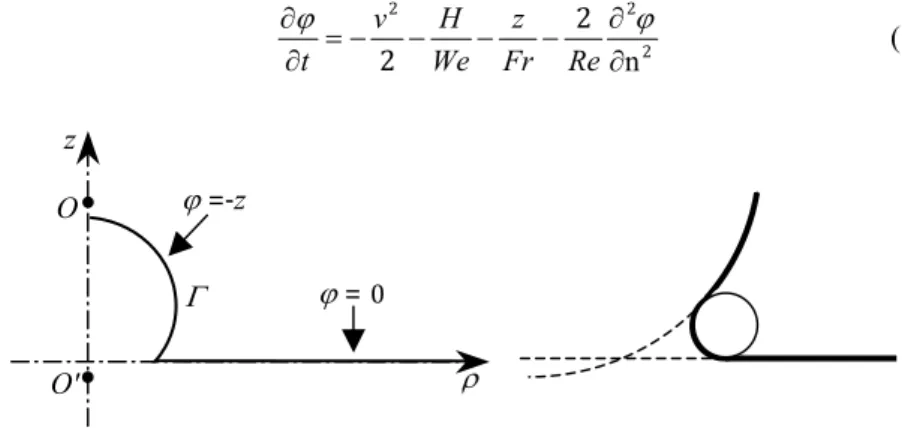
An axisymmetric liquid domain, bounded in the meridian plane (ρ,z) by the liquid-gas interface Γ is considered (Figure 2). Due to the impulsive nature of the

(8)

drop impact, an irrotational flow model is appropriate. A harmonic velocity potential subject to Dirichlet boundary conditions, can thus be defined. The local time derivative of the velocity potential is calculated by combining the normal momentum balance with the Laplace pressure jump to obtain the Bernoulli's equation. A dimensionless formulation is used:

2 2 2 ₂ 2 ∂n ∂ − − − − = ∂ ∂ϕ ϕ Re Fr z We H v t (19)

Figure 2: Initial geometry and potential. The neck region is smoothed. In this equation v is the dimensionless velocity, H is the total curvature and

Re, Fr and We are respectively the Reynolds, Froude and Weber numbers. The

drop radius R is adopted as length scale and σ Rρ_L as velocity scale, where σ

and ρL are the surface tension and the liquid density. The ratio between the

length and velocity scale gives the time scale. Viscous effects are partially taken into account as the normal viscous stress appears in eqn (19). The complete description of this model can be found in Georgescu et al. [2].

In order to avoid topological change, the falling spherical drop is initially placed in contact with the liquid surface. A negligibly small volume of the sphere is cut-out and, to avoid a singularity of the capillary pressure, the intersection of the sphere with the initially flat liquid surface is smoothed in the meridian plane by a circular element (Figure 2). The drop initially falls with a constant velocity onto an initially still liquid surface. The discontinuity of the velocity potential in the neck region is eliminated by means of the quadratic smoothing procedure described by Weiss and Yarin [10].

4.2 Solution procedure

The application represents a transient free-boundary problem that repeatedly involves two types of calculations: (a) solution of Laplace equation for normal components of the velocity, (b) updating of the potential at the forthcoming time step by using time marching scheme of Runge-Kutta and displacement of the interface.

Within the first type of calculation, the Laplace equation is solved by the Boundary Element Method using gradient formulation. First order elements are

(9)

used to approximate the unknowns. The vortex strength is calculated by interpolating the given velocity potential over the interface by the cubic splines. The solution is obtained by grouping source/vortex rings using multipole techniques discussed in previous section coupled with the GMRES iterative solver without preconditioning. In order to maximize the number of multipole calculations the multipole coefficients are calculated at two different expansion centres. Two expansion centres are used and their positions are evaluated at each time step, following the deformation of the interface. The normal velocity obtained at previous time step is used as an initial guess for the iterative solver for the subsequent time step.

Within the second type of calculation, the Bernoulli’s equation is solved by 4th_{order explicit Runge-Kutta scheme for the local time derivative of the}

velocity potential. The time steps are chosen according to the stability criterion described by Georgescu et al. [2]. The interface position is then updated according to the normal velocity component.

5 Results

The presented MM-BEM has been implemented for the axisymmetric static potential problems. With 18 terms in the expansion, this method provides accurate results when compared to analytical solution of Dirichlet or Neumann problems. The computational time is almost reduced by half when compared to the conventional BEM [7].

Figure 3: Comparison of numerical and experimental profiles (Fr=90, We=43) obtained by MM-BEM and Liow [11]. Bottom image reproduced with permission from Cambridge University Press.

(10)

The method is adapted for free surface flows and specifically to the chosen application of a drop impinging on a liquid surface. The number of nodes on the interface varies from 20 to 150 and the multipole series expansion is truncated after 21 terms. The comparison of the free surface profiles obtained by simulation through MM-BEM and experiments [11] at different instants are shown in Figure 3 (Fr=90, We=43). The qualitative agreement is correct.

Furthermore, a 10% of total CPU time saving is obtained when using MM-BEM instead of the conventional MM-BEM. Simulated profiles are identical in both methods.

6 Conclusion

A multipole based BEM has been implemented in an axisymmetric environment for the simulation of moving boundary problem of drop impact onto a liquid surface. By multipole techniques the interaction between individual nodes and ring sources in far field has been replaced by the interaction between node and group of ring sources. It has been shown that results obtained through MM-BEM matches well with available experimental data.

Although the time reduction is not significant yet, there is a wide scope of improvement in MM-BEM. The tuning of the parameters, for example, the number of terms in multipole series expansion, efficient choice of multipole centre in order to increase the validity of the far field and optimizing the admissibility criterion can further lead to more CPU time saving. To the best of our knowledge, this is the first attempt to accelerate the axisymmetric moving boundary value problem using a multipole expansion based technique.

References

[1] Oguz, H.N. & Prosperetti, A., Bubble entrainment by the impact of drops on liquid surfaces. Journal of Fluid Mechanics, 219, pp. 143–179, 1990. [2] Georgescu, S.C., Achard J.-L. & Canot, E., Jet drops ejection in bursting

gas bubble processes. European Journal of Mechanics B-Fluids, 21(2), pp. 265–280, 2002.

[3] Pozrikidis, C., Three-dimensional oscillations of inviscid drop induced by surface tension. Computer and Fluids, 30, pp. 417–444, 2001.

[4] Brebbia, C.A., Telles, J.C.F. & Wrobel, L.C., Boundary Element

Techniques, Springer-Verlag: Berlin and New York, 1984.

[5] Brockett, T.E., Kim, M-H. & Park, J-H., Limiting forms for surface singularity distributions when the field point is on the surface. Journal of

Engineering Mathematics, 23, pp. 201–31, 1989.

[6] Morse, P.M. & Feshbach, H., Methods of theoretical physics, McGraw-Hill: New York, 1953.

[7] J. Singh, A. Glière & J.-L. Achard, Multipole accelerated BEM for axisymmetric potential problem. (in preparation).

(11)

[8] Morton, D., Rudman, M. & Liow, J. L., An investigation of the flow regimes resulting from splashing drops. Physics of Fluids, 12(4), pp. 747– 763, 2000.

[9] Watanabe, Y., Saruwatari, A., & Ingram, D.M., Free-surface flows under impacting droplets. Journal of Computational Physics, 227(4), pp. 2344– 2365, 2008.

[10] Weiss, D.A. & Yarin A.L., Single drop impact onto liquid films: neck distortion, jetting, tiny bubble entrainment, and crown formation. Journal

of Fluid Mechanics, 385, pp. 229–254, 1999.

[11] Liow, J.L., Splash formation by spherical drops. Journal of Fluid