HAL Id: hal-01831318
https://hal.archives-ouvertes.fr/hal-01831318
Submitted on 20 Aug 2018
HAL is a multi-disciplinary open access
archive for the deposit and dissemination of
sci-entific research documents, whether they are
pub-lished or not. The documents may come from
teaching and research institutions in France or
abroad, or from public or private research centers.
L’archive ouverte pluridisciplinaire HAL, est
destinée au dépôt et à la diffusion de documents
scientifiques de niveau recherche, publiés ou non,
émanant des établissements d’enseignement et de
recherche français ou étrangers, des laboratoires
publics ou privés.
relation to visual sensory attributes: a new approach on
the rose bush for objective evaluation of the visual
quality
Morgan Garbez, R. Symoneaux, Etienne Belin, Y. Caraglio, Yann Chéné, N.
Dones, Jean-Baptiste Durand, G. Hunault, D. Relion, M. Sigogne, et al.
To cite this version:
Morgan Garbez, R. Symoneaux, Etienne Belin, Y. Caraglio, Yann Chéné, et al.. Ornamental plants
architectural characteristics in relation to visual sensory attributes: a new approach on the rose bush
for objective evaluation of the visual quality. European Journal of Horticultural Science, Ulmer, 2018,
83 (3), pp.187-201. �10.17660/eJHS.2018/83.3.8�. �hal-01831318�
V o l u m e 8 3 | I s s u e 3 | J u n e 2 0 1 8 187
Ornamental plants architectural characteristics in relation to
visual sensory attributes: a new approach on the rose bush for
objective evaluation of the visual quality
M. Garbez
1,2, R. Symoneaux
3, É. Belin
4, Y. Caraglio
5, Y. Chéné
4, N. Donès
6, J.-B. Durand
7,8, G. Hunault
9,
D. Relion
1, M. Sigogne
1, D. Rousseau
10and G. Galopin
11 IRHS, INRA, Agrocampus Ouest, Université d’Angers, Beaucouzé, France 2 Pépinières Desmartis, Bergerac, France
3 Unité de Recherche GRAPPE, Université Bretagne Loire, Ecole Supérieure d’Agricultures (ESA), INRA, Angers, France 4 Université d’Angers, Laboratoire Angevin de Recherche en Ingénierie des Systèmes (LARIS), Angers, France
5 AMAP, CIRAD, CNRS, INRA, IRD, UM, Montpellier, France 6 PIAF, INRA, UCA, Clermont-Ferrand, France
7 Virtual Plants, Montpellier, France
8 Laboratoire Jean Kuntzmann, MISTIS, INRIA Grenoble – Rhône-Alpes, Saint Ismier, France
9 Université d’Angers, Laboratoire Hémodynamique, Interaction, Fibrose, et Invasivité Tumorale Hépatique (HIFIH), Angers,
France
10 Université de Lyon, Centre de Recherche en Acquisition et Traitement de l’Image pour la Santé (CREATIS), Villeurbanne,
France
Original article – Thematic Issue
Summary
Within ornamental horticulture context, visual quality of plants is a critical criterion for consumers looking for immediate decorative effect products. Studying links between architecture and its pheno-typic plasticity in response to growing conditions and the resulting plant visual appearance represents an interesting lever to propose a new approach for man-aging product quality from specialized crops. Objec-tives of the present study were to determine whether architectural components may be identified across different growing conditions (1) to study the archi-tectural development of a shrub over time; and (2) to predict sensory attributes data characterizing multi-ple visual traits of the plants. The approach addressed in this study stands on the sensory profile method using a recurrent blooming modern rose bush (Rosa
hybrida ‘Radrazz’) presented in rotation using video
stimuli. Plants were cultivated under a shading gra-dient in three distinct environments (natural condi-tions, under 55 and 75% shading net). Architecture and video of the plants were recorded during three stages, from 5 to 15 months after plant multiplication. Except for visual traits at the scale of the organs, pan-el performance was highly satisfying for most of the sensory attributes listed. Strong correlations (Spear-man’s coefficient ranging from 0.72 to 0.98) were found between them and architectural variables ex-tracted from phytomer to plant scale data. Acceptable to very satisfying models were obtained (Q2 ranged
from 0.49 to 0.95, normalized RMSEP <17.3%) with simple ordinary least squares regression and vari-able transformation to encompass non-linear rela-tionships. The proposed approach presents therefore a powerful way to gain a better insight into the ar-chitecture of shrub plants together with their visual
Significance of this study
What is already known on this subject?• Visual quality of ornamental plants is a key parameter playing a major role in the purchase triggering for consumers. Nonetheless, it is a complex notion based on the individual and subjective appreciation. What are the new findings?
• A new method to studying and modeling the relationships between ornamental plant architecture and main visual components. The obtained models enabled to identify architectural variables with good predictive ability and especially relevant for explaining the visual appearance of the architecture of rose bush. What is the expected impact on horticulture?
• Within ornamental horticulture context, visual quality of plants is an important criterion for consumers looking for immediate decorative effects products. This work will make it possible to objectify the relation between the architecture of the plant and the visual perception by the consumer. It’s a future tool to help innovation in ornamental horticulture.
German Society for Horticultural Science
appearance to target processes of interest in order to optimize growing conditions or select the most fitting genotypes across breeding programs, with respect to contrasted consumer preferences.
Keywords
architectural analysis, linear regression, Rosa hybrida, sensory profile, visual appearance, woody ornamental plant
188 E u r o p e a n J o u r n a l o f H o r t i c u l t u r a l S c i e n c e
Introduction
Visual quality of ornamental plants is a key parameter playing a major role in the purchase triggering for consum-ers (Townsley-Brascamp and Marr, 1994; Schreiner et al., 2013; Ferrante et al., 2015). Nonetheless, it is a complex notion based on the individual and subjective appreciation of the product design or appearance by a given individual. Thus, preferences are mainly related to aesthetical judg-ments, although, for objective or subjective reasons, there may be differences or conflicts of judgment between people (Higginbotham, 1987; Creusen and Schoormans, 2005; Bou-maza et al., 2010).
Effects of growing practices evaluated on various plant parameters measured with destructive or contactless meth-ods are rather well-documented (Ferrante et al., 2015). None-theless, in such studies, a plant with pleasant visual appear-ance is too often seen as univocal and consumer preferences as homogeneous. Therefore even if manual or automatized grading occurs, actually the likeliness to observe a simple re-lation and good concordance between visual quality grades with specific preferences and expectations of the consumers, is small (Kohsel and Bennedsen, 2001; Garbez et al., 2016). From past decades, quality management of fresh horticultur-al products, especihorticultur-ally fruits and vegetables, strongly bene-fited from the sensory evaluation science (Meilgaard et al., 2006). Its recent application on the rose bush showed also the strong relevance for providing a common background for objectifying and harmonizing visual quality studies on orna-mental plants using real plants (Boumaza et al., 2009), single plant facet pictures (Boumaza et al., 2010; Huché-Thélier et al., 2011; Santagostini et al., 2014), and virtual plants pre-sented in rotation on video (Garbez et al., 2015, 2016).
However, nowadays ornamental woody plants are still very often subjected to pruning or growth regulator appli-cations to modulate plant growth for an empirical control of their quality. Knowledge about the variability of the archi-tectural responses against environmental factors represents a valuable way to better control plant visual appearance with more reasoned, cheaper, and greener growing practices (Galopin et al., 2010; Huché-Thélier et al., 2011; Morel et al., 2012; Demotes-Mainard et al., 2013b; Crespel et al., 2014; Li-Marchetti et al., 2015). Understanding and controlling ar-chitecture is therefore an interesting lever to address orna-mental plant design management, and more specifically to better fulfill expectations of the consumers thanks to knowl-edge about their requirements. Detecting links between ar-chitectural parameters and hedonic-free assessments of
vi-sual traits is thus needed to investigate if putative underlying key biological processes could be targeted. This approach, necessary to address visual quality of ornamental plants, cannot remain empirical. Thus, identification of visual at-tributes is necessary on the one hand to analyze their rela-tions with the architectural components, the subject of this publication, and on the other hand to further understand the preferences of the consumers. However, literature about re-lations between perception of plant visual appearance traits and such architectural parameters for explaining consumer preferences is still poorly documented (Scuderi et al., 2012). First studies on rose bushes demonstrated the high poten-tial of this approach through correlative studies either using young plants, or addressing for specific aims a limited num-ber of visual descriptors selected from a sensory method or picked out from UPOV guideline for Rosa L. (Huché-Thélier et al., 2011; Crespel et al., 2013; Santagostini et al., 2014).
The main research objectives addressed in the present study concern (1) the architectural characterization over time of the rose bush without any pruning so that all the po-tential basal sprouts can be taken into account, and (2) if ar-chitectural components can be identified in relation to some visual traits and used for predicting them independently of plant age and growing conditions. The same rose bush cul-tivar was grown under three contrasted shading conditions to induce phenotypic variability. The architecture of the plants was recorded three times over 15 months of cultiva-tion. In parallel, visual traits of the plants were characterized through a sensory profile trial using videos presenting them in rotation as stimuli. The paper presents: (1) the sensory profile of the plants on videos using multiple sensory attri-butes describing general aspects of the plants and their or-gans; (2) the architectural monitoring over the three acqui-sition stages, and the generation of plant-scale architectural variables; for (3) a correlation and ordinary least square regression study with the aim to predict the relevant and consensual sensory attributes using architectural variables as predictors.
Materials and methods
Plant material
The experiment used recurrent-flowering rose bushes from the Radrazz cultivar (Rosa hybrida L. ‘Radrazz’, mar-keted under Knock Out®) and light intensity as a means of
inducing consequent phenotypic differences between plants. ‘Radrazz’ is a modern shrub cultivar. The flower is terminal,
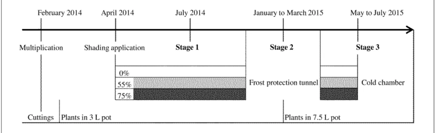
Figure 1. Schematic presentation of the container cultivation cultural conditions of ‘Radrazz’ rose bushes and stages of data
acquisition periods.
FIGURE 1. Schematic presentation of the container cultivation cultural conditions of ‘Radrazz’ rose bushes and stages of
V o l u m e 8 3 | I s s u e 3 | J u n e 2 0 1 8 189 solitary and simple, red to pink Bengali flowers – red45A,
with determinate growth (Morel et al., 2009). Plants were obtained from single node cuttings harvested on the 4th
February 2014 and individually placed in plugs for rooting as described in teammate protocols (Morel et al., 2012; De-motes-Mainard et al., 2013b).
Growth conditions
Plants were cultivated outdoors in pots under three shading levels in the experimental facilities of the IRHS (French Research Institute on Horticulture and Seeds, An-gers, France; 47°28’45.8”N, 0°36’32.3”W, altitude 48 m).
As represented in Figure 1, experimental conditions started on the 25th April 2014, with young plants in 3-L pot,
aged 81 days since cutting. Harvest was chosen as time refer-ence for dating plant age. Sixty flowering and homogeneous plants intended to be characterized were randomly and evenly assigned in three environments on a soilless culture ground: (1) without shading screen (denoted 0%); (2) under
a tunnel covered with a 55%; or (3) 75% shading screen. The first year the plants were placed at a density of 1.1 plant m-².
Then at mid-December 2014, plants were moved to an un-heated polyethylene tunnel to prevent any frost damages on roots and future young shoots. Plants were then repotted in 7.5-L pot. Finally, plants were replaced on the 25th
Febru-ary 2015 to their respective environment at a lower density (0.8 plant m-²).
Plants were potted in a well-draining substrate (custom mix made by Faliénor; Vivy, France) composed of Irish peat, perlite, coir (50:40:10 in volume ratio), and fertilized with 1 kg m-3 of PG-Mix™ 14-16-18. Watering schedules of the three
environments were individually adjusted according to rain, microclimatic conditions and substrate moisture status of the plants to guarantee no water limitation. Water was com-pleted for fertigation with liquid 3:2:6 N-P2O5-K2O ratio
solu-tion (Plant-Prod® 15-10-30; Plant Products, Leamington, ON,
USA) with adjusted pH at 6.5 and EC at 1.2 mS cm-1.
16
FIGURE 2. Panel of cropped and reduced size images of three rose bushes from the different shading environments (from left to right: 0, 55, and 75% of shading) over the three acquisition stages (from top to bottom: S1, S2, S3), then manually defoliated at the third stage (S3D).Figure 2. Panel of cropped and reduced size images of three rose bushes from the different shading environments (from left
to right: 0, 55, and 75% of shading) over the three acquisition stages (from top to bottom: S1, S2, S3), then manually defoliated at the third stage (S3D).
190 E u r o p e a n J o u r n a l o f H o r t i c u l t u r a l S c i e n c e
Table 1. Number of samples for architectural recording, image capture and video editing for each shading environment and
for the three stages. Stages
Shading levels Plant age Video Sensory Architecture Relation1
Stage 1 5 months 59 57 53 52: 36/16 0% 19 19 18 17: 12/5 55% 20 19 17 17: 12/5 75% 20 19 18 18: 12/6 Stage 2 12 months 60 57 46 45: 30/15 0% 20 19 16 15: 10/5 55% 20 19 15 15: 10/5 75% 20 19 15 15: 10/5 Stage 3 15 months 60 57 33 33: 24/9 0% 20 19 11 11: 8/3 55% 20 19 11 11: 8/3 75% 20 19 11 11: 8/3 Total 179 171 132 130: 90/40
1 First number indicates the number of plants characterized at both sensory and architectural levels; the second and third numbers separated by a
slash detail respectively the number of observations used for calibration and for validation of the predictive models.
Plant acquisitions
Tree times, a double characterization was realized during the 15 months: visual appearance, through a sensory profile using as stimuli rotating plant video edited from image se-quences; and architecture, using a 3D magnetic digitizing contact method (Figure 1). For the three stages of develop-ment and the three shading environdevelop-ments, 179 rotating plant video and 132 plant architecture records were obtained for subsequent characterizations.
1. Image capture and editing of rotating plant videos.
A specific enclosure was set for capturing images sequences of potted plants in rotation. It was composed of a metallic structure (2.25 m height × 3 m width × 6 m length) covered with an occulting black fabric to avoid uncontrolled light variations, a blue photographic cloth (DynaSun, W003; Con-fidence Europe GmbH, Essen, Germany) for background, and a carpet of similar colour on the floor. Plant rotation and im-age capture were computationally controlled through a us-er-interfaced turntable (custom built device; Forumgraphic SA, Cassis, France). In order to obtain comparable images across data collection, system parameters were chosen and fixed for all the experiment duration testing the image cap-ture on potted rose bushes of different ages from other ex-periments.
Center of the turntable (height of 30 cm) was placed at 1.4 m from the background, and 4.5 m from a front 12 bits 10Mpx CMOS colour camera (GigE UI-5490SE; IDS Imaging Development Systems GmbH, Obersulm, Germany) placed at 70 cm height from the floor. Focus was achieved with a stan-dard zoom lens (Tevidon® 2/10; Docter Optics Components
GmbH, Neustadt an der Orla, Germany). Scene illumination was controlled with daylight lamps (temperature colour ranging from 5500 to 6500 °K): four linear LED lamp lines in lateral position surrounding the turntable, two superior fluorescent tubes, and an annular LED lamp around the cam-era to enhance front lighting. Light variations in the scene were assessed and reduced using two-dimensional graphs of pixel intensities from the ‘plot profile’ function of ImageJ (Abràmoff et al., 2004) on greyscale images of the plant-less scene. Parameters for plant image sequence capture were set to: 360 images (resolution of 3840×2748) obtained along rotation intervals of one degree with break of seven seconds
for plant stabilization before image capturing. The time to capture a complete plant image sequence was thus fixed to 42 minutes. Before each sequence acquisition, the image of the blue background with the turntable and a plant-less pot filled with substrate was recorded for image analysis purpos-es.
Once the image sequences for the last stage (S3) were obtained (Figure 2), all the sequences were converted in AVI videos using ImageJ (Appendix A). Video parameters chosen were 3° between consecutive frames, thus 120 images per plant, with a frame rate of 10 frames s-1 and JPEG
compres-sion.
2. Plant architecture recording. Rosa plants present stems
with defined growth by terminal flowering (or abortion), and subsequent sympodial branching in all axes. For recurrent flowering varieties as ‘Radrazz’, axes are modules with con-tinuous growth composed of phytomers edified by a single terminal meristem in which organogenesis ceases with au-tonomous floral induction (Zieslin and Mor, 1990; Le Bris et al., 1998; Morel et al., 2009; Costes et al., 2014). The phy-tomer is the basic structural and functional unit of vascular plant body. Generated by apical meristem of the shoots, the phytomers form the leafy axes by superposition, and higher order axes through branching resulting mostly from the out-growth on node region of lateral bud(s) inserted at the leaf axil(s) (Barthélémy and Caraglio, 2007).
Plant architecture recording was done using the PiafDigit software (Donès et al., 2006). It consisted of encoding with a Fastrack® 3D digitizer (Polhemus, Colchester, VT, USA) the
3D coordinates of the phytomers constituting all apparent plant axes together with their topological relation (succes-sion or branching) and some morphological features (Cre-spel et al., 2013; Morel et al., 2009, 2012; Li-Marchetti et al., 2015). Branching order notation followed the ‘birth’ organi-zation of the axes, i.e., the first axis sprouting from the cut-ting was denoted as the 1st branching order, its lateral buds
growth leading to second branching order axes and so on. This primary structure was labeled in this study as the ‘ele-mentary architectural system’. Proximal axes sprouting at or under the substrate level, sometimes called ‘renewal canes’ (Zieslin and Mor, 1981) and empirically seen as total reiter-ated complexes (Costes et al., 2014; Kawamura et al., 2015)
V o l u m e 8 3 | I s s u e 3 | J u n e 2 0 1 8 191 of an ‘elementary architectural structure stage’ (Crespel et
al., 2013; Li-Marchetti et al., 2015), were denoted also as first branching order axes. These axes and all their descendants were further labeled as forming the ‘delayed architectur-al systems’. Morphologicarchitectur-al features consistently recorded throughout the experiment consisted of reporting the apex state of the axes, and measuring with a digital caliper the basal diameter of each first branching order and the mid-length diameter for all the axes.
Plant characterizations
1. Visual characterization. Following an adaptation
of Garbez et al. (2016) and Huché-Thélier et al. (2011), 171 different videos for the same 19 plants by shading
environ-ments, at the three acquisition dates (Table 1), were select-ed as the products to be visually characterizselect-ed by a trainselect-ed panel of 20 subjects according to a sensory profile approach derived from the quantitative descriptive analysis (QDA®)
method (Stone et al., 1974). During the panel formation (10 hours divided into five sessions), 17 sensory attributes were elicited for describing the plants (Table 2): 12 were re-lated to plant general aspect traits: the volume, the height, the width of the plant; the quantities of branching, quantity of leaves, flowers, fruits, and carrier axes; the growth habit, the shape uniformity, the shape balance, and lastly the plant density. Five other attributes described organ properties within the plant: the size and the colour of the leaves, the height of the flowers within the plant, the height of the
veg-Table 2. Sensory attribute definitions and panel performance indices. The first block of rows reports the consensual attributes
with the best panel performance; the second reports those with unsatisfying performance indices highlighted in italic characters.
Sensory
attribute Definition Repeatability1 Reproducibility2 Consonance (%)
Discriminating power (F-ratio) Flowers3 Quantity of flowers: (0) no flower to (10) very high amount of
flowers 0.54 ± 0.07 0.52 ± 0.46 93.2 15.5
***
Height Plant height from collar: (1) very small to (10) very tall 0.60 ± 0.02 0.84 ± 0.15 88.4 55.5***
Width Plant width along rotation: (1) very thin to (10) very wide 0.71 ± 0.04 1.00 ± 0.18 76.9 8.1***
Density Plant density: (1) very loose, large and numerous holes within the plant silhouette to (10) very dense, any holes within the plant silhouette
0.71 ± 0.05 1.45 ± 0.32 69.6 7.5***
Leaves3 Quantity of leaves: (0) no leaf to (10) very high amount of
leaves 0.76 ± 0.05 0.89 ± 0.49 79.4 8.1
***
Volume Volume of the shape delimited by the plant contour: (1) very
small to (10) very large volume 0.77 ± 0.04 1.03 ± 0.21 84.4 10.6
***
Carriers Quantity of strong carriers axes: (0) no carrier axis to (10) very
numerous carrier axes 0.79 ± 0.07 1.21 ± 0.23 72.3 8.1
***
Fruits Quantity of fruits: (0) no fruit to (10) very high amount of fruits 0.80 ± 0.10 1.09 ± 0.35 83.4 12.8***
Branching Quantity of branches: (0) no branch to (10) very high amount of
branches 0.82 ± 0.09 1.14 ± 0.25 78.4 4.0
***
Balance Balance of the plant silhouette shape: (1) very unbalanced and dissymmetric to (10) very balanced plant evenly developed with constant shape along the rotation
0.93 ± 0.13 1.49 ± 0.29 65.2 10.6***
Habit Growth habit, shape elongation of the plant: (1) very spreading
habit to (10) very upright habit 0.98 ± 0.07 1.09 ± 0.21 64.1 26.0
***
Flower
height3 Height of the flowers in the plant: (1) very down to (10) very high in the plant 0.77 ± 0.07 0.68 ± 0.66 77.9 43.6 ***
Growth
height Height of the growth organs (axes or both axes and leaves if present) in the plant: (1) very down in the plant to (10) very high in the plant
0.83 ± 0.10 0.88 ± 0.35 42.5 6.3***
Leaf size3 Average size of the leaves: (1) very small to (10) very large
leaves 0.88 ± 0.10 1.02 ± 0.52 36.3 6.9
***
Leaf colour3 Green darkness of mature leaves: (1) very clear to (10) very
dark leaves 0.93 ± 0.08 1.32 ± 0.54 53.3 3.2
***
Flower
clustering3 Proximity of the flowers: (1) not particularly grouped, very homogeneously distributed in the plant to (10) flowers forming
only one distinct cluster
1.12 ± 0.13 0.89 ± 0.90 82.4 39.7***
Uniformity Complexity of the plant shape formed by the growth organs: (1) very irregular with several distinct blocks to (10) very regular forming an indivisible shape
1.17 ± 0.12 1.66 ± 0.37 60.8 9.0***
1 Values are means ± standard errors over the 8 duplicated videos of the pooled standard deviations of the subject scores between replications. 2 Values are means ± standard errors over the 171 different videos of the standard deviations of the subject scores.
3 Attributes for which the score 0 means no corresponding organ in the plant, and thus for which videos of the plants during winter rest (Stage 2)
192 E u r o p e a n J o u r n a l o f H o r t i c u l t u r a l S c i e n c e etative organs (leaf and axes, or axes only) within the plant,
and the clustering of the flowers. All the 171 products and four duplicates for repeatability controls, next to 31 other plant videos used for another purpose not dealt with here, were scored upon the 17 attributes on paper sheets by the 20 subjects in 8 scoring sessions of an hour in average (25 to 27 videos to score per subject and session). Formation and scoring sessions took place in a computer lab with identical LCD monitors in standard mode configuration with optimal preset 1920×1080 resolution, and situated to avoid commu-nication between subjects. Subjects were not informed about cultural conditions and ages of the plants. All the videos and their duplicates were anonymized with three-digit number codes. Thus for each plant, the videos presenting respective-ly its three acquisition stages can also be considered as three different plants.
To limit the task difficulty for the panelists, scoring ses-sions consisted in the characterization of two out of three consecutive batches of videos: a first batch formed with
plants presenting leaves and flowers (S1 and S3 pooled), and a second formed either with videos of plants during rest phase (S2) or with flowering plants before manual defolia-tion after the image acquisidefolia-tion for S3 and not dealt with here (Figure 2). Videos were presented using VLC media player (VideoLAN project, France) and individual playlist scripts according to an optimal design based on a William’s Latin square adaptation and randomization to prevent any order effect.
Performance of the panel for each sensory attribute was assessed with common approaches presented in pre-vious studies using rose bushes (Boumaza et al., 2010; Huché-Thélier et al., 2011; Santagostini et al., 2014; Garbez et al., 2015). Repeatability and reproducibility (Rossi, 2001) of average measurements over products were used respec-tively to assess the ability of the subjects to score consis-tently for the duplicated videos, and to score the products as the other panel subjects. The agreement between subjects was analyzed through principal component analysis (PCA),
Table 3. Standardized principal component analysis of weighted determined axis pooled observations (n=33,690) with
axis-scale data extracted from plant architectures recorded during all the experiment. The first block of rows reports quantitative variables and Pearson correlations with principal components (PC) if not negligible (N if rP<0.3 in absolute value). The second
block reports variables characterizing the axes and conditions treated as supplementary qualitative data with eta-squared indices measuring the proportion of variance explained on PC.
Data type – Variable Category PC1 PC fulfilling Kaiser criterion and variance explained (%)
(37.6%) (23.3%)PC2 (12.8%)PC3
Quantitative data
Length Morphology 0.92 N N
Number of phytomers Morphology 0.88 N N
Median diameter Morphology 0.78 N N
Number of branched nodes Morphology 0.74 N N
Relative location of branching insertion1 Geometry -0.69 N N
Curvature2 Geometry -0.65 N N
Cord2 angle with the vertical Geometry N 0.62 N
Lateral distance of the insertion3 Geometry -0.60 0.46 0.64
Lateral distance of the extremity3 Geometry N 0.60 0.74
Vertical distance of the insertion3 Geometry N -0.89 0.38
Vertical distance of the extremity3 Geometry N -0.86 0.34
Azimuth4 Geometry - -
-Basal diameter5 Morphology - -
-Qualitative data
Elementary versus delayed systems Topology 0.01 0 0.15
Branching order Topology 0.33 0.02 0.12
Apex state Morphology 0.05 0.04 0.05
Stage Condition 0.01 0.01 0.08
Shading Condition 0 0.02 0.03
Stage: Shading Condition 0.01 0.04 0.12
Stage: Plant Condition 0.02 0.1 0.17
Plant Condition 0.01 0.05 0.09
1 Computed as the ratio between length of the portion from the base of the bearing axis to the insertion point of the axis in question and the total
length of the bearer. It thus tends to 0 if the axis is a basal branching and to 1 if it is apical one. The ratio was set to 0 for all the branching order 1 axes.
2 Computed as 1 minus the ratio between axis cord length: the axis cord is the straight line from the base to the extremity of the axis; and the axis
length. It thus equal to 1 for axes completely recurved, and tends to 0 for straight axes.
3 Distances are computed from the plant collar to the point mentioned in the variable name.
4 Not considered in the multivariate analysis since azimuth of the axes cannot be individually compared between plants, but only extracted for
plant-scale variables.
V o l u m e 8 3 | I s s u e 3 | J u n e 2 0 1 8 193 with subjects as columns and products as rows, to
high-light outlying subjects and compute a consonance measure-ment of the scores as the variance accounted for the first PC (Dijksterhuis, 1995). Finally, score differences between prod-ucts were assessed by four-way mixed analysis of variance (ANOVA) modeling (Kuznetsova et al., 2015). The analysis model included the subjects as a random factor with stages and shading environments as fixed factors, plants as a nest-ed and fixnest-ed factor within shading environments, and their interactions. Significance of the score differences between products was used to evaluate the discriminating power of the attributes and the global panel performance. This was tested through the effect on scores of the three-way interac-tion between plants in shading levels and stages. Discussions were undertaken for discarding attributes for which the pan-el performance components were eventually judged as not sufficient. Then, PCA of the ‘products × attributes’ matrix of average scores was carried out to achieve a synthetic de-scription of the relationships between the attributes, and of the visual characteristics of the plants presented on videos.
2. Architectural characterization for generating plant architectural descriptors. Architectural records were
converted into MTG files (Multi-scale Tree Graph; Godin and Caraglio, 1998) through PiafDigit for extracting axis-scale variables using the amlPy interface module under the OpenAlea platform (Bonnard and Pradal, 2008; Pradal et al., 2008; Morel et al., 2009; Crespel et al., 2013). Variables extracted concerned the morphology, the topology and the geometry of the axes complemented with experimental information (plant index, shading level and stage of acquisition; Table 3).
Effectiveness of the architectural differences between the shading treatments over stages was assessed considering the determined axis observations, i.e., the axes which organo- genesis has been stopped by floral transformation of their apex. Blind shoots were considered as determined axes too since apical meristem abortion also implies the arrest of the axis organogenesis. Branching (number of axes) and organo-genesis (number of phytomers) were analyzed separately by mixed ANOVA modeling and Bonferroni’s correction method for post hoc tests with error level α=0.05. Models included stages and shading environments as fixed factors, plants as a nested random factor within the shading environments, and their interactions.
Extracted axis-scale variables were then subjected to PCA to analyze major variation sources between determined axis observations (Morel et al., 2009), and further used to generate a database of plant-scale variables that can be po-tentially related to the studied visual traits. Plant-scale vari-ables selected by Crespel et al. (2013) and used in Li-Mar-chetti et al. (2015) were straightforwardly extracted for comparison purposes. Other variables integrating axis-scale variables at the plant level were defined with descriptive statistics such as sum, mean, median, quantiles, ranges, em-pirical standard deviation, minimum, maximum and coeffi-cient of variation, according to the relevance of their use. The most important quantitative axis-scale variable highlighted by PCA was used to generate a supplementary qualitative variable determined from comparative analysis of different clustering and validation approaches. This qualitative vari-able was used like the branching order and the apex state to generate other more detailed variables. In parallel, the 3D coordinates of phytomers were extracted from the MTG files to be analyzed individually as 3D point clouds under the R environment (R Development Core Team, 2015).
Ba-sic functions as for integration of the axis-scale variables en-abled the computation of other features at whole-plant scale, such as landmark coordinates, metric distances, and spatial variances characterizing the phytomer cloud of the plants. In addition, volumetric estimation of the plants was obtained though computing the 3D convex hull volume enclosing the phytomers using the alphahull R package (Pateiro-López and Rodrıguez-Casal, 2010). Finally, the database integrated also some complementary variables built on previous ones. Thus, more than a thousand plant-scale architecture-based vari-ables (p=1,209) were collected and available as potential predictors for relationship study with the sensory attributes (categorization of the variables and examples in Table 4).
3. Relating visual and architectural characterizations.
Out of the 171 products characterized by sensory profile, 130 corresponding plant architecture recordings were avail-able (Tavail-able 1). Sensory attribute variavail-ables were defined as the average scores of the subjects by product and analyzed conjointly with plant-scale architectural descriptors. Links between pairs of sensory attribute variables and plant archi-tectural descriptors were first evaluated with Spearman’s correlation coefficient (rS) to detect eventual monotonic
rela-tionships (Huché-Thélier et al., 2011; Santagostini et al., 2014). Then, prediction of the sensory attributes variables was tested with simple linear regression through ordinary least squares (OLS), the most common and simple regression method (Næs et al., 2011; Kuhn and Johnson, 2013), using the plant architectural descriptors as potential predictors one by one without any stage- or shading-based parameters.
In order to assess their relevance and genericity, the models were first calibrated through 10 repeats of 10-folds cross-validation on two-thirds of the data (n=90 plants ob-servations over stages and shading environments), and then validated on the remaining third (Borra and Di Ciaccio, 2010; Kuhn and Johnson, 2013). Data partitioning was the same for all the sensory attributes, i.e., with a balanced-based design according to stages and shading environments with a 2:1 ratio random sampling within all the 9 crossed conditions (Table 1). Goodness of fit was evaluated with the tradition-al coefficient of determination and lack of fit with the root mean square error for the entire calibration data (respective-ly R² and RMSE), and through 10-10 folds cross-validation (respectively R2
CV and RMSECV). Coefficients of determination
and root mean square error of prediction computed from the validation dataset (respectively Q2 and RMSEP) were
then used to assess the predictive ability of the models with unknown data. Common transformations (power, root, log, exponential and inverse) and normality supervised pow-er-transformations of Yeo-Johnson were applied to the pre-dictors (Yeo and Johnson, 2000) with the aim to better satisfy required linear modeling assumptions (Kuhn and Johnson, 2013) while exploiting more deeply the data still using a rel-atively simple modeling approach.
Statistical analyses
Statistical analyses were conducted under the R envi-ronment (R Development Core Team, 2015) with additional functions from the packages detailed thereafter. PCA were conducted with FactoMineR (Husson et al., 2016) using cen-tered and scaled data. Variable discretization was performed with classInt (Bivand et al., 2015), by increasing number of classes through k-means (Steinley, 2006) and Fisher-Jenks algorithms (Murray and Shyy, 2000; Anchang et al., 2016). Quality and stability of the solutions were assessed using elbow graphical method, clusterwise Jaccard similarity
sta-194 E u r o p e a n J o u r n a l o f H o r t i c u l t u r a l S c i e n c e tistics under bootstrap resampling with fpc (Hennig, 2008,
2015), and Davies-Bouldin cluster separation measure-ments (Davies and Bouldin, 1979) with clusterSim (Wale-siak and Dudek, 2015). Mixed models were designed using lme4 (Bates et al., 2016) and analyzed with ANOVA function of car (Fox et al., 2016) with type II sums of squares proce-dure (Langsrud, 2003). Subsequent multiple comparisons were done according to the Bonferroni’s adjustment method on least-squares means from lsmeans (Lenth, 2016). When required, Kenward-Roger’s degrees of freedom estimations were used for statistical inferences (Spilke et al., 2005; Kuznetsova et al., 2015). Data partitioning and modeling be-tween sensory and architectural data were done using caret (Kuhn, 2016).
Results
Visual characterization
All the attributes were significantly discriminant (the product effect, i.e. the interaction ‘plant : shading : stage’, was highly significant with p-value <0.001) indicating thus a relatively acceptable global panel performance (Table 2). Means and standard errors of repeatability measurements for all the attributes except ‘uniformity’ and ‘flower cluster-ing’ were relatively low and not so variable (maximum M = 1.17 and maximum SE = 0.13), indicating very little and sim-ilar differences of the subject scores over duplicated videos. Reproducibility measurements indicated that differences be-tween subject scores on same videos were also rather low
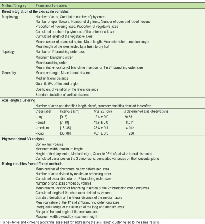
Table 4. Examples of architectural variables at plant-scale gathered according to methods used and description categories
proposed from the 1209 variables extracted. Method/Category Examples of variables
Direct integration of the axis-scale variables
Morphology Number of axes, Cumulated number of phytomers
Number of open flowers, Number of dry fruits, Number of open and faded flowers Proportion of flowering axes, Proportion of vegetative axes
Cumulated number of phytomers of the determined axes Cumulated length of the vegetative axes
Mean number of branched nodes, Mean length, Mean diameter at median length Mean length of the axes ended by a fresh to dry fruit
Topology Number of 1st branching order axes
Maximum branching order Mean branching order
Mean relative location of branching insertion for the 2nd branching order axes
Geometry Mean cord angle, Mean lateral distance Median lateral distance
Quantile 5% of the cord angle
Coefficient of variation of the lateral distance Standard deviation of vertical distance
Axis length clustering
Number of axes per identified length class1, summary statistics detailed thereafter
Class label Intervals (cm) M ± SE (cm) n determined axis observations
- tiny [0; 7] 2.4 ± 0.0 20.551
- small [7; 18] 11.9 ± 0.0 8.011
- medium [18; 35] 23.8 ± 0.1 4.202
- long [35; 88] 46.1 ± 0.3 926
Phytomer cloud 3D analysis
Convex hull volume
Maximum width, maximum height
Height of the barycenter, Median height, Quantile 95% of pairwise lateral distances Cumulated variances on the 3 dimensions, cumulated variances on the horizontal plane
Mixing variables from different methods
Mean number of phytomers on tiny determined axes Number of axes divided by maximum branching order Cumulated basal diameter of 1st branching order axes
Number of long axes divided by volume
Mean relative location of branching insertion of the 2nd branching order long axes
Cumulated length of the short axes divided by volume Standard deviation of the lateral distance of the medium axes Mean curvature of the 1st and 2nd branching order long axes
Interquartile range of the azimuth of the long and medium axes Range of the cord angle of the medium axes
Maximum width divided by maximum height
V o l u m e 8 3 | I s s u e 3 | J u n e 2 0 1 8 195 and stable except for ‘uniformity’, ‘flower clustering’, ‘flower
height’, ‘leaf colour’, and ‘leaf size’ (M over 1.50; SE over 0.50), indicating more relative differences between subject scores on same videos, eventually coupled with difference inconsis-tencies between the videos and the subjects. Finally, accept-able to very high consonance measurements confirmed with previous results the very good performance and consensual appropriation of the 11 other attributes out the 17 (Table 2).
Principal component analysis (PCA) of the average score matrix for the 171 products and the 11 selected sensory attributes allowed to identify some relations between visu-al characteristics, and to highlight how they structured the plants throughout shading environments and vegetation stages (Figure 3). Four principal components (PC) were con-sidered according to the Kaiser criterion, which explained 93.4% of the overall variance. However the first plan ac-counted for 70.9% and was sufficient to well discriminate main characteristics of the plants within stages and shading environments. Globally, PC1 and PC2 structured the plants according to V-shaped patterns separating the plants charac-teristics chronologically, and then with large to more subtle differences between shading levels. PC1 (45.8% of the vari-ance) synthesized plant dimensions, branching and shape equilibrium over stages, with the shading level diminution. Not surprisingly, it reflected very high to moderate correla-tions between ‘branching’ and ‘carriers’, ‘volume’, ‘width’, and ‘height’, and then ‘balance’. Highest Pearson correlations for ‘balance’ were with carriers (rP = 0.62) and branching (rP =
0.60) which presented the strongest association (rP = 0.92)
between all attributes pairs. Plant characteristics were es-sentially structured by age and sub-structured by shading level diminution. Interestingly, scores for plants grown under 75% of shade were systematically lower than those grown under 0 and 55% which were more similar. PC2 (25.1%) strongly reflected the expected very high correlation between ‘leaves’ and ‘flowers’, and their respective high and moderate correlation with plant density. PC2 opposed those attributes to ‘fruits’ and ‘habit’ presenting a negligible correlation (rP =
0.25), and ‘height’ also moderately reflected on PC2, with the
strongest correlation observed between ‘fruits’ and ‘leaves’ but with a low opposition link (rP = -0.42). It thus showed
a structuration of the products according to the presence or absence of leaves and flowers, separating, as expected, S1 and S3 far from S2 plant characteristics. Then, it showed also a sub-structuration within stage groups according to the quantity of leaves and flowers for S1 and S3; and according to density, habit, fruits and height for the three stages enabling
17
FIGURE 3. Biplot of the standardized principal component (PC) analysis of the mean ‘product × attributes’ matrix. The
171 plant videos being the products (rows) are plotted using grayscale shades for shading environments, and symbols for acquisition stages. The arrows indicate the direction of the 11 sensory attributes (the columns, defined as average subject scores by product).
Figure 3. Biplot of the standardized principal component
(PC) analysis of the mean ‘product × attributes’ matrix. The 171 plant videos being the products (rows) are plotted using grayscale shades for shading environments, and symbols for acquisition stages. The arrows indicate the direction of the 11 sensory attributes (the columns, defined as average subject scores by product).
Figure 4. Whole-plant organogenesis (A) and branching (B) considering determined axis observations across shading levels
and over stages. Values are least-squares mean estimates with standard errors obtained from generalized linear mixed models with Poisson distribution of measurements made on n=11 to 18 plants, for a total of N=132 plant architecture records. Different letters indicate significant differences detected with the Bonferroni’s post hoc test (error level α=0.05).
18
FIGURE 4. Whole-plant organogenesis (A) and branching (B) considering determined axis observations across shading levels and over stages. Values are least-squares mean estimates with standard errors obtained from generalized linear mixed models with Poisson distribution of measurements made on n=11 to 18 plants, for a total of N=132 plant architecture records. Different letters indicate significant differences detected with the Bonferroni’s post hoc test (error level α=0.05).196 E u r o p e a n J o u r n a l o f H o r t i c u l t u r a l S c i e n c e to separate the three shading levels for their characteristics
at S2 and S3. However, it only separated plants grown under the highest shading level at S1.
Thus, the subjects were able to detect various noticeable visual differences easily explainable by shading and plant age. However the large to moderate inertia observed (Figure 3) within the shading environments at each stage indicated that various within-crop visual differences between plants were perceptible. Thus subsequent relations between archi-tecture and visual appearance were addressed considering the videos with their corresponding recorded plant architec-ture, as different plant observations for taking in account all the observed variability.
Architectural characterization
Throughout the three stages, 41,341 axis observations were collected; some axes being eventually observed up to three times; 81.5% of the observations concerned deter-mined axes with 21.7% of them being blind shoot observa-tions, 18.3% were for vegetative axes and 0.2% were unclas-sified. In average, number of determined axes and their num-ber of phytomers per plant presented similarly a decrease according to shading intensity, with respective increase over stages, while respective variations increased with plant de-velopment (Figure 4). Poisson distributions with log-link function, often more adapted for count data modeling, en-abled to circumvent assumption violations observed with linear modeling. Models fitted well the data at hand (over dispersion Chi-square tests both presented p<0.001), and both were highly relevant and presented low effects from plants as suggested by conditional and marginal R²,both over 0.97 for the two models (Nakagawa and Schielzeth, 2013). For both the two variables, deviance table analyses confirmed the significant effects from stage and shading, as their interaction (Wald Chi-square test p-values <0.001), and 95% confidence interval of the variance accounted by the plants within shading environments revealed that, event low, the effects from plants were significant. Results reflect-ed the influence of the light intensity for plant development through both organogenesis and branching processes of the primary growth.
Clustering approaches used for the analysis of the length of the axes, chosen for its larger variance and constancy of the metric unit (contrarily to phytomer length), suggested that, when considering the experimental conditions sepa-rately (data not shown) or pooled, an optimal and consis-tent solution was obtained with 4 classes. Identified classes, latter respectively called: tiny, short, medium, and long axes which characteristics for the determined axis observations are presented within Table 4, were observed in all the plants whatever the stage and the shading level. Interestingly rela-tive distribution of the classes according to branching orders and the two types of architectural systems used (elementa-ry versus delayed) highlighted a recurrent and rather stable pattern in the three shading environments and over stages. Notably, the first axis of the cuttings was medium, carrying long, medium, short and tiny axes, while the first branching orders of the delayed architectural systems in almost all the observations were long axes.
Then, before generating the plant-scale architectural variables used thereafter, length classes were attributed to the vegetative axes for consistency in the database, and since they were present on the plants characterized by the panel.
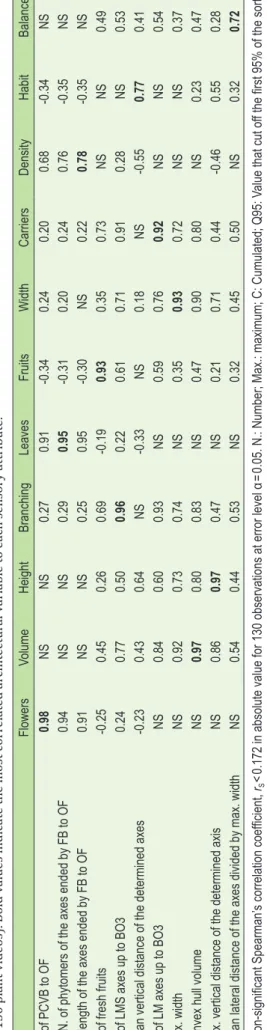
Table 5. Spearman corr elation matrix betw een sensory attribut es (columns) and respecti ve ar chit ectur al plant-scale variables (r ow
s) the most corr
elat ed ther et o f or the entir e dataset (N =130 pla nt videos). Bold v alues in dicat
e the most corr
elat ed ar chit ectur al v ariable t
o each sensory attribut
e. Flowers Volume Height Branching Leaves Fruits Width Carriers Density Habit Balance N. of PCVB to OF 0.98 NS NS 0.27 0.91 -0.34 0.24 0.20 0.68 -0.34 NS
C. N. of phytomers of the axes ended by FB to OF
0.94 NS NS 0.29 0.95 -0.31 0.20 0.24 0.76 -0.35 NS
C. length of the axes ended by FB to OF
0.91 NS NS 0.25 0.95 -0.30 NS 0.22 0.78 -0.35 NS N. of fresh fruits -0.25 0.45 0.26 0.69 -0.19 0.93 0.35 0.73 NS NS 0.49 N. of LMS axes up to BO3 0.24 0.77 0.50 0.96 0.22 0.61 0.71 0.91 0.28 NS 0.53
Mean vertical distance of the determined axes
-0.23 0.43 0.64 NS -0.33 NS 0.18 NS -0.55 0.77 0.41 N. of LM axes up to BO3 NS 0.84 0.60 0.93 NS 0.59 0.76 0.92 NS NS 0.54 Max. width NS 0.92 0.73 0.74 NS 0.35 0.93 0.72 NS NS 0.37
Convex hull volume
NS 0.97 0.80 0.83 NS 0.47 0.90 0.80 NS 0.23 0.47
Max. vertical distance of the determined axis
NS 0.86 0.97 0.47 NS 0.21 0.71 0.44 -0.46 0.55 0.28
Mean lateral distance of the axes divided by max. width
NS 0.54 0.44 0.53 NS 0.32 0.45 0.50 NS 0.32 0.72 NS: Non-significant Spearman’ s correlation coefficient, rS <0.172 in absolute value for 130 observations at error level α= 0.05. N.: Number; Max.: maximum; C: Cumulated; Q95: Value that cut off the first 95% of the sorted
values in ascending order
. FB: floral bud; PCVB: Petal Colour V
isible Bud; OF open flower
. L: long; M: Medium; S: Short. BO: Branching Order followed by the level, BO1 is the first branching order
V o l u m e 8 3 | I s s u e 3 | J u n e 2 0 1 8 197
Relating visual and architectural characterizations
Significant high to very high correlations were found for all the sensory attributes with at least one architectural plant-scale variable (Table 5). Very strong relations were found for the attributes assessing quantity and metric traits, the smallest Spearman’s correlation coefficient (rS) was 0.92 between
‘car-riers’ and the number of long and medium axes up to the third branching order; and the highest was 0.98 between ‘flowers’ and the number of floral buds with petal colour visible and open flowers. Lower but still high correlations, ranging from 0.72 to 0.78, were found for ‘balance’, ‘density’, and ‘habit’. While correlations of the architectural variables the most re-lated to ‘habit’ and ‘balance’ with the other attributes were in-deed lower, the cumulated length of the axes ended by a floral bud to an open flower was much more correlated to ‘flowers’ and ‘leaves’ than with ‘density’. Overall, similar correlations were found for the same attributes with different variables and on the opposite, especially with the variables related to ‘flowers’, ‘leaves’, and ‘density’; to ‘carriers’ and ‘branching’; then to ‘volume’, ‘width’, and ‘height’.
Correlations do not imply causations and may vary con-sidering the sub-samples studied. Thereby, cross-validation on calibration data and validation on unknown data under-taken using OLS models with predictor transformations en-abled the predictive efficiency of the available plant-scale architectural variables to be assessed more robustly. Table 6 summarizing the statistics of the models minimizing the pre-diction error with unknown data (RMSEP) showed that the most correlated architectural variables highlighted previous-ly were not necessariprevious-ly those leading to the best models, and that non-linear relationships were in most cases much more adapted. Overall, predictive abilities of the models obtained were quite remarkable especially for the sensory attributes related to metric and quantity traits. The less accurate model presented a relative error of prediction that did not exceed 17.3%, corresponding to the range normalized RMSEPof 1.09 for the attribute ‘balance’. Models with lesser perfor-mances in prediction were obtained for ‘density’, ‘habit’, and ‘balance’, suggesting potential links between panel perfor-mance for the sensory attributes and predictive abilities of the models that can be expected.
Discussion
Light modulation through shading enabled to induce phenotypic plasticity for the architecture of the ‘Radrazz’ rose bush. As already highlighted and especially exploited for the production of cut roses, results confirm the strong influ-ence of light on the rose architecture, especially for its initial signal role in the regulation and expression of the process related to organogenesis and branching. (Zieslin and Mor, 1990; Crespel et al., 2014; Leduc et al., 2014).
From ecological and botanical points of view, results strengthen observations made about the large phenotypic plasticity of shrubs, often in response to light gradients, en-abling them to adopt highly contrasted architectural devel-opment strategies according to local conditions (Valladares et al., 2000; Kawamura and Takeda, 2002, 2004; Pearcy et al., 2005; Charles-Dominique et al., 2010, 2012, 2015; Charles-Dominique, 2012; Sterck et al., 2013; Guzmán and Cordero, 2016).
This study allows to analyze the architecture of the ‘Radrazz’ rose bush and more broadly to provide information on the architectural development of shrubs throughout their life cycle. To resume the observed variability between axes and for predicting branching and carrying branch amounts, present results highlighted the relevance of the axis length based segmentation proposed, e.g., as used for apple tree architecture phenotyping and modeling (Costes et al., 2003; Pallas et al., 2016). Indeed, with age, delayed branching (pro-leptic), which is discernible by little scaly phytomers at the basis of the axes, is more and more prevalent within plants. The contrasted plants obtained with the shading experiment design, complementary results showed that this axis-length-based segmentation provided a quite stable pattern for the axis length distribution closely linked to branching orders within plants. Most of the basal sprouts leading to the archi-tectural systems here labeled as ‘delayed’ were carried by longer axes, well supporting the first part of the definition for reiteration summarized in Costes et al. (2014): a shoot with a comparable or longer length than its parent shoot and that partially or totally repeats the parental branching system. However, together with length, the orientation of the first branching order axes suggest quite different functions
Table 6. Predictive abilities of the OLS models minimizing the root error mean square error on validation test set (RMSEP)
to predict each sensory attribute.
Attribute Architectural variable PP
Model calibration1
n=90 plant videos n=40 plant videosModel validation R2
CV RMSECV Q2 RMSEP
Flowers N. of OF SR 0.97 ± 0.03 0.49 ± 0.19 0.95 0.53
Volume Convex hull volume CR 0.95 ± 0.02 0.40 ± 0.09 0.95 0.39
Height Max. vertical dist. of the determined axes YJ 0.95 ± 0.03 0.44 ± 0.09 0.93 0.46
Fruits N. of fresh fruits SR 0.95 ± 0.04 0.47 ± 0.13 0.91 0.63
Branching N. of LMS axes up to BO4 SR 0.93 ± 0.04 0.53 ± 0.12 0.94 0.47
Leaves C. length of the axes ended by FB to OF SR 0.92 ± 0.05 0.81 ± 0.24 0.96 0.49
Carriers N. of LM axes up to the BO3 Raw 0.83 ± 0.08 0.66 ± 0.14 0.89 0.49
Width Max. width (of the phytomer cloud) YJ 0.88 ± 0.08 0.50 ± 0.12 0.84 0.55
Habit Q95 vertical dist. divided by Q95 lateral dist. CR 0.63 ± 0.23 0.81 ± 0.18 0.66 0.80
Density N. of FB to OF SR 0.61 ± 0.20 1.11 ± 0.17 0.67 0.97
Balance Max. width divided by mean vertical distance C 0.54 ± 0.19 1.13 ± 0.22 0.49 1.09
1 Values are means ± standard deviations computed from 10 repeats of 10-fold cross-validation (CV). PP: Pre-processing transformation of the
architectural variables, YJ: Yeo-Johnson; SR: Square Root, CR: Cubic Root; C: Cube. N: Number; Max.: maximum; C: Cumulated; Q95: Value that cut off the first 95% of the sorted values in ascending order. FB: Floral Bud; OF: Open Flower. L: Long; M: Medium; S: Short. BO: Branching Order followed by the level, BO1: first branching order.
198 E u r o p e a n J o u r n a l o f H o r t i c u l t u r a l S c i e n c e and different profiles between shading conditions.
Support-ing the reiteration definition with respect to the architec-tural unit and its total reiteration concepts (Barthélémy and Caraglio, 2007), quite relevant for tree life cycle (Raimbault and Tanguy, 1993; Fay, 2002; Ishii et al., 2007), seems thus to present some inconsistencies for transposing the pattern and terminology used for trees to the rose bush and more generally to shrubs (Barthélémy and Caraglio, 2007; Y. Cara-glio and G. Galopin, pers. commun.). Indeed, to observe plain-ly the Champagnat model (Hallé et al., 1978; Costes et al., 2014), ‘Radrazz’ has to develop relay and renewal shoots, seen up to now as reiterated complexes, but quite different from the ‘elementary architectural structure stage’ (Crespel et al., 2013; Li-Marchetti et al., 2015) and its development. Nonetheless, by definition, total reiteration does not lead to newest axis categories and thus should not be integrated to define neither the architectural model, nor the architectural unit. Similar observations led to revisit the Tomlinson model for basitonic branching plants (Cremers and Edelin, 1995). We may ask if the reiteration process for shrub plants should be revisited or refined to integrate the hypothesis that this process may be necessary to the architectural unit construc-tion (‘establishement phase’, see Barthélémy and Caraglio, 2007) rather than a duplication of the first primary axis. Fu-ture analysis of the data using Hidden Markov chains Tree (HMT) model (Durand et al., 2005) together with similarity and distance indices between tree-structured data (Ferraro and Godin, 2000, 2003; Segura et al., 2008) to investigate finely the typology of the axes together with their topology and mutual matching may enable addressing more deeply such a hypothesis to further propose more relevant concepts for the life cycle pattern of shrubs forming bushes.
The study demonstrated the relevance of the method proposed for studying the relationships between plant ar-chitecture and main visual components. Video stands en-abled the avoidance of all possible product alteration during sensory tasks, especially critical for the state of the flowers. During panel formation, 17 sensory attributes were finally proposed. They were not all strictly similar but very close and coherent with the vocabulary and attributes highlighted for virtual ‘Radrazz’ rose bushes assessed using video (Gar-bez et al., 2015, 2016), or for real ones assessed directly or using unique plant facet photographs (Boumaza et al., 2009, 2010; Huché-Thélier et al., 2011; Santagostini et al., 2014). Among the 17 sensory attributes, the panel performance was good enough for 11 of them. Consensual attributes were related to plant size, plant shape, and quantification of the organs. The six other attributes not considered here are not uninteresting so far. They may be more suitable and relevant for studying other cultivars than ‘Radrazz’, or for experi-ments with other cultural practices. Besides, enhancing pan-el training with more precise protocol notation, definitions, and product references for the attributes and practice scaling test tasks with feedback for calibration is highly recommend-ed (Rainey, 1986; Wolters and Allchurch, 1994; Labbe et al., 2004; Findlay et al., 2007). Furthermore, multiple methods to present the stimuli may be investigated. For example, pre-senting organs ex-planta on static images as stimuli for as-sessing characteristics at the organ scale such as ‘leaf size’, or also ‘flower colour intensity’ or ‘flower size’ not investigated here, may be thus more efficient for the characterizations at the organs scale.
Finally, results obtained previously using virtual rose bush videos were confirmed with real plant material, with the validation of a protocol (number of videos, scoring
ses-sions, and number of subjects). The obtained models enabled us to identify architectural variables with good predictive ability and especially relevant for explaining the visual ap-pearance of the architecture of the rose bush. They reflected branching, growth and sexual expression of the axes as their structure in space, especially critical in the architectural es-tablishment of the rose bush. Such variables enabled here the characterization of the plants cultivated under three con-trasted shading environments with a reduced and coherent set of features over time. The large number of architectural variables that can be obtained, as here considering the meth-odological choice made, led to numerous comparable predic-tive models with quite acceptable results for each sensory at-tribute. Such results should thus lead researchers to carefully address the relevance of the variables selected from biologi-cal and practibiologi-cal viewpoints, and thus investigate more spe-cific analyses, merging expert knowledge and advanced sta-tistical methods adapted to variable selection and modeling under the ‘n<p’ conditions (Zucchini, 2000; Kuhn and John-son, 2013; Silva et al., 2013) as illustrated previously with virtual rose bush and predictive image analysis-based mod-els (Garbez et al., 2016). Upcoming analyses will address on the real plants the relevance of this previously tested image analysis method with more elaborated predictive modeling procedures, which may present relevant results, especially for sensory attributes concerning complex multidimensional visual traits, as here with the plant growth habit, its density and its balance. Improvements in the approach may concern image (size and resolution) and scene management for video editing in order to provide the most fitting plant visualiza-tion. Comparing results obtained from same plants present-ed using different stands is nevertheless necessary to gain more precise insights in the visual perception of ornamental plants.
Acknowledgments
The authors thank the Pays de la Loire Regional Council for their financial support; as the Pépinières Desmartis nursery and the National Association for Research and Technology (ANRT) for the Industrial Agreements for Research Training grant awarded (CIFRE grant number 2013/0410). The authors thank also Liu-Ji Harada for his investment during the data collection along his internship; all the people who took part in the sensory experiments; as Rémi Gardet and his team (INEM) from the Agrocampus Ouest Experimental Station for the crop monitoring support.
References
Abràmoff, M.D., Magalhães, P.J., and Ram, S.J. (2004). Image processing with ImageJ. Biophotonics Int. 11, 36–42.
Anchang, J.Y., Ananga, E.O., and Pu, R. (2016). An efficient unsupervised index based approach for mapping urban vegetation from IKONOS imagery. Int. J. Appl. Earth Observ. and Geoinform. 50, 211–220. https://doi.org/10.1016/j.jag.2016.04.001.
Barthélémy, D., and Caraglio, Y. (2007). Plant architecture: a dynamic, multilevel and comprehensive approach to plant form, structure and ontogeny. Annals of Botany 99, 375–407. https://doi.org/10.1093/ aob/mcl260.
Bates, D., Maechler, M., Bolker, B., and Walker, S. (2016). lme4: Linear mixed-effects models using ‘Eigen’ and S4. https://cran.r-project. org/package=lme4.
Bivand, R., Ono, H., Dunlap, R., and Stigler, M. (2015). classInt: Choose Univariate Class Intervals (Version 0.1–23). https://cran.r-project. org/package=classInt.