HAL Id: hal-03112604
https://hal.archives-ouvertes.fr/hal-03112604
Submitted on 17 Jan 2021
HAL is a multi-disciplinary open access
archive for the deposit and dissemination of
sci-entific research documents, whether they are
pub-lished or not. The documents may come from
teaching and research institutions in France or
abroad, or from public or private research centers.
L’archive ouverte pluridisciplinaire HAL, est
destinée au dépôt et à la diffusion de documents
scientifiques de niveau recherche, publiés ou non,
émanant des établissements d’enseignement et de
recherche français ou étrangers, des laboratoires
publics ou privés.
Sub meso scale phytoplankton distribution in the North
East Atlantic surface waters determined with an
automated flow cytometer
Melilotus Thyssen, N. Garcia, M. Denis
To cite this version:
Melilotus Thyssen, N. Garcia, M. Denis. Sub meso scale phytoplankton distribution in the North
East Atlantic surface waters determined with an automated flow cytometer. Biogeosciences, European
Geosciences Union, 2009, 6 (4), pp.569-583. �10.5194/bg-6-569-2009�. �hal-03112604�
www.biogeosciences.net/6/569/2009/
© Author(s) 2009. This work is distributed under the Creative Commons Attribution 3.0 License.
Biogeosciences
Sub meso scale phytoplankton distribution in the North East
Atlantic surface waters determined with an automated flow
cytometer
M. Thyssen, N. Garcia, and M. Denis
Laboratoire de Microbiologie, G´eochimie et Ecologie Marines, CNRS UMR 6117, Universit´e de la M´editerran´ee, Centre d’Oc´eanologie de Marseille, 163 avenue de Luminy, Case 901, 13288 Marseille cedex 09, France
Received: 22 April 2008 – Published in Biogeosciences Discuss.: 12 June 2008 Revised: 18 February 2009 – Accepted: 10 March 2009 – Published: 8 April 2009
Abstract. Phytoplankton cells in the size range ∼1–50 µm
were analysed in surface waters using an automated flow cy-tometer, the Cytosub (http://www.cytobuoy.com), from the Azores to the French Brittany during spring 2007. The Cy-tosub records the pulse shape of the optical signals gener-ated by phytoplankton cells when intercepted by the laser beam. A total of 6 distinct optical groups were resolved during the whole transect, and the high frequency sampling (15 min) provided evidence for the cellular cycle (based on cyclic changes in cell size and fluorescence) and distribution changes linked to the different water characteristics crossed in the North East Atlantic provinces. Nutrient concentrations and mixed layer depth varied from west to east, with a de-crease in the mixed layer depth and high nutrient concentra-tions in the middle of the transect as well as near the French coast. Data provided a link between the sub meso scale pro-cesses and phytoplankton patchiness, some abundance vari-ations due to the cellular cycle can be pointed out. The high frequency spatial sampling encompasses temporal variations of the phytoplankton abundance, offering a better insight into phytoplankton distribution.
1 Introduction
Phytoplankton encompasses thousands of species that de-velop by simple division at a rate of about once a day, thus potentially doubling their abundance every 24 h. The process is regulated by a succession of abiotic and biotic interactions specific to marine environments. The phytoplankton size range is spread over 4 orders of magnitude. From a recent
Correspondence to: M. Thyssen
(melilotus.thyssen@univmed.fr)
estimation, phytoplankton would represent 2% of the earth photosynthetic biomass, but they contribute to ∼45% of the earth annual primary production (Field et al., 1998). Pico-phytoplankton cells are the most abundant, particularly in the Oceanic oligotrophic provinces where their small size pro-vides them a better buoyancy and accessibility to nutrients. The abundance of nano- and microphytoplankton highly de-pends on nutrient availability, the increase of which occurs after the shoaling of the winter mixed layer in early spring for example. Phytoplankton can occasionally behave as an inert tracer, depending on the hydrodynamism of their envi-ronment (Skellam, 1951). However, the situation is not as simple. Indeed, the abundance variability of phytoplankton, composed of drifting cells, is not only controlled by division processes, but also by grazing, sinking, viral lysis, light and competition for nutrients, all depending on the scale and the strength of the surrounding physical processes (Fogg, 1991). This results in heterogeneous distributions with respect to both time and space, regarding abundances and assemblage composition. The actual phytoplankton data sets seldom re-group information on the spatial and temporal dynamics as well as on the morphological and physiological status of the studied entities. As a consequence, the categorisation and explanation of the observed patchiness highly depends on the definition of the sampling strategy and may be different from one study to another because of inadequate sampling frequencies (Sherry and Wood, 2001).
Phytoplankton spatial distributions are mathematically de-fined through spectral analysis (Gower et al., 1980), mul-tifractal processes (Seuront et al., 1996), wavelet analy-sis (Henson and Thomas, 2007) and multipoint correlation (Garcia-Moliner et al., 1993). The aim of mathematical treatments is to define the structure of the phytoplankton patchiness and their dependence on physical or biological
570 M. Thyssen et al.: North Atlantic phytoplankton high resolution
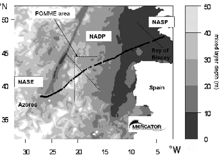
Fig. 1. Sampling area. The ship track is superimposed to the aver-aged mixed layer depth map from the 14 April to the 25 April 2007, derived from the MERCATOR model of the MERCATOR Ocean’s group. The main Provinces defined by Longhurst et al. (1995), and the POMME study area (Memery et al., 2005) are mentioned.
processes. They are running on data collected through telede-tection (estimation of chl-a concentration), automated fluo-rometry high frequency recording, spatial and temporal sam-pling involving pigment analysis and cell counts (either by flow cytometry or optical microscopy). These approaches need calibration of abundances and adjustment of temporal frequencies fitting biological processes in order to properly address in situ diversity and physiology status of the phyto-planktonic assemblages at sub meso scale to meso scale. It is important to accumulate as much information as possible on the origin and amplitude of the phytoplankton distribution variability in order to correctly define the processes that gov-ern the phytoplankton distribution and to better understand the marine ecosystem functioning.
The North Atlantic Ocean spring bloom is one of the most impressive when observing satellite images. This area is considered as a strong carbon sink (Takahashi et al., 2002), and the evolution of the North Atlantic bloom was subject to many studies (Ducklow and Harris 1993; Memery et al., 2005). Many processes can be involved in the origin, inten-sity and duration of the North Atlantic bloom (Siegel et al., 2002), and their characterisation requires a set of accurate methods in order to collect representative data. However, in situ observations in open waters covering both spatial and temporal scales of the phytoplankton dynamics and diversity are lacking.
In this paper, we describe the phytoplankton surface dis-tribution determined with an automated flow cytometer (Cy-tosub, Cytobuoy b.v.; Dubelaar et al., 1999; Thyssen et al., 2008a) during April 2007, at a sub meso scale sampling res-olution (1–10 km), in the North-East Atlantic Ocean, along a transect from the Azores Islands (Portugal) to the French Brittany. This instrument collects the pulse shape of each
optical parameter, enabling the cell discrimination into sim-ilar optical groups. Relationships were established between the different flow cytometric groups and the successive water characteristics crossed during the cruise and defined by their salinity, temperature and nutrient content. The access to the sub meso scale variability offers a high definition of infor-mation on the phytoplankton distribution, giving rise to the interpretation of its distribution.
2 Material and methods 2.1 Sampling strategy
Samples were automatically collected from 14 to 23 April 2007 during a cruise of the “Fetia Ura” sailing ship between Horta (38.6◦N–28.6◦W, Island of Fa¨ıal, Azores) and Lori-ent (47.6◦N–3.6◦W, French Brittany) (Fig. 1). Seawater was pumped from the ship central non toxic seawater supply (sit-uated in the centre of the boat) at 1.5 m depth every 15 min during 3 min at 30 dm3s−1, filling a 1 dm3reservoir sampled by the Cytosub 2 min after the pump stopped in order to let air bubbles disappear. The pump used the flexible impeller technology that does not squeeze the water passing through, avoiding the damaging of the cells.
Another reservoir containing a Conductivity, Temperature Depth (CTD, Microcat SBE 37) sensor was fixed on the deck and simultaneously filled in order to determine in parallel the temperature and the salinity of the seawater analysed by the Cytosub. The CTD was checked by the constructor before and after the cruise with no calibration needed.
2.2 The Cytosub
The Cytosub was designed to analyse large phytoplanktonic cells (1 to 1000 µm and a few mm in length) and relatively large water volumes (up to 4 cm3 per sample). It was ca-ble connected for energy supply and data transfer to a com-puter. The seawater was pumped to fill a sample loop be-fore entering the flow cell in order to avoid external turbu-lences and run the analysis at atmospheric pressure. The sample flow was controlled by a peristaltic pump working at a rate of 8.3 mm3s−1. The instrument used 0.2 µm fil-tered seawater containing ∼1% paraformaldehyde fixative as a sheath fluid. The sheath flow rate was 4800 cm3s−1. The sheath fluid and the analysed seawater were mixed together at the output of the flow cell and filtered through a 0.2 µm Polycap™ AS Nuclepore cartridge in order to be recycled. In the flow cell, each particle was intercepted by a laser beam (Coherent solid-state Sapphire, 488 nm, 15 mW) and the gen-erated optical signals were recorded. The light scattered at 90◦ (side scatter) and fluorescence signals were dispersed by a concave holographic grating and collected via a hybrid photomultiplier (HPMT). The forward scatter signal was col-lected via a PIN photodiode. The red (FLR), orange (FLO)
and yellow (FLY) fluorescences were collected in the wave-length ranges 668–734, 601–668 and 536–601 nm, respec-tively. Data recording was triggered by the forward scatter signal. The shape of the signals was encoded at a frequency of 4 MHz and data were saved in distinct 64 kbit grabbers before their transfer to a computer through the connecting cable. Particles flew at a rate of 2 m s−1through the 5 µm laser beam so that for instance the forward scatter signal shape of 1 µm beads would be defined by ∼12 points. More generally, particles flowing along their long axis (L (µm)), would have the shape of their forward scatter signal defined by 2*(5+L) points. The laser alignment and calibration pro-cesses were done before and after the cruise using Beckman Coulter Flow-count™ fluorospheres (10 µm).
2.3 Cytometric softwares
Cytoclus software (version 2004, Cytobuoy b.v.) was used to analyse the data collected by the Cytosub. Clusters were se-lected by taking into account the amplitude and the shape of the different signals. In addition to 5 average signal heights for forward scatter (FWS), sideward scatter (SWS) and for three fluorescence signals: red (FLR), orange (FLO) and yel-low (FLY), some simple mathematical models were assigned to each signal shape: inertia, fill factor, asymmetry, number of peaks, length and apparent size (FWS size) (Dubelaar et al., 2003). All these values are summarised in cytograms that facilitate the identification of clusters of cells sharing similar optical properties derived from those mathematical models. The boundaries of each cluster varied following diel cycles, and they were manually readjusted for each analysed sample.
2.4 Statistical analysis
Statistical analyses were performed on R freeware (http: //cran.r-project.org/). A non parametric local weighted poly-nomial regression calculation (Cleveland and Devlin, 1988) script (function LOESS) was applied to the signal of the cell abundances, their red fluorescence and their forward scatter dynamics in order to collect the smoothed signals. In order to collect the loess error, the data were bootstrapped 200 times before each loess calculation by re-sampling 90% of the data and re-evaluating the loess resulting signal. This provided an evaluation of the standard error of the initial loess calcu-lation applied to the raw data. The polynomial of order 2 was fit using weighted least squares, giving more weight to points near the point whose response is being estimated and less weight to points further away. A user-specific input to the loess calculation is possible, and is called “span”. The span determines how much of the data is used to fit each lo-cal polynomial. The span varies from 0 to 1; 0 resulting in a non smoothed signal. To extract the variability (low span) of the signals from the trends (high span), each low span boot-strapped loess calculations were subtracted from the high span bootstrapped loess calculation resulting in 200×200
differences. On those differences, the autocorrelation script (function ACF) was used, the average of the autocorrelations and the standard deviation were plotted in order to provide evidence of periodicities in the resulting data set by calculat-ing the correlation of the time series against a time-shifted version of itself. The two first absolute maximal significant autocorrelation values (average and standard deviation) were collected. The confidence interval of the ACF varied from 0.90 to 0.99 and was calculated depending on the number of samples used.
Spearman rank correlation calculations were used to make evidence of relations between cluster variables and hydrolog-ical values on the different water masses crossed.
2.5 Nutrients analysis
Nutrient (NO3−, NO2−, PO43−, Si(OH)
4) analyses were processed using 20 cm3seawater samples collected every 4 h from the 1 dm3 reservoir and transferred into polyethylene flasks directly frozen onboard. Analyses were performed us-ing a Technicon Autoanalyser® accordus-ing to Tr´eguer and LeCorre (1975). Detection limits were 50, 20, 20 and 50 nM for NO−3, NO−2, PO−4 and Si(OH)4, respectively.
2.6 Mixed layer depth estimation
The mixed layer depth was derived from the operational high resolution PSY2V2 model developed by the MERCATOR Ocean team (http://www.mercator-ocean.fr/). This model is based on the OPA8.1 primitive equations (Madec et al., 1998), specifically applied to the North Atlantic Ocean from 9◦N to 70◦N on a 1/15◦ horizontal Mercator grid
resolu-tion (5 to 7 km) and a 43 level vertical resoluresolu-tion (from 6 m up to 300 m). The PSY2V2 model is initiated from a sta-ble state using Reynaud’s climatology (Reynaud et al., 1998) and Smith et Sandwell’s bathymetry (Smith and Sandwell, 1997). Data input are retrieved once a week with in situ mea-surements (temperature and salinity profiles) from the Cori-olis data center, as for altimetry from remote sensing data. Sea surface temperature from remote sensing (1◦resolution) is used daily for assimilation. The configurations of the model are forced in real-time by daily fields of heat fluxes, fresh water fluxes, wind stress from the European Centre for Medium-Range Weather Forecasts (ECMWF) Numerical Weather Prediction system.
3 Results 3.1 Hydrology
A total of 691 samples were collected during the cruise. Average distance between successive samples was of 1.84±0.07 km. The ship track (Fig. 1) was superimposed on the map of the average mixed layer depth (MLD) as
572 M. Thyssen et al.: North Atlantic phytoplankton high resolution
Figure 2.
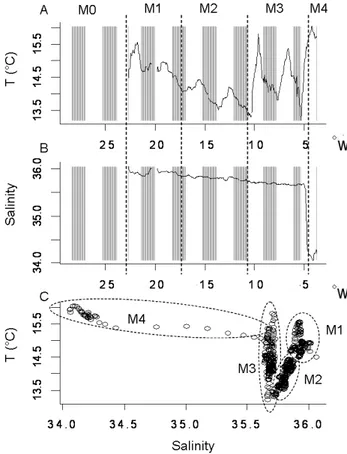
Fig. 2. Characteristics of the water types along the transect. (A) Surface temperature. (B) Surface salinity. (C) Temperature-Salinity plot resolving 4 distinct water types. Their location on the transect is indicated in panels (A) and (B).
calculated by the MERCATOR Ocean group between the 14– 25 April 2007.
Sea surface temperature ranged between 13.19 and 16.04◦C with an average value of 14.43±0.61◦C. Diel os-cillations were observable with a temperature decrease be-fore dusk. The maximum temperature variation between day and night was of 20% and occurred between the 21 and 23 April 2007 (between 10◦W and 5◦W, Fig. 2a). The min-imal temperature variation occurred within the period cov-ering the night of 17 April 2007 and the day of 18 April 2007 (between 21.20◦W and 18.5◦W, Fig. 2a). Salinity de-creased from the beginning of the CTD recording to the end (Fig. 2b). Values ranged between 34.05, near the French Brittany coast, and 36.05, in the North Atlantic open wa-ters. Average salinity was 35.07±0.38. No diel oscillation in salinity was detected but a small increase of salinity was observed between 20.65◦W and 19.45◦W, with an average value of 35.97, corresponding to the area with the lowest temperature diel variation, also characterised by a shallow mixed layer depth of about 10 m (MERCATOR Ocean). The cruise track crossed 4 water types labelled M1, M2, M3 and M4 and distinguished on the basis of their temperature and
Fig. 3. Nutrient distribution along the transect. (A) NO−3. (B) PO2−4 . (C) Si(OH)4. The location of the water types are
su-perimposed on the plots.
salinity features (Fig. 2c). Their average hydrological values and nutrient contents are reported in Table 1. The initial frac-tion of the track where temperature and salinity samples were unavailable was labelled M0. MERCATOR model data ob-tained day after day yielded MLD values of 20–50 m for M0 and M1. Deepest values were calculated inside of M1, reach-ing ∼50 m at 20.5◦W, with surrounding values of ∼25 m. In contrast, M2, M3 and M4 were characterised by shallower MLD, reaching ∼10 m depth (data not shown).
NO−3 concentrations varied from the detection limit up to 3.95 µM with an average value of 1.67±1.14 µM (Fig. 3a). The higher concentrations were observed within M1 and M2 and in the coastal waters M4 (Table 1). PO3−4 values var-ied between 0.07 and 0.42 µM with an average value of 0.2±0.08 µM (Fig. 3b). The highest concentrations were ob-served as well in M1, M2 and in M3 (Table 1). Redfield NO−3/PO3−4 ratio (Redfield, 1934) was <16 during the whole transect except near the French Brittany coast within M4, where it reached values of 30 (data not shown). Si(OH)4 concentrations ranged between 0.2 and 2.4 µM with an av-erage value of 1.05±0.4 µM (Fig. 3c) with an avav-erage value maximal inside M1 (Table 1). It is noteworthy that within M1 where diel temperature variations were the lowest, nutri-ent concnutri-entrations dropped down at about 21◦W, and partic-ularly that of Si(OH)4(Fig. 3).
Table 1. Water masses average characteristics, defined by their temperature-salinity properties (Fig. 2). Average values ± standard deviation
Temperature (◦C) Salinity (psu) NO3(µM) PO4(µM) SIOH4(µM)
Water masses M0 – – 0.61±0.26 0.14±0.03 1.18±0.17 M1 14.87±0.28 35.92±0.04 2.35±0.04 0.23±0.04 1.36±0.35 M2 13.93±0.29 35.80±0.04 2.62±0.50 0.28±0.05 1.15±0.47 M3 14.50±0.50 35.68±0.02 0.54±0.63 0.19±0.09 0.77±0.38 M4 15.67±0.25 34.39±0.45 3.15±0.72 0.11±0.04 0.52±0.41
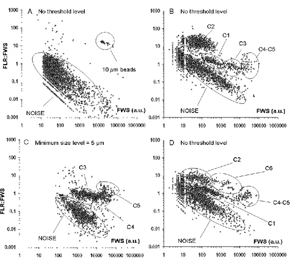
Fig. 4. Cytograms illustrating the cluster resolution. (A) FLR:FWS ratio (Red Fluorescence: Forward scatter) versus FWS for the analysis of 0.22 µm filtered seawater supplemented with 10 µm beads. No threshold level was applied so that the instrument noise could be recorded separately. (B) Same cytogram as in (A), related to the analysis of a pumped seawater sample. Four clusters were defined and labelled C1, C2, C3 and C4 (see Table 2 for the average values of their flow cytometric features). (C) Same cytogram as in (A) and (B) related to the analysis of a pumped seawater sample where a threshold was applied to the FWS signal in order to analyse a larger volume and address larger cells like those in C3, C4 and C5. (D) Same cytogram as in (B), illustrating the resolution of C6.
3.2 Cluster resolution
Six clusters were resolved over the whole transect as il-lustrated on Fig. 4b, c and d. Table 2 describes the average size and ratio (FLR/FLO and FWS/FLR) val-ues characterising the cells of each cluster as defined on
Fig. 4. Average cell length in the clusters varied from
<1 µm for C2 up to maximal values of 50 µm for the biggest cells within C5. C2 and C6 clusters exhibited FLR/FLO ratios approximately three times lower than those of the other clusters. Abundances were maximal for C1
574 M. Thyssen et al.: North Atlantic phytoplankton high resolution
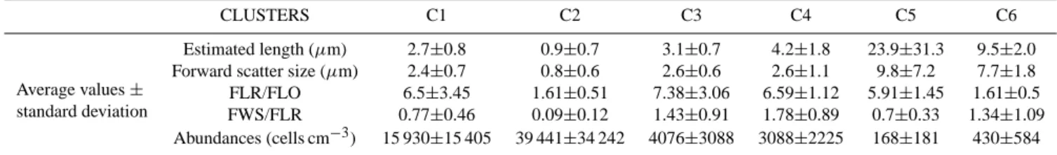
Table 2. Average values of cell abundances from the whole dataset and of flow cytometric parameters for the 6 resolved clusters. FLR:FLO is the red fluorescence (a.u.) on orange fluorescence (a.u.) ratio and FWS:FLR is the forward scatter (a.u.) on red fluorescence (a.u.) ratio. Due to the very high variability of the abundances, the standard deviation is larger than the average value which does not mean that abundances would be negative.
CLUSTERS C1 C2 C3 C4 C5 C6
Average values ±
Estimated length (µm) 2.7±0.8 0.9±0.7 3.1±0.7 4.2±1.8 23.9±31.3 9.5±2.0
standard deviation
Forward scatter size (µm) 2.4±0.7 0.8±0.6 2.6±0.6 2.6±1.1 9.8±7.2 7.7±1.8 FLR/FLO 6.5±3.45 1.61±0.51 7.38±3.06 6.59±1.12 5.91±1.45 1.61±0.5 FWS/FLR 0.77±0.46 0.09±0.12 1.43±0.91 1.78±0.89 0.7±0.33 1.34±1.09 Abundances (cells cm−3) 15 930±15 405 39 441±34 242 4076±3088 3088±2225 168±181 430±584
and C2 (average value 15.9×10³±15.4×10³cells cm−3and 39.4×10³±34.2×10³cells cm−3, respectively) and minimal for C5 (average value 168±181 cells cm−3).
3.3 Abundance, FLR and FWS spatial and temporal dynamics
The 6 defined clusters exhibited a high variability in abun-dance (Fig. 5), red fluorescence (Fig. 6) and forward scatter (Fig. 7) from the Azores up to the French Brittany. These figures were obtained by respectively plotting average abun-dance, FLR and FWS values per cell for each cluster over the whole transect. Open circles correspond to values averaged over 24 h successive periods.
C1 abundance increased from west to east, reach-ing maximal values of 110×103cells cm−3 in the east-ern part of M3 and inside M4 (Fig. 5a). C2 clus-ter exhibited two important abundance peaks, reaching
∼150×103cells cm−3 inside M0 (25.8◦W) and inside M2 (15.0◦W). Abundance values inside M1 were in average three times lower than in M2 (21.4×10³±7.8×10³ and 57.3×10³±46.9×10³cells cm−3, respectively) and twice lower in M3 (32.7×10³±14.8×10³cells cm−3) than in M2. C2 cluster was undetectable inside M4 (Fig. 5b). FWS and FLR of C2 cells exhibited a decrease through M0 but a sharp increase was observed before entering M1 waters. FLR average value kept decreasing be-tween M1 and the end of the transect (near 5◦W). Clus-ter C3 reached its maximal abundance inside M1 (aver-age value 8.3×10³±2.5×10³cells cm−3) and presented its lowest abundance values in both sampled coastal zones, more particularly near the French coast (average value inside M4 was 765.5±287 cells cm−3; Fig. 5c). Clus-ter C4 abundance had peaks inside M2, M3 and M4 (av-erage values: 3.9×10³±2.7×10³, 3.6×10³±2.4×10³ and 3.8×10³±2.4×10³cells cm−3 respectively; Fig. 5d). FLR (Fig. 6d) and particularly FWS (Fig. 7d) averaged values were lower inside M1 and M2 than elsewhere. C5 cluster was abundant near both coastal areas and particularly inside M4 (304±398 cells cm−3in M4 and 206±138 cells cm−3in
M0; Fig. 5e). FLR and FWS of C5 cluster were particu-larly high inside M2 (Figs. 6e and 7e). C6 cluster was essen-tially observed inside M2 and M3 (average values: 299±384 and 608±667 cells cm−3, respectively); it was nearly unde-tectable in M4 and remained below the detection level else-where (Fig. 5f).
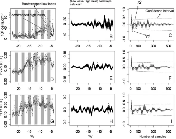
The short-term variability of abundance, FLR and FWS of the 6 clusters derived from loess treatments as detailed in Materials and Methods were submitted to autocorrelation calculations. Figure 8 illustrates such a data handling on abundance, FWS and FLR of cluster C1. In Fig. 8a, d and g are displayed the long-term trend and the weakly smoothed signal with their respective bootstrap variability. In Fig. 8b, e, and h are plotted the corresponding short-term variability obtained by subtracting all the bootstrapped long-term trends to all the bootstrapped weakly smoothed signals. Figure 8c, f and i illustrates the average autocorrelation calculations of the (short-term – long-term) bootstrapped differences and the standard deviations as well as the confidence interval of the autocorrelation function.
The two first maximal significant autocorrelation values and their standard deviation (first negative for r1 and first positive for r2) of the abundance, FWS and FLR short-term variability for the 6 clusters are reported in Table 3. The autocorrelation calculation for the C1 abundance short-term variability was with a lag of 13:30:00. Its FWS autocorre-lation calcuautocorre-lation was significant with a lag of 14:15:00 and only significant and negative for FLR at a lag of 06:15:00 (expressing half of a cycle of 12:30:00, Table 3). Conse-quently, abundance, FWS and FLR of C1 cluster varied cycli-cally twice a day, with an increase in the afternoon and in the early morning (Figs. 5a, 6a and 7a). The autocorrelation cal-culation for the C2 abundance, FWS and FLR yielded signif-icant values with lags of 20:45:00, 24:00:00 and 23:00:00 respectively (Table 3), expressing an approximately daily cycle for those three variables. Abundance variations pro-vided evidence for a second and shorter cycle of approx. 04:00:00 when the span used to define the difference between the general trend and the signal is sharper (span difference = 0.25–0.05, autocorrelation significant value=−0.32±0.11
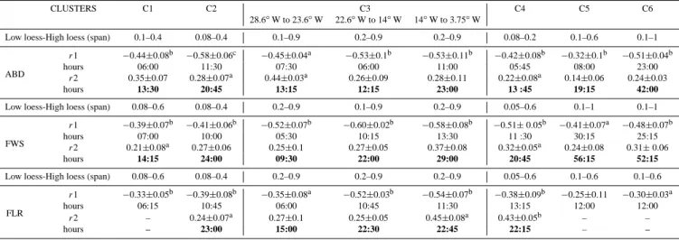
Table 3. Autocorrelation of the signal of abundances, FWS and FLR for each cluster obtained following the procedure illustrated on Fig. 8. The difference between the bootstrapped low loess and the bootstrapped high loess (the span level is user dependent) gives access to the small scale variability without the influence of the trend at a larger scale, and of the extreme values at a scale of successive samples. r1 and r2 are the two first negative and positive maximal significant autocorrelation values given at a sample lag corresponding to the hours.
CLUSTERS C1 C2 C3 C4 C5 C6
28.6◦W to 23.6◦W 22.6◦W to 14◦W 14◦W to 3.75◦W
Low loess-High loess (span) 0.1–0.4 0.08–0.4 0.1–0.9 0.2–0.9 0.2–0.9 0.08–0.2 0.1–0.6 0.1–1
ABD
r1 −0.44±0.08b −0.58±0.06c −0.45±0.04a −0.53±0.1b −0.53±0.11b −0.42±0.08b −0.32±0.1b −0.51±0.04b hours 06:00 11:30 07:30 06:00 11:00 05:45 08:00 23:00
r2 0.35±0.07 0.28±0.07a 0.44±0.03a 0.26±0.09 0.28±0.11 0.22±0.08a 0.14±0.06 0.24±0.03 hours 13:30 20:45 13:15 12:15 23:00 13 :45 19:15 42:00
Low loess-High loess (span) 0.08–0.6 0.08–0.4 0.2–0.9 0.1–0.9 0.2–0.9 0.05–0.6 0.1–1 0.1–1
FWS
r1 −0.39±0.07b −0.41±0.06b −0.52±0.07b −0.60±0.02b −0.58±0.08b −0.51± 0.05b −0.41±0.07a −0.48±0.07b hours 07:00 10:00 05:30 10:15 13:30 11 :30 30:15 25:15
r2 0.21±0.08a 0.27±0.06 0.25±0.1 0.27±0.05 0.37±0.08 0.32±0.05a 0.24±0.08 0.31± 0.06 hours 14:15 24:00 09:30 22:00 29:00 20:45 56:15 52:15
Low loess-High loess (span) 0.08–0.6 0.08–0.4 0.2–0.9 0.2–0.9 0.2–0.9 0.05–0.6 0.1–0.6 0.1–0.6
FLR r1 −0.33±0.05b −0.39±0.08b −0.35±0.08a −0.52±0.03b −0.54±0.07b −0.38±0.09b −0.25±0.11 −0.30±0.03a hours 06:15 10:45 06:00 10:45 11:30 13:15 12:00 12:00 r2 – 0.24±0.07a 0.27±0.1 0.25±0.05 0.45±0.08a 0.43±0.05b – – hours – 23:00 15:00 22:30 22:45 22:15 – – a: p<=0.1,b: p<=0.05,c: p<=0.01
Fig. 5. Distribution of cell abundances for each resolved cluster along the ship track. White dots are the daily average values of abundances. Day and night periods are indicated with white and grey boxes respectively. The different water types are specified on top of each plot.
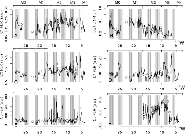
576 M. Thyssen et al.: North Atlantic phytoplankton high resolution
Fig. 6. Spatial variation along the ship track of the cell average red fluorescence (FLR) for each cluster. White dots are the daily average values of the cell average FLR. Day and night periods are indicated with white and grey boxes respectively. The different water types are specified on top of each plot.
(confidence interval=0.95) with a lag of 04:15:00 followed by −0.34±0.07 (confidence interval=0.99) with a lag of 11:30:00, which corresponds to the main signal as defined in Table 3), FWS and FLR autocorrelations did not show a shorter cycle. But at ∼10◦W, C2’s FLR and FWS increase occurred during the day, and not in the early evening as in M1 and M2.
Considering values averaged over 24 h successive peri-ods, FLR of C3 cluster was rather stable (Fig. 6c) whereas FWS increased along the transect (Fig. 7c). The cycle fre-quency of those parameters varied during the cruise. From the departure up to 23.6◦W, autocorrelations of abundance, FWS and FLR showed anti-autocorrelation significant sig-natures with lags of 07:30:00, 05:30:00 and 06:00:00, re-spectively (Table 3). Between 22.6◦W and 14◦W, anti-autocorrelations were significant with lags of 06:00:00, 10:15:00 and 10:45:00, respectively, indicating that abun-dance periodic variation had a frequency twice that of FWS and FLR. Between 14◦W and 3.75◦W, anti-autocorrelation values of the abundance, FWS and FLR were significant with nearly the same lags (11:00:00, 13:30:00 and 11:30:00, re-spectively).
Autocorrelation calculation supported significant periodic properties for C4 abundance, FWS and FLR with lags of 13:40:00, 20:45:00 and 22:15:00, respectively (Table 3). As
for C3, FLR and FWS expressed a diel periodicity whereas the abundance periodicity was twice a day, this peculiarity being maintained over the whole transect.
Autocorrelation calculations provided evidence of a pe-riodicity for C5 cluster abundance and FWS with a lag of 19:15:00 and a lag of 52:15:00, regarding the significant val-ues of the anti-autocorrelation results (Table 3) but failed for FLR.
C6 cells, although only observed in M2, M3 and M4, ex-pressed a 52:00:00 periodicity for their FWS signature and a 42:00:00 for their abundances and no significant autocorrela-tion value for their FLR variability.
3.4 Clusters dynamics: correlation with hydrological data
The relations between population and hydrology were evi-denced by correlating the cluster abundances, their FLR and their FWS with nutrients, temperature and salinity data and summarised in Table 4. Only water masses M1, M2 and M3 were used in those correlation calculations since the M0 and M4 waters were highly variable, generating a decrease in the overall correlations obtained. At the water mass scale, only a few variables were correlated together, that will be men-tioned further on a manuscript mode.
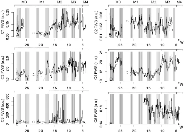
Fig. 7. Spatial variation along the ship track of the cell average forward scatter (FWS) for each cluster. White dots are the daily average values of the cell average FWS. Day and night periods are indicated with white and grey boxes respectively. The different water types crossed are specified on top of each plot.
Table 4. Spearman rank correlation values between the signal of abundance, FWS and FLR for each cluster and hydrological information (nitrate (µM), phosphate (µM), temperature (◦C) and salinity) inside water masses M1+M2+M3. Similar correlations inside each water mass between the selected variables are described in the Results section.
CLUSTERS C1 C2 C3 C4 C5 C6
M1+M2+M3 ABD FLR FWS ABD FLR FWS ABD FLR FWS ABD FLR FWS ABD FLR FWS ABD FLR FWS
NO3 n=46 −0.35a −0.23 −0.4b 0.30 0.35 −0.03 0.27 0.21 −0.24 −0.16 0.11 −0.50c −0.63c 0.02 −0.16 0.17 0.31 0.33
PO4 n=46 0.06 0.19 0.11 0.41b 0.07 −0.20 0.05 0.19 −0.23 −0.03 0.17 −0.31a −0.32 0.27 0.19 0.34 −0.04 0.05
Temperature n=555 0.09 −0.43c −0.36c −0.22 0.33c 0.44c 0.24 −0.53c −0.24 −0.08 −0.08 0.32c 0.08 −0.21 −0.08 −0.28c 0.02 −0.11
Salinity n=555 −0.6c −0.45c −0.77c −0.18 0.84c 0.28c 0.78c −0.1 −0.50c −0.06 −0.05 −0.52c −0.44c −0.09 −0.33c 0.06 −0.02 0.39c
a: p<=0.1,b: p<=0.05,c: p<=0.01
On a large scale (considering M1, M2 and M3), C1 abun-dance was anti-correlated to NO−3 and to salinity, C1 FLR to temperature and salinity and C1 FWS to temperature, salinity and NO−3 (Table 4). At the water mass scale, C1 abundance was correlated to PO3−4 and temperature (r=0.56, p<0.1,
n=4 and r=0.53, p<0.01, n=35, respectively) and anti-correlated to salinity (r=−0.54, p<0.01, n=35) in M4. C1 FLR was correlated to NO−3 inside of M0 (r=0.89, p<0.01,
n=11) and to PO3−4 inside of M3 (r=0.54, p<0.1, n=12). C1 FWS was anti-correlated to NO−3 inside of M3 (r=−0.81,
p<0.01, n=12).
C2 abundance was positively correlated to PO3−4 , C2 FLR and C2 FWS were positively correlated to temperature and salinity (Table 4). At the water mass scale, C2 abundance was anti-correlated to PO3−4 inside of M1 and correlated in-side of M2 (r=−0.75, p<0.1, n=9 and r=0.54, p<0.1, n=12, respectively). Inside of M3, C2 FLR and FWS were anti-correlated to PO3−4 (r=−0.58, p<0.1, n=12, and r=−0.77,
p<0.05, n=12, respectively).
C3 abundance was positively correlated with salinity; C3 FLR was negatively correlated with temperature and C3 FWS with salinity (Table 4). At the water mass scale, C3 abundance was anti-correlated to NO−3 in M1 (r=−0.71,
578 Figure 8. M. Thyssen et al.: North Atlantic phytoplankton high resolution
Fig. 8. Illustration of the procedure to get the autocorrelation values r1 and r2 and their corresponding standard deviation values using C1 cluster mentioned in Table 3. (A), (D) and (G) Superimposition of a bootstrapped high loess process and a bootstrapped low loess process calculated on the original data for (A) Abundance, (D) FLR and (C) FWS. Dots: Original data. Dashed lines: bootstrap of the smoothed data. Continuous lines: smoothed data. The spans used to define the high and the low loess are mentioned in Table 3. (B), (E) and (H) Difference of both loess bootstrap calculations in order to extract the short scale variability (low loess process) from the overall trend (high loess process). (C), (F) and (I) Average and standard deviation of the autocorrelation of all the signals illustrated in (B), (E) and (H). r1 and r2 are the two maximal significant values. Dashed line: confidence interval (p=0.1) of the autocorrelation.
p<0.1, n=9). C3 FLR was correlated to PO3−4 in M0 (r=0.56, p<0.1, n=11), anti-correlated to temperature in M2 (r=−0.78, p<0.01, n=222) and correlated to PO3−4 in M3 (r=0.77, p<0.01, n=12). C3 FWS was anti-correlated to salinity in M2 (r=−0.52, p<0.01, n=222).
C4 FWS was negatively correlated with nutrient concen-trations and salinity and positively with temperature (Ta-ble 4). At the water mass scale, C4 abundance was correlated to temperature and anti correlated to salinity in M4 (r=0.61,
p<0.01, n=35 and r=−0.53, p<0.01, n=35, respectively). C4 FLR was correlated to NO−3 and PO3−4 in M3 (r=0.66 and r=0.68, p<0.05, n=12). In M4, C4 FLR was corre-lated to temperature and anti-correcorre-lated to salinity (r=0.44 and r=−0.42, respectively, p<0.01, n=35). C4 FWS was correlated to NO−3 in M2 (r=0.57, p<0.05, n=12).
C5 abundance was positively correlated to NO−3 and neg-atively to salinity. C5 FWS had a negative correlation with salinity (Table 4). At the water mass scale, C5 abundance was anti-correlated to NO−3 and PO3−4 in M1 (r=−0.71 and
r=−0.79, p<0.1, n=9), correlated to temperature and anti-correlated to salinity in M4 (r=0.58 and r=−0.51, respectiv-elly, p<0.01, n=35). C5 FLR was anti-correlated to NO−3 in M1 (r=−0.71, p<0.1, n=11). C5 FWS was correlated to NO−3 in M1 and to PO3−4 in M2 (r=0.57, p<0.01, n=11 and
r=0.64, p<0.05, n=12, respectively).
C6 abundances were negatively correlated with temper-ature and C6 FWS was positively correlated with salinity (Table 4). At the water mass scale, C6 abundance was anti-correlated to NO−3 in M2, and correlated in M3 and M4 (r=−0.83, p<0.01, n=12, r=0.63, p<0.01, n=12 and
r=0.68, p<0.05, n=4, respectively). C6 FLR was corre-lated to NO−3 in M2 and M3 and to salinity in M3 (r=0.55,
p<0.1, n=12, r=0.80, p<0.01, n=12 and r=0.66, p<0.01,
n=166, respectively). C6 FWS was correlated to NO−3 in M3 (r=0.73, p<0.01, n=12).
4 Discussion
4.1 Hydrological background
The cruise track crossed three Atlantic provinces (Longhurst et al., 1995): (i) the North Atlantic East Province SubTropi-cal Gyre from the Azores to approximately 17–18◦W, corre-sponding to M0 and M1 water type areas; (ii) the North At-lantic Drift Province up to approximately 5◦W, correspond-ing to M2 and M3 water type areas; and (iii) the North At-lantic Shelves Provinces, corresponding to M4 water type area.
A strong southward geostrophic current was observed be-tween 40◦N–45◦N at 24◦W by Paillet and Mercier (1997),
generating a permanent frontal area more specifically lo-cated by Paillet and Arhan (1996) at 41–42◦N. This frontal
area may correspond to the one observed in 2001 during the spring POMME experiment (Fernandez et al., 2005). The in-crease of NO−3 observed between M0 and M1 is reminiscent of the one reported by Fernandez et al. (2005) who found during spring, low surface nutrient values (∼1 µM) south of this front and high values (close to 7 µM) north of it. Siegel et al. (2002), described two regimes north and south of 40◦N explaining the origin and the intensity of the phytoplankton bloom. South of this area, the bloom is theoretically limited by light but also by the nutrient availability which is linked to the intensity of the winter mixing, while in the north the bloom development depends on the achievement of the Sver-drup’s critical depth, which is mainly a light accessibility process.
4.2 Cluster resolution
The automated resolution of 6 clusters was made possible by recording the shape of 5 optical parameters giving access to the cell morphological variability (Jonker, 1995; Dube-laar and Gerritzen, 2000). The high sampling frequency and the permanent features of the observed clusters increased the accuracy of the method even if for less populated clusters, the direct counts were not always complying with the 3% tolerated variability (Thyssen et al., 2008a). The 6 clusters were nearly the same as those observed in previous studies (M. Zubkov, personal communication) as it is the case for ultraphytoplankton clusters definition using bench top flow cytometers. The average cell size in the observed clusters ranged from less than ∼1 µm up to 50 µm.
C1 cells corresponded in terms of size (∼2–3 µm, Table 2) to the picoeukaryote community whose average abundance value was 15.9±15.4×10³cells cm−3(Table 2). In the study of Zubkov et al. (2000), the abundance of picoeukaryote phy-toplankton varied from ∼10×103 to ∼15×103cells cm−3 with a peak of ∼25×103cells cm−3 at 50◦N. During 2001 POMME spring study (18◦W, 38–44◦N), surface values var-ied between ∼10×103and ∼50×103cells cm−3(Fernandez et al., 2007). In spring 2004, picoeukaryiote-phytoplankton
abundance peaked (∼14×103cells cm−3)in the North At-lantic East Province at 40◦N and made a major fraction of
to-tal phytoplankton in terms of abundance (Tarran et al., 2006). C2 cells had a strong orange fluorescence signature (Table 2) and their small size makes them looking like some phycoerythrin-containing picocyanobacteria (Sherry and Wood, 2001) such as Synechococcus. The abundance of C2 cells during this study matches the observed
Synechococ-cus abundances reported for surface samples collected from
22 April to 26 May 1997 in the North Atlantic between 35 and 45◦N: ∼20×103to 200×103cells cm−3(Zubkov et al., 2000; Fig. 5b).
The sum of all the other largest cells (C3, C4, C5 and C6) reached averaged values of 6.9×10³±4.3×10³cells cm−3, in between the surface abundance (14×103cells cm−3, un-published data) of nanoeukaryotes in spring 2001 within the POMME study area (18◦W, 38–44◦N), and surface abundances (max 2.2×10³cells cm−3)of nanoeukaryotes in spring 2004 (Tarran et al., 2006). In terms of biomass, Dan-donneau et al. (2004) reported that in the North Atlantic Drift Province, most of the phytoplankton was composed of nanoplankton (more than 70% of the biomass even during the spring bloom) and of microplankton (30–50% during April 2000 and April 2001).
4.3 Cluster dynamics
The cluster dynamics involved two different spatial scales: (i) the meso scale corresponding to water mass changes, and (ii) the sub meso scale at which cluster dynamics may have been driven by small physical processes under the strong in-fluence of the cell cycle occurring at a daily scale (time for the ship to cover about 150 km). The amplitude of tempera-ture and nutrient concentration variations was high at the sub meso scale, while salinity depicted less heterogeneity, giving insight to meso scale variations, apart from specific sub meso scale features that can modify salinity at a larger extent than the surrounding average.
The sub meso scale (1–10 km), where space and time are strongly linked, approximately corresponded to 1 to 4 sam-ples, or 15 min. to 1 h at the average speed of the ship. At this scale, clusters exhibited strong cell cycle signatures through FLR and FWS parameters, evidenced on their abundance dy-namics and clearly confirmed by the autocorrelation calcu-lation, as observed during a previous study in a Mediter-ranean harbour (Thyssen et al., 2008b). Abundance vari-ations, FLR and FWS diel variability were consistent with cell cycle in numerous studies (Jacquet et al., 2002; Binder and Durand, 2002, and references therein). During the whole study, the cell abundances were affected by the stage of the cell cycle at which sampling occurred. The cell cycle seemed to play a great role in the patchiness observed at sub meso scale. The other patchiness sources would be linked to other small spatial and temporal control factors such as interrelation between species, grazing, viral lysis, migration
580 M. Thyssen et al.: North Atlantic phytoplankton high resolution and turbulence. Considering meso scale, the distribution
of the clusters, the cell pigment content and cell size (FLR and FWS, respectively) varied with water properties. When addressing the spatial distribution of phytoplankton assem-blages at sub meso scale, it seems quite impossible to define a sampling frequency shorter than the smallest cell cycle that may lead to a correct representation of this distribution.
Cells in C1 cluster were about 2.5 µm in size and their FLR average value was 5 times lower than that of cells in C3 cluster in spite of their similar size (Table 2). Cells of C1 cluster divided approximately twice a day and most of the observed abundance peaks were consistent with this rate. The correlation between abundances and salinity in Table 4 is the expression of a meso scale relation, C1 abundances in-creasing while reaching the French coast. But this does not give information on the role of hydrology in C1 abundance distribution at the sub meso scale. On the same way, the vari-ation of the global FWS and FLR signals was linked to the crossed water types, as illustrated by the correlations with salinity (Table 4). On the other hand, the negative correla-tion with temperature, although weak (Table 4), suggests a link between daily variations of temperature and daily vari-ations of cellular activity, occurring at a sub meso scale, but since no correlation was observed at the water mass scale, no conclusion about temperature relation with C1 cells can be made. The decrease of FWS and FLR inside M1 can be related to a photoperiod decrease resulting from strong verti-cal mixing while consistently, the extent of the diel tempera-ture variations was low compared to that observed in M3 and M4. However, it seems that the cell cycle was not affected by vertical mixing, in agreement with Jacquet et al. (2002) who reported that strong physical perturbations did not mod-ify the picoeukaryote flow cytometric FLR signature of the cell cycle. Daily average C1 abundance was maximal inside M3 (Fig. 5b, open circles), corresponding to low nutrient val-ues (mainly NO−3, Fig. 3a), and minimal inside M1 and M2 where nutrients and certainly turbulence were high. Indeed, the mixed layer depth was still deep at those latitudes com-pare to northern areas of the North East Atlantic (Fig. 1). In addition, the intensity of winter mixing south of 40◦N, part of the North Atlantic East Province SubTropical Gyre, is the main source of nutrient input in surface waters by the advec-tion of deep and nutrient rich waters (Siegel et al., 2002) as observed for M1 and M2. C1 cells were more abundant in areas with low nutrient content (or non turbulent waters, Ta-ble 3) as commonly observed for picoeukaryotic cells, which was not the case for C2, C3 and C6 cells (Fig. 5b, c, f). But, C1 abundances were low inside M0 with relative low nutri-ent concnutri-entrations, and high in M4 with relative high nutrinutri-ent concentrations, suggesting that nutrients were not the princi-pal abundance regulation factor.
Following Nyquist sample theory (Nyquist, 1928) who defined the minimal sampling frequency of a system to be at least twice its highest frequency, in order to sample C1 cells correctly, it would be necessary to make one sample
at least every 6 h, or at the average speed of the boat, every 43.2 km. Anyway, this sampling distance may not resolve the sub meso scale processes that would require a higher sam-pling frequency.
Cells of C2 cluster were about 1 µm in size and were char-acterised by high orange fluorescence (FLO). Their abun-dance was maximal inside of M0 and of M2 and they were not detected near the French coast (Fig. 5b). Such a strong variation in abundance was reported by Martin et al. (2005) for Synechococcus cells, with a 50 fold increase 12 km apart. The diel cycle of cells belonging to C2 was similar to the one observed for Synechococcus in the North Atlantic Ocean (Olson et al., 1990; Wyman, 1999) and the north-western Mediterranean Sea (Jacquet et al., 2002), with an increase of FWS and FLR in the early evening leading to night division. However, the diel cycle of C2 cells seemed to shift between M2 and M3. Indeed, despite the strong autocorrelation of abundance, FLR and FWS (Table 3), the period during which FWS and FLR increased changed inside of M3. The diel cy-cle remained similar, but occurred earlier (maximum FLR and FWS during daylight), meaning that C2 cells were not synchronous over the track covered by the ship. Such a phase shift was observed for Synechococcus in the surface waters of the equatorial Pacific Ocean (Vaulot and Marie, 1999). The autocorrelation value of abundance dynamics was maximal at 20:45:00, very close to the 18:00:00–19:00:00 periodic-ity calculated for Synechococcus by using Fourrier analysis (Jacquet et al., 2002). M0 appeared as a peculiar environ-ment since a broad peak of abundance was observed during daytime, in contrast with the main peak of abundance inside M2 that occurred during night-time, just after the assumed cell division, and no specific FLR or FWS decrease were observed (Fig. 5). In parallel, FLR and FWS values of C2 cells were the lowest in M0 during daytime. Would C2 cells be represented by Synechococcus species, their photoprotec-tion properties (Vaulot and Marie, 1999) could not account for the large FLR decrease during daytime in M0 since the large mixed layer depth of M0 implies a rather low exposure to maximum light. Such a decrease in FLR and FWS did not occur so dramatically for the other clusters (Figs. 6 and 7). Jacquet et al. (2002) reported that an increase in pigment content for Synechoccocus could be linked to an increase in nutrient concentrations. In this study, a nutrient increase oc-curred inside M1 but FLR of C2 cells increased nearly 24 h before the ship entered M1. From M1 to M4, the daily aver-aged FLR decreased continuously, in correlation with salin-ity (Table 3) which may be explained by a change in compo-sition or in phenotype of the phycoerythrin-containing pico-cyanobacteria as observed in many cases for Synechococcus when reaching coastal zones (Wood et al., 1998). Daily cy-cle of FWS and FLR are positively correlated to temperature daily variations (Table 3), and as for C1, it suggests a link between temperature, physical processes and physiological cellular cycles at the sub meso scale. FLR correlations with salinity were high, suggesting a meso scale impact on the
decrease of the FLR while reaching the French coast. But, as for C1, no correlation was evidenced with our data at the scale of the water mass, limiting the conclusion about a hy-drological control of C2 cluster abundance variation.
Cells of C3 cluster exhibited a high periodicity with an abundance increase twice as fast as the FLR and FWS sig-natures up to the middle of M2 waters (i.e. 14◦W, Table 3). This may be linked to thermal water mass advection occur-ring between day and night, with no effect on cell cycle. In-deed, M1 may be the most dynamic area since the ship track may have crossed the north east frontal region as discussed previously. Around 41◦N–21◦W where C3 cells were the most concentrated, the MLD went from deep to shallow within a small distance (Fig. 1), and nutrient concentration showed a little decrease (Fig. 3). The C3 phytoplankton cells seemed to be under favourable development despite the lit-tle nutrient depletion, and salinity signature suggests that we may have crossed an eddy at a specific stage of the North Atlantic bloom evolution (Karrash et al., 1996; Garc¸on et al., 2001; Fernandez et al., 2005). The periodic variation of FLR and FWS increased in M1 and M2 with respect to M0 (from 09:30:00 and 15:00:00, respectively, in M0 to 22:00:00 and 22:30:00 in M1 and the first part of M2, Table 3), as for the daily average FLR and FWS amplitude (Figs. 6c and 7c) suggesting that in some favourable areas, the cells maintain high abundances with a small size and a low pigment con-tent, coupled to a decrease in growth rate. In the Bay of Bis-cay (Fig. 1), C3 abundance decreased but remained strongly influenced by the cell cycle as suggested by the frequency of FLR and FWS peaks that occurred with some delay with respect to the peak of abundance (Figs. 5c, 6c and 7c, Ta-ble 3). The negative correlation between FLR and tempera-ture make evidence of the increase of pigment contents dur-ing the night, when temperature decreases. This relation is evidenced inside of M2 by a high anti-correlation between FLR and temperature; at this place, the periodic variation of FLR and FWS reached a daily cycle. The FWS and the abun-dances of C3 were correlated to salinity, suggesting a meso scale influence on a global view.
C4 cells belonged to small nanoplankton (4 µm, Table 2); their FLR and FWS decreased in M1 and M2 (Figs. 6d and 7d) that may be related to the mixing processes as observed for C1 and C3 but lasting much longer for C4 cells since the increase in daily averaged FLR and FWS only occurred in-side M3, where correlations between those parameters and nutrient content were high. C4 abundance dynamics clearly illustrate the difference in information brought by high and low frequency sampling. The periodicity of C4 abundance was twice as fast as the assumed cell cycle derived from the FLR and FWS cyclic signatures (Table 3). In addition, the amplitude of the abundance cyclic variation increased up to 4 times inside M2 and M3, without affecting the average daily value (Fig. 5d). This may result from different biological parameters such as diel vertical migration, cyclic grazing or cyclic virus lysis that would have affected C4 cells during
the whole cruise, but not C3 cells. Furthermore, no correla-tion was evidenced with our data set between C4 abundance and hydrological variables at the water mass scale, but only for FWS at a large scale, suggesting a meso scale impact on C4 size. C4 cluster dynamics would have been impossible to describe if the sampling frequency were not appropriate to the specific abundance cycle of approx. 14:00:00. Following Nyquist theory (Nyquist, 1928), the maximum sampling in-terval to account for the C4 abundance periodicity would be 07:00:00, still too large to account for an accurate sub meso scale observation.
C5 cells were mostly present near the coasts (Fig. 5e) and their larger size implies a strong morphological diversity. High FLR and FWS signals (Figs. 6e and 7e) were observed inside M2 although C5 cell abundance was weak (around 100 cells cm−3), suggesting a cluster composition different from the one near the coasts rather than some physiological variation. This cluster was anti-correlated to nutrient, mostly inside of M1, and correlated to temperature inside of M4, giving little information on the hydrological impact on C5 abundance dynamics.
The abundance of C6 cells, characterised by a high FLO signal like C2 cells, varied periodically between the detec-tion limit and 2×10³cells cm−3. The abundance of C6 cells together with their FLR sharply decreased near the French coast but was elevated inside M2 like the abundance of C2 cells. In M2, C6 abundance was anti-correlated to nitrate concentration, but correlated in M3 and M4.
At the global Ocean scale, north of 40◦N, the develop-ment of the North Atlantic spring bloom goes northward, following the establishment of the Swerdrup’s critical depth (Swerdrup, 1953). However, south of 40◦N, its development
depends on nutrient availability linked to the winter mixed layer depth (Siegel et al., 2002). At the meso scale level, the situation appears less simple. Indeed, Karrasch et al. (1996) observed that the North Atlantic bloom formed a patchwork representing different development stages within meso scale features that may be over or under estimated due to a lack in sub meso scale observations.
In our study, we observed a series of different cell groups, each composed of similar cell morphotypes, depending on the crossed water types. M0 waters were part of the north-ern area of the North Atlantic Subtropical East Gyre, mostly oligotrophic. Abundances were generally low but C5 cells were more abundant in M0 than in the middle of the tran-sect. C3 cells appeared the most adapted to highly turbulent areas such as M1 waters that were on the edge of the two North East Atlantic Provinces. However, the maximum con-centration for C3 cells was observed within a specific area inside M1 that could be reminiscent of some isolated eddy interior. In the northward adjacent M2 water type, C2 and C4 cells were at their highest abundances. The Bay of Bis-cay waters (M3) were certainly at an advanced stage of the North Atlantic bloom, with a shallow mixed layer depth and low nutrient concentrations. Those waters were particularly
582 M. Thyssen et al.: North Atlantic phytoplankton high resolution suited for C1 small cells, C4, C5 and C6 cells. Abundances
reached high values as observed for previous spring blooms (Tarran et al., 2006). M4 coastal waters were specifically rich in NO−3, favouring the large C5 cells, but also C1 and C3 cells. It is difficult to make evidence of spatial or tem-poral processes in abundance variations; cellular cycle may only explain one part of the abundance variations. But since no similar abundance variation between the different clusters was observed, it is difficult to imagine one strong physical influence, such as aggregation or dispersion phenomenon, at the meso scale or at the sub meso scale. Those spatial and physical phenomenons may be true for larger cells that do not present such high division rates, and such high concen-trations.
5 Conclusion
The automated high frequency sampling conducted with the Cytosub from the Azores up to the French Brittany during April 2007 singled out the importance of a high frequency sampling, both in space and time, in agreement with the flu-orometry study of Rantajarvi et al. (1998). Sub meso scale processes are certainly affected by micro scale processes. Modelling phytoplankton distribution in the marine ecosys-tem is better achieved by considering its sub meso scale than its meso scale distribution, because the sub meso scale distri-bution takes into account the natural cell cycle. Thus, the cell cycle is one of the major factors responsible for patchiness, certainly on the same level as grazing, turbulence, and aggre-gation or dispersion phenomenon. Further works on ecosys-tem dynamics should consider high frequency sampling as a necessary procedure to account for spatial heterogeneity and short-term variability.
Acknowledgements. We thank the captain and crew of the Fetia Ura ship as well as the teenagers and the instructors of the “Deferlante”. The work was supported by the “Cytometry In Situ” (CYMIS) contract between the Centre National de Recherche Scientifique (CNRS) and the City of Marseille, partially supported by “l’Agence de l’Eau Rhˆone M´editerran´ee Corse”, by the “Deferlante” associa-tion and the “SEANERGIES OCEANES” company that allocated the ship.
Edited by: M. Dai
References
Binder, B. J. and DuRand, M. D.: Diel cycles in surface waters of the equatorial Pacific, Deep Sea Res. Part II: Topical Studies in Oceanography, 49(13–14), 2601–2617, 2002.
Cleveland, W. S. and Devlin, S. J.: Locally-Weighted Regression: An Approach to Regression Analysis by Local Fitting, J. Am. Stat. Assoc., 83, 596–610, 1988.
Dandonneau, Y., Deschamps, P.-Y., Nicolas, J.-M., Loisel, H., Blan-chot, J., Montel, Y., Thieuleux, F., and B´ecu, G.: Seasonal and
interannual variability of Ocean colour and composition of phy-toplankton communities in the North Atlantic, equatorial Pacific and South Pacific, Deep Sea Res. Part II: Topical Studies in Oceanography, 51, 303–318, 2004.
Dubelaar, B. J., Gerritzen, P., Beeker, A. E. R., Jonker, R., and Tan-gen, K.: Design and first results of Cytobuoy: a wireless flow cytometer for in situ analysis of marine and fresh waters, Cytom-etry, 37, 247–254, 1999.
Dubelaar, G. and Gerritzen, P.: CytoBuoy: a step forward towards using flow cytometry in operational Oceanography, Scientia Ma-rina, 64(2), 255–265, 2000.
Dubelaar, B. J., Venekamp, R. R., and Gerritzen, P. L.: Handsfree counting and classification of living cells and colonies, in: 6th Congress on Marine Sciences, Havana, 2003.
Ducklow, H. and Harris, R.: Introduction to the JGOFS north at-lantic bloom experiment, Deep Sea Res., 40, 1–8, 1993. Fernandez Ibanez, C., Rimbault, P., Caniaux, G., Garcia, N., and
Rimmelin, P.: Influence of mesoscale eddies on nitrate distri-bution during the POMME program in the northeast Atlantic Ocean, J. Mar. Syst., 55(3–4), 155–175, 2005.
Fernandez Ibanez, C., Thyssen, M., and Denis, M.: Microbial com-munity structure along 18◦W (39◦N–44.5◦N) in the NE At-lantic in late summer 2001 (POMME programme), J. Mar. Syst., 71(1–2), 46–62, 2007.
Field, C. B., Behrenfeld, M. J., Randerson, J. T., and Falkowski, P. G.: Primary production of the biosphere: integrating terrestrial and Oceanic components, Science, 281, 237–240, 1998. Fogg, G. E.: The phytopolankton ways of life, New Phytologist,
118, 191–232, 1991.
Garcia-Moliner, G., Mason, D. M., Greene, C. H., Lobo, A., Li, B.-L., Wu, J., and Bradshaw, G. A., Levin, S. A., Powell, T. H., and Steele, J. H. (Eds.): Description and analysis of spatial patterns, Springer-Verlag, New York, pp. 71–89, 1993.
Garc¸on, V. C., Oschlies, A., Doney, S. C., McGillicuddy, D., and Waniek, J.: The role of mesoscale variability on plankton dynam-ics in the North Atlantic, Deep Sea Res. Part II: Topical Studies in Oceanography, JGOFS Research in the North Atlantic Ocean: A Decade of Research, Synthesis and modelling, 48(10), 2199– 2226, 2001.
Gower, J. F. R., Denman, K. L., and Holyer, R. J.: Phytoplank-ton patchiness indicates the fluctuation spectrum of mesoscale Oceanic structure, Nature, 288, 157–159, 1980.
Henson, S. A. and Thomas, A. C.: Phytoplankton scales of variability in the California Current system: 1. Interannual and cross- shelf variability, J. Geophys. Res., 112, C07017, doi:10.1029/2006JC004039, 2007.
Jacquet, S., Prieur, L., Avois-Jacquet, C., Lennon, J.-F., and Vaulot, D.: Short-timescale variability of picophytoplankton abundance and cellular parameters in surface waters of the Alboran Sea (western Mediterranean), J. Plankton Res., 24(7), 635–651, 2002.
Jonker, R. R., Meulemans, J. T., Dubelaar, G. B. J., Wilkins, M. F., and Ringelberg, J.: Flow cytometry: A powerful tool in analysis of biomass distributions in phytoplankton, Water Sci. Technol., 32(4), 177–182, 1995.
Karrasch, B., Hoppe, H. G., Ullrich, S., and Podewski, S.: The role of mesoscale hydrography on microbial dynamics in the north-east Atlantic: Results of a spring bloom experiment, J. Mar. Res., 54, 99–122, 1996.
Longhurst, A. R., Sathyendranath, S., Platt, T., and Caverhill, C.: An estimate of global primary production in the ocean from satel-lite radiometer data, J. Plankton Res., 17, 1245–1271, 1995. Madec, G., Delecluse, P., Imbard, M., and L´evy, C.: OPA8.1 Ocean
general circulation model reference manual, Notes de l’IPSL, Universit´e P. et M. Curie, Paris, vol. 11, 1998.
Martin, A. P., Zubkov, M. V., Burkill, P. H., and Holland, R. J.: Extreme spatial variability in marine picoplankton and its conse-quences for interpreting Eulerian time-series, Biol. Let.-UK, 1, 366–369, 2005.
M´emery, L., Reverdin, G., and Paillet, J.: Introduction to the POMME special section: Thermocline ventilation and biogeo-chemical tracer distribution in the northeast Atlantic Ocean and impact of mesoscale dynamics, J. Geophys. Res., 110, C07S01, doi:10.1029/2005JC002976, 2005.
Nyquist, H.: Certain topics in telegraph transmission theory, Trans. AIEE, 47, 614–677, 1928.
Olson, R. J., Chisholm, S. W., Zettler, E. R., and Armbrust, E. V.: Pigment, size and distribution of Synechococcus in the North At-lantic and Pacific Ocean, Limnol. Oceanogr., 35, 45–58, 1990. Paillet, J. and Arhan, M.: Oceanic ventilation in the eastern north
atlantic, J. Phys. Oceanogr., 26(10), 2036–2052, 1996.
Paillet, J. and Mercier, H.: An inverse model of the eastern North Atlantic general circulation and thermocline ventilation, Deep Sea Res. Part I: Oceanographic Research Papers, 44(8), 1293– 1328, 1997.
Rantajarvi, E., Olsonen, R., Hallfors, S., Leppanen, J.-M., and Raa-teoja, M.: Effect of sampling frequency on detection of natu-ral variability in phytoplankton: unattended high-frequency mea-surements on board ferries in the Baltic Sea, ICES J. Mar. Sci., 55(4), 697–704, 1998.
Reynaud, T., Le Grand, P., Mercier, H., and Barnier, B.: A new analysis of hydrographic data in the Atlantic and its application to an inverse modeling study, International WOCE Newsletter, 32, 29–31, 1998.
Redfield, A. C.: On the proportions of organic derivations in sea water and their relation to the composition of plankton, in: James Johnson Memorial Volume, University Press of Liverpool, pp. 177–192, 1934.
Seuront, L., Schmitt, F., Lagadeuc, Y., Schertzer, D., Lovejoy, S., and Frontier, S.: Multifractal analysis of phytoplankton biomass and temperature in the Ocean, J. Geophys. Res., 23(24), 3591– 3594, 1996.
Sherry, N. D. and Michelle Wood, A.: Phycoerythrin-containing picocyanobacteria in the Arabian Sea in February 1995: diel pat-terns, spatial variability, and growth rates, Deep Sea Res. Part II: Topical Studies in Oceanography, The 1994–1996 Arabian Sea Expedition: Oceanic Response to Monsoonal Forcing, Part 4, 48(6–7), 1263–1283, 2001.
Siegel, D. A., Doney, S. C., and Yoder, J. A.: The North Atlantic Spring Phytoplanktonic bloom and Sverdrup’s critical depth hy-pothesis, Science, 296, 730–733, 2002.
Skellam, J. G.: Random dispersal in theoretical populations, Biometrika, 38, 196–218, 1951.
Sverdrup, H. U.: On conditions for the vernal blooming of phyto-plankton, Journal du Conseil International pour l’Exploration de la Mer, 18, 287–295, 1953.
Smith, W. H. F. and Sandwell, D. T.: Global sea floor topography from satellite altimetry and ship depth sounding, Science, 277, 1956–1962, 1997.
Takahashi, T., Sutherland, S. C., Sweeney, C., Poisson, A., Metzl, N., Tillbrook, B., Bates, N., Wanninkhof, R., Feely, R. A., Sabine, C., Olafsson, J., and Nojiri, Y.: Global sea-air CO2flux
based on climatological surface ocean pCO2, and seasonal
bio-logical and temperature effects, Deep Sea Res. Part II: Topical Studies in Oceanography, 49, 1601–1622, 2002.
Tarran, G. A., Heywood, J. L., and Zubkov, M. V.: Latitudinal changes in the standing stocks of nano- and picoeukaryotic phy-toplankton in the Atlantic Ocean, Deep Sea Res. Part II, 53, 1516–1529, 2006.
Tr´eguer, P. and LeCorre, P.: Manuel d’analyses des sels nutritifs dans l’eau de mer (Utilisation de l’Autoanalyser II), 2nd Ed., Laboratoire de Chimie Marine. Universit´e de Bretagne Occiden-tale, Brest, pp. 110, 1975.
Thyssen, M., Tarran, G. A., Zubkov, M. V., Holland, R. J., Gre-gori, G., Burkill, P. H., and Denis, M.: The emergence of au-tomated high-frequency flow cytometry: revealing temporal and spatial phytoplankton variability, J. Plankton Res., 30(3), 333– 343, 2008a.
Thyssen, M., Mathieu, D., Garcia, N., and Denis, M.: Short-term variation of phytoplankton assemblages in Mediterranean coastal waters recorded with an automated submerged flow cytometer, J. Plankton Res., 30, 1027–1040, 2008b.
Vaulot, D. and Marie, D.: Diel variability of photosynthetic pi-coplankton in the equatorial Pacific, J. Geophys. Res., 104(C2), 3297–3310, 1999.
Wood, A. M., Phinney, D. A., and Yentsch, C. S.: Water column transparency and the distribution of spectrally distinct forms of phycoerythrin-containing organisms, Marine Ecology Progress Series, 162, 25–31, 1998.
Wyman, M.: Diel rhythms in ribulose-1,5 biphosphate carboxy-lase/oxygenase and glutamine synthetase gene expression in a natural population of marine picoplanktonic cyanobacteria (Synechococcus spp.), Applied Environmental Microbiology, 65(8), 3651–3659, 1999.
Zubkov, M. V., Sleigh, M. A., Burkill, P. H., and Leakey, R. J. G.: Picoplankton community structure on the Atlantic Merid-ional Transect: a comparison between seasons, Prog. Oceanogr., 45, 369–386, 2000.