Eco-evolutionary feedbacks − theoretical models and perspectives

HAL Id: hal-02122397

https://hal.archives-ouvertes.fr/hal-02122397

HAL is a multi-disciplinary open access

archive for the deposit and dissemination of sci-entific research documents, whether they are pub-lished or not. The documents may come from teaching and research institutions in France or abroad, or from public or private research centers.

L’archive ouverte pluridisciplinaire HAL, est destinée au dépôt et à la diffusion de documents scientifiques de niveau recherche, publiés ou non, émanant des établissements d’enseignement et de recherche français ou étrangers, des laboratoires publics ou privés.

Eco-evolutionary feedbacks – theoretical models and

perspectives

Lynn Govaert, Emanuel A Fronhofer, Sébastien Lion, Christophe Eizaguirre,

Dries Bonte, Martijn Egas, Andrew Hendry, Ayana de Brito Martins, Carlos

Melian, Joost Raeymaekers, et al.

To cite this version:

Lynn Govaert, Emanuel A Fronhofer, Sébastien Lion, Christophe Eizaguirre, Dries Bonte, et al.. Eco-evolutionary feedbacks – theoretical models and perspectives. Functional Ecology, Wiley, 2019, 33 (1), pp.13-30. �10.1111/1365-2435.13241�. �hal-02122397�

Abstract

1. Theoretical models pertaining to feedbacks between ecological and evolutionary processes are preva­ lent in multiple biological fields. An integrative overview is currently lacking, due to little crosstalk between the fields and the use of different methodological approaches.

2. Here, we review a wide range of models of eco-evolutionary feedbacks and highlight their underlying assumptions. We discuss models where feedbacks occur both within and between hierarchical levels of ecosystems, including populations, communities, and abiotic environments, and consider feedbacks across spatial scales.

3. Identifying the commonalities among feedback models, and the underlying assumptions, helps us better understand the mechanistic basis of eco-evolutionary feedbacks. Eco-evolutionary feedbacks can be readily modelled by coupling demographic and evolutionary formalisms. We provide an overview of these approaches and suggest future integrative modelling avenues.

4. Our overview highlights that eco-evolutionary feedbacks have been incorporated in theoretical work for nearly a century. Yet, this work does not always include the notion of rapid evolution or concur­ rent ecological and evolutionary time scales. We show the importance of density- and frequency-dependent selection for feedbacks, as well as the importance of dispersal as a central linking trait between ecology and evolution in a spatial context.

1 Introduction

Feedbacks are relevant to many biological systems and are central to ecology and evolutionary biology (Robertson, 1991). While ecology aims to understand the interactions between individuals and their environment, evolution refers to changes in allele frequencies over time. In the past both fields have, to a large extent, been studied in isolation. Evolutionary ecology (e.g. Roughgarden, 1979) is a notable exception, where links between ecology and evolution are key to empirical and theoretical research.

One of the pioneering studies on feedbacks between ecology and evolution dates back to Pimentel's work on 'genetic feedback' (Pimentel, 1961). In this feedback, frequencies and densities of different genotypes in a host population shift the overall population density. This change in density modifies selection on the host and consequently shifts genotype frequencies. Another early feedback concept of great importance is density-dependent selection (Chitty, 1967) where the strength of selection changes due to changing population densities, and vice versa (crowding; see also Clarke, 1972; Travis et al., 2013). In recent years, the recognition that evolution can be rapid and occur on similar timescales as ecology (Hendry & Kinnison, 1999; Hairston et al., 2005) has prompted research at the interface between the two disciplines ( often termed 'eco-evolutionary dynamics'; Hendry, 2017) and renewed the interest in feedbacks between ecological and evolutionary processes ('eco-evolutionary feedbacks' (EEF); see Fig. lA; Ferrière et al., 2004; Post & Palkovacs, 2009; Pelletier et al., 2009). EEFs involve situations where an ecological property influences evolutionary change, which then feeds back to an ecological property, or vice versa. Classical empirical examples include that predation (ecological property) can lead to selection on defence traits in prey (evolutionary change) which in turn feeds back on predator-prey dynamics and shifts the phase of predator-prey oscillations (feedback on ecological property; reviewed in Hiltunen et al., 2014).

Contemporary theory about EEFs builds on many of the same fondamental ideas established by Pimentel (1961) and Chitty (1967) and feedbacks remain central to the development of theory in evolu­ tionary ecology (for recent overview see McPeek, 2017; Lion, 2018). Such feedbacks have been found to generate spatial variation in biotic interactions (geographic mosaic of coevolution; Thompson, 2005), im­ pact population regulation and community dynamics (Abrams & Matsuda, 1997; Patel et al., 2018, e.g.,), and lead to species coexistence via stabilizing mechanisms (Kremer & Klausmeier, 2017), to name but a few examples. Besicles theoretical work, empirical and especially experimental tests of eco-evolutionary dynamics and feedbacks have increased recently (e.g., Yoshida et al., 2003; Becks et al., 2010, 2012; Schoener, 2011; Turcotte et al., 2011; Brunner et al., 2017), and have strongly contributed to our under-standing on EEFs.

The increasing evidence on the importance of EEFs has resulted in a series of existing literature reviews (e.g. Fussmann et al., 2007; Pelletier et al., 2009; Post & Palkovacs, 2009; Shefferson &

Salguero-A: Generic eco-evolutionary feedback patterns

Ecology

species distributions, demography interactions, etc.

B: Examples of modelling formalisms

Ecology

ODEs, difference equations, matrix models, IPMs, IBMs, etc.

Evolution distribution of traits and/or alleles Evolution QG, game lheory, AD, genetic algorithms

Figure 1: Eco-evolutionary feedbacks (EEF). (A) Generic representation of feedbacks between ecology (grey boxes) and evolution (green boxes) implying that the effect of an ecological property (e.g., de­ mography) can be traced to evolutionary change (e.g., shift in allele frequencies; eco-to-evo) and back again to an ecological property (evo-to-eco), or vice versa. (B) Examples of demographic (ecological) and evolutionary modelling formalisms that can be coupled to analyse EEFs. Of course, ODEs and IBMs can be used to model evolution, but, strictly speaking, they will make use of some of the evolutionary modelling frameworks, like QG or genetic algorithms (GA), to do so. The box types and colours will be used throughout the text to imply ecological or evolutionary aspects, respectively. For a detailed explanation of abbreviations, see Box 1.

G6mez, 2015; Bailey & Schweitzer, 2016; Van Nuland et al., 2016; Hendry, 2017). These reviews, however, have been rather at the intersection of empirical and theoretical studies (Fussmann et al., 2007), focus on particular systems (e.g. plant-soil feedbacks Bailey & Schweitzer, 2016; Van Nuland et al., 2016; terHorst & Zee, 2016) or very broadly discuss eco-evolutionary dynamics (e.g. Hendry, 2017). None of these overviews include the theoretical literature in its full diversity, neither do they explicitly compared different modelling frameworks for studying EEFs.

Here, we provide an overview of theoretical work that includes EEFs (for a comprehensive overview of empirical work see Hendry, 2017) as an attempt to provide a conceptual unification that furthers our general understanding of eco-evolutionary feedback theory. While this review is focused on theoretical work, the insights learnt are valuable for testing predictions empirically. Currently, the relevant theory varies in methodological approaches (e.g., quantitative genetics, adaptive dynamics) and between the-matie subdisciplines (e.g., evolutionary rescue or suicide, niche construction) with mostly subtle, and at times semantic, distinctions between them (Matthews et al., 2014). In an attempt to bridge these boundaries we organize our non-exhaustive overview around two axes of biological complexity: commu­ nity (from single to multi-species models) and spatial complexity (from non-spatial to spatially explicit models). Our review focuses specifically on feedbacks and discusses EEFs in a theoretical context across a broad scale of biological levels with a strong methodological focus. We summarize available formalisms used to study EEFs theoretically, highlight their underlying assumptions and give an overview of existing theoretical work to highlight research gaps. We use our synthesis to expand the generic feedback loop shown in Fig. lA and to suggest a more mechanistic representation. Lastly, we make suggestions for

future directions and ways to overcome the barriers that have so far prevented synthesis of theory in this field.

2 Formalisms used for modelling EEFs

Theoreticians use a variety of demographic models to study the interplay between ecology and evolu­ tion, including classical ordinary differential equation models (ODEs, e.g., Lotka-Volterra equations, for explanations and abbreviations of recurring terms see Box 1), structured models (matrix models, phys­ iologically structured population models, integral projection models), or stochastic agent-based models. By introducing genetic variation (via standing genetic variation and/ or mutations) in one or several populations, the models can capture EEFs (Fig. lB). Because such models are not always analytically tractable, various formalisms, such as adaptive dynamics (AD) and quantitative genetics (QG) have been developed to further our understanding of EEFs. Typically, these approaches take EEFs into account through simplifying assumptions on the time scale of ecological and evolutionary processes and on the mutation regime (reviewed in Lion, 2018).

Models using AD rely on a separation of time scales between ecological and evolutionary dynamics. Specifically, these models assume that mutations are so rare that the ecological community is always on its attractor, so that the evolutionary dynamics take the form of a temporal sequence of allele substitutions (i.e., mutation-limited evolution). The success of a mutant allele is then measured by its invasion fitness (Metz et al., 1992; Geritz et al., 1998). The separation of time scales between ecology and evolution, however, does not mean that there is no EEF. The feedback is materialised by the fact that the invasion fitness of a mutant allele depends on the ecological conditions created by the resident community. In fact, the concept of a 'feedback loop' between ecology and evolution has been central in the development of AD (Ferrière & Legendre, 2012). Nevertheless, the focus on ecological attractors may be a limitation. Recent work by Chesson (2017) in an ecological context suggesting that the replacement of ecological attractors with time-dependent environmental fonctions to which the population converge may represent a way forward.

QG models, by contrast, start from a different perspective and explicitly consider evolution resulting from existing genetic variation. For a given quantitative trait, these models track the dynamics of different moments of the trait distributions that are central to eco-evolutionary dynamics (mean, variance, etc; Chevin et al., 2017). Often, additional assumptions have to be made, to allow for simplifications. Many QG models assume that the trait distribution is Gaussian and tightly clustered around the mean (small variance or weak selection approximation). In that case, it becomes possible to approximate the ecological dynamics of the focal population as if all individuals had the mean trait value, and to understand the

change in mean trait in relation to a selection gradient, where the selection gradient itself depends on the ecological dynamics (e.g., Abrams & Matsuda, 1997; Luo & Koelle, 2013; Lion, 2018). This allows the coupling of ecology and evolution, similarly to AD, with the difference that ecological dynamics do not have to be at equilibrium (no separation of time scales; see Lande, 2007; Lande et al., 2009, for the impact of environmental variation). Therefore, QG models can focus on short-term dynamics, which makes them potentially more applicable to experiments or field studies where rapid evolution is a key process.

On the demographic (ecological) side, ODEs, matrix population models (e.g., integral projection models - IPMs) and individual-based models (IBMs) have been used to study population dynamics, but have also been used to study simultaneous change of ecological (e.g., population size) and evolutionary parameters (e.g., strength of selection), without explicitly using the term EEF (see e.g., Caswell, 2006). However, ODEs and matrix population models can be combined with AD and QG approaches to investi­ gate EEFs (Rees & Ellner, 2016). IBMs may rely on genetic algorithms to capture evolutionary dynamics (Fraser, 1957). In addition, IBMs lend themselves very easily to the incorporation of complexities such as stochasticity, spatial structure and kin competition (e.g. Poethke et al., 2007), which are often difficult to handle using analytical models.

While all of these approaches can be used to answer similar question, there are often barriers to integration, stemming, for example, from the specific vocabulary of the field. Nevertheless, there has been some recent progress toward synthesis (Abrams et al., 1993; Day, 2005; Day & Gandon, 2007; Lion, 2018). For example, it has been shown that as additive genetic variance in QG models becomes very small, results will converge to those of AD models, which provides a direct link between these two methodologies (e.g., Kremer & Klausmeier, 2013). As another example, Lion (2018) suggested considering the organism­ environment feedback as central to eco-evolutionary models. In this formalism, the environmental vector captures both focal population densities, as well as external variables such as abiotic environments, and resources.

Beyond the scope of this review are complex adaptive systems models such as Bruggeman & Kooijman (2007) or Leibold & Norberg (2004), to name but two examples. These models allow for dynamics similar to trait evolution and simultaneously consider large numbers of species with phenotypes finely spaced along one or more trait axes. We next provide a general overview on models including EEFs and their results starting from populations to communities to end with ecosystems and food webs.

Box 1: Explanation of terms and abbreviations

Adaptive dynamics (AD): AD is a mathematical formalism, that provides a dynamical exten­ sion of classical optimisation approaches and evolutionary game theory to include density- and

frequency dependence (Diekmann, 2004; Waxman & Gavrilets, 2005). This makes eco-evolutionary feedbacks central to AD.

Dispersal: Dispersal is the movement of individuals away from their parents with potential consequences for gene flow (Clobert et al., 2012).

Eco-evolutionary feedback (EEF): A reciprocal interaction between an ecological and evolu­ tionary processes (see Fig. Fig. lA). The ecological property influenced by evolutionary change need not be the same ecological property that led to the evolutionary change (narrow and broad sense feedbacks sensu Hendry, 2017).

Evolutionary rescue (ER) and suicide (ES): ER is the idea that a population can avoid extinction through rapid adaptation (Gonzalez et al., 2013). By contrast, ES is the process by which evolution drives a population beyond its viability region, eventually causing extinction (Ferrière, 2000).

Evolutionary game theory: A branch of mathematics that studies the interactions between

individuals in which the strategy exerted by an individual has a payoff that depends on both the individual's strategy and the strategies of the other individuals involved (McGill & Brown, 2007). Genetie algorithm (GA): A type of optimization algorithm using techniques from evolutionary

biology (i.e., mutation, inheritance, selection, and recombination) to find an optimized solution to a problem (e.g., Fraser, 1957).

Individual-based model (IBM): IBM (also agent-based model, ABMs) are bottom-up models in which a (meta)population or (meta)community is modelled as a number of discrete interacting individuals, in which each individual is characterized by a set of state variables (location, physi­ ological or behavioural traits). The interactions between individuals result in (meta)population­ and (meta)community or (meta)foodweb dynamics (Grimm, 1999; DeAngelis & Mooij, 2005). Integral projection model (1PM): IPMs describe the dynamics of a population by projecting

its size or trait distribution through time using a kernel distribution that connects individual-level vital rates such as survival, reproduction and development to population-level processes. IPMs can be coupled with AD or QG approaches (Rees & Ellner, 2016).

Lotka-Volterra model (LV): The LV model (named after Alfred Lotka and Vito Volterra) consists of ODEs describing predator and prey dynamics. Modifications of the basic model include e.g. the Rosenzweig-MacArthur model.

Matrix population model: Formalizes the life-cycle of a population in a matrix using either discrete life stages ( classical matrix population models; Caswell 2006) or a continuous trait such as body size (see "integral projection model" above).

3

Metapopulation and metacommunity: A metapopulation sensu lato is a spatially structured population, connected by dispersal (Hanski, 1999; Harrison & Hastings, 1996). Similarly, a meta­ community is a spatially structured community, connected by dispersal (Leibold et al., 2004). Quantitative genetics (QG): QG studies the genetic basis of phenotypic variation, with a focus on the dynamics of continuous trait distributions (Lynch & Walsh, 1998).

EEFs within populations

Many theoretical studies have analysed EEFs within a single population in a temporal or spatial setting. In single-species non-spatial settings, EEFs are usually considered between changes in population size and changes in heritable traits. In a spatial setting, EEFs can occur between local population size and local trait values, but also among patches between regional (meta)population size and local or regional trait values. In addition, landscape structure (topology, connectivity) might influence local EEFs, but also induce feedbacks on a regional scale. This is because dispersal (demography) and gene flow (population genetics) are intrinsically linked.

3.1 Feedbacks in single populations

Feedbacks over time can be intrinsic to the population, when it occurs between population density and trait values, or extrinsic, when it occurs between the availability of resources and trait values. For example, a quantitative trait subject to density-dependent or frequency-dependent selection (eco-to-evo) can influence population growth rate (evo-to-eco; Lande, 2007; Engen et al., 2013; Travis et al., 2013). Density- or frequency-dependent selection implies that an individual's fitness is not only determined by its trait value, but also by the population density or by the proportion of certain genotypes (Clarke, 1972; Travis et al., 2013). In the case of density-dependent selection, changing population densities shift the selection pressure favouring different genotypes because of differential competitive ability. In turn, changing competitive abilities create varying ecological conditions leading to changes in density (MacArthur, 1962; Lande, 2007; Engen et al., 2013).

Lively (2012) used a one-locus two-allele genetic system (QG with two types) to illustrate a feedback between population density and allele-frequency change assuming density-dependent selection (Fig. 2A). Similarly Lande (2007) and Engen et al. (2013) used QG models linking the evolution of a quantita-tive trait to population growth, strength of density dependence and environmental stochasticity. These authors found that in a constant environment, evolution will maximize mean fitness and mean relative fitness in the population which may change when population sizes fluctuate (Sœther & Engen, 2015).

Technically, the evolutionary response of the population due to a changing environment in these models is described using the phenotypic selection differential (accounting for individual survival and fecundity, but not inheritance) or in terms of the selection gradient (Leon & Charlesworth, 1978; Lande et al., 2009).

A

( Mate choice)

Figure 2: Examples of studies in which feedbacks occur in a single species non-spatial setting. (A) In Lande (2007) and Lively (2012) population density determines the selection pressure, resulting in evolution of some quantitative trait (Lande, 2007) or shifts in discrete genotype frequencies (Lively, 2012). (B) In Alonzo & Sinervo (2001) not only population density but also the frequency of morphs determine mate choice, which in turn determines the outcome of morph frequencies in the next generation influencing the trait of mate choice again.

The assumption of frequency-dependent selection is particularly relevant in the context of sexual selection and mate choice (Alonzo & Sinervo, 2001). Evolutionary game theory can be used to model a population consisting of female and male morphs where female mate preference depends on the total population size (density-dependent selection), but also on female morph frequency (frequency-dependent selection; Fig. 2B). This leads to an EEF between population size and morph frequencies via density- and frequency-dependent selection ( eco-to-evo) and via fitness differences of the morphs ( evo-to-eco; reviewed in Smallegange et al., this issue). Very similar mechanisms have been discussed in the context of the evolution of cooperation (e.g., Lehtonen & Kokko, 2012; Gokhale & Hauert, 2016). For example, ecological conditions, such as resource limitation and variability may select for the evolution of cooperation (eco-to­ evo), which can then feed back on demography leading to increased population sizes ("supersaturation", Fronhofer et al., 2011, in revision).

Gomulkiewicz & Holt, 1995; Gonzalez et al., 2013). ER models have either used a QG approach, focusing on the population's capacity to track gradually changing optima in time (Burger & Lynch, 1995; Lande & Shannon, 1996) or space (Pease et al., 1989; Polechova et al., 2009; Uecker et al., 2014) or a single mutation approach in which a population is exposed to a sudden severe environmental change (Gomulkiewicz & Holt, 1995; Orr & Unckless, 2014; Uecker, 2017). lnterestingly, while ER leads to population persistence, adaptive evolution might also result in evolutionary trapping or suicide (ES, Ferrière, 2000; Parvinen & Dieckmann, 2013). In the latter, trait change drastically degrades population viability leading to extinction (Ferrière & Legendre, 2012; Engen & Srether, 2017) because selection acting at the individual level does not necessarily optimize population level properties. Whether the result is ER or ES, these models demonstrate that EEFs can be of applied relevance to conservation, for example. In summary, feedbacks over time are usually mediated by intrinsically ( density- / frequency dependent selection) or extrinsically ( environment) changing selection pressures. The consequences of these feedbacks may be positive (e.g., increased densities and survival) or negative (ES) at the population level.

3.2 Feedbacks in spatially structured populations

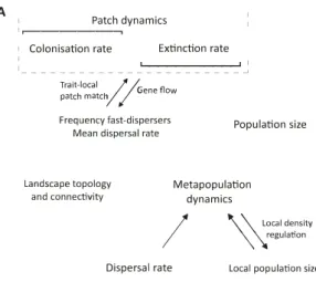
Spatial models allow for EEFs between local demography or metapopulation conditions and an evolving trait. The feedback can be modified by external properties such as patch dynamics ( colonization and extinction rates; Hanski & Mononen, 2011) or landscape structure (Kubisch et al., 2016; Fronhofer & Altermatt, 2017). In models with discrete habitat patches, dispersal is a central trait connecting local patches, and can have important effects on both ecological (Clobert et al., 2012) and evolutionary (e.g., can limit or favour local adaptation; Lenormand, 2002; Riisiinen & Hendry, 2008; Nosil et al., 2009) pro-cesses. The evolution of dispersal likely is the most frequently studied example of an EEF in fragmented landscapes (Legrand et al., 2017).

In a spatial model without dispersal evolution, Gomulkiewicz & Holt (1995) show that ER can be strongly hampered by stochasticity, for example, as a consequence of low population sizes (see Go-mulkiewicz et al., 1999, for another example of spatial ER). Interestingly, the probability of rescue can be a non-monotonie fonction of migration rates (Uecker et al., 2014). If dispersal is allowed to evolve (Ronce, 2007), it may be modelled as a discrete trait with dispersing and resident genotypes (e.g., Hanski & Mononen, 2011), as a quantitative trait (Hanski, 2011), or even as an evolving reaction norm (Travis & Dytham, 1999; Poethke & Hovestadt, 2002, for an overview on the genetics of dispersal and how disper­ sal is incorporated into models see Saastamoinen et al. 2018). For example, combining stochastic patch occupancy models with description of mean phenotypic changes in local populations, Hanski & Mononen (2011) studied an EEF between patch dynamics (colonisation and extinction) and the frequency of a disperser genotype ( for details see Fig. 3A).

A , Patch dynamics : '�----�

, Colonisation rate Extinction rate

:_

patch match// · ene ow Frequency fast-dispersers

Mean dispersal rate

Landscape topology and connectivîty Population size Meta population dynamics

I

Dispersal rate Local population size

Figure 3: Examples of studies with spatial feedbacks. (A) Study by Hanski (2011) and Hanski & Mononen (2011) where patch dynamics driven by colonisation and extinction might influence disperser frequency (Hanski & Mononen, 2011) or shifts mean dispersal rate (Hanski, 2011), which in turn influences patch dynamics. (B) Study by Fronhofer & Altermatt (2017) in which landscape topology influences dispersal evolution, which in turn influences colonization probabilities and metapopulation dynamics ( occupancy, turnover, genetic structure, global extinction risk).

In spatial models, EEFs can link processes at différent spatial scales. For instance, Poethke et al. (2011) show that the selective increase of patch size, e.g., as a conservation measure, can select against dispersal (eco-to-evo) which decreases re-colonization probabilities and can lead to ES (evo-to-eco). Evo-lution can also rescue populations from extinction which will depend on the rate of environmental change and landscape settings: ER may be found when environmental changes are not too fast (Schiffers et al., 2013), but the contrary has also been found (Boeye et al., 2013). Similarly, in a range expansion context, Burton et al. (2010) and Fronhofer & Altermatt (2015) showed that the ecological process of a range expansion can select for increased dispersal at range fronts (Travis & Dytham, 2002) and may feed back on the distribution of population densities across the range via life-history trade-offs. The importance of landscape structure for EEFs is laid out in Fronhofer & Altermatt (2017) (Fig. 3B). Taken together, spatial models may consider local adaptation to abiotic conditions as a heritable trait and fix dispersal or may consider dispersal as an evolving trait. Altogether, the studies show that dispersal is an excel­ lent candidate to link ecology (demography from a single population or metapopulation) and evolution, making dispersal central to EEFs.

4 EEFs involving two species

In multi-species systems, EEFs can be mediated by intra- and interspecific densities that affect fitness and trait distributions (Travis et al., 2013). In the following, we consider four major categories of two-species interactions: interspecific competition, predator-prey, parasite-hast and mutualistic interactions.

4.1 lnterspecific competition

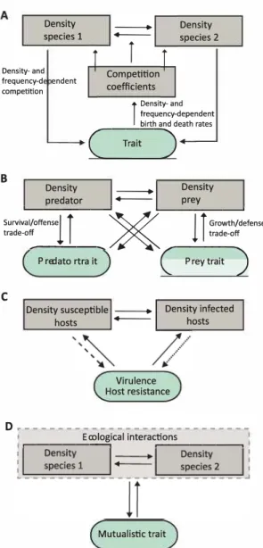
Interspecific competition is a reciprocal interaction for a shared limiting resource (Dhondt, 1989), such as food. In this interaction, the competing species can evolve different niches in order to coexist (Brown & Wilson, 1956; Abrams, 1986; Taper & Case, 1992). Many studies have shown that competition­ induced selection can result in adaptive divergence through ecological character displacement (Brown & Wilson, 1956; Slatkin, 1980; Taper & Case, 1992; Schluter, 2000). However, other studies have shown that competition could also lead to functional convergence of the competitors (Abrams, 1990; terHorst et al., 2010). In these models, EEFs may occur because competing species exert selection pressures that result in trait evolution (eco-to-evo) that might alter selection pressures on both species (evo-to-eco) (e.g., Vasseur et al., 2011, Fig. 4A). The earlier models of character displacement assume fixed variance and often Gaussian shapes for the species' character distribution (e.g., Slatkin, 1980). Recently, Sasaki & Dieckmann (2011) suggested the oligomorphic approximation as a way to describe the QG of an asexually reproducing population that consists of multiple morphs. Sasaki & Dieckmann (2011) then used this approach to gain a more detailed understanding on the dynamics of evolutionary branching in a resource competition model and showed among other aspects how to obtain threshold conditions for evolutionary branching and how mutations affect these conditions.

Models on interspecific competition include, for example, Dieckmann & Doebeli (1999). This study used an IBM, in which the evolving trait determines the carrying capacity (competition), and in which individuals survive and die via density- and frequency-dependence giving rise to a feedback between density and trait evolution, resulting in speciation via evolutionary branching. The authors showed that evolution of assortative mating can lead to reproductive isolation, resulting in increased diversity and that non-random mating is a prerequisite for evolutionary branching (see also Thibert-Plante & Hendry, 2009). In a similar model, Aguilée et al. (2013) found that landscape structure highly influences the outcome of diversity resulting from underlying dynamics of competition and assortative mating. The latter study used an IBM assuming density-dependent resource competition and stronger competition between individuals with similar trait values, inducing frequency-dependent selection and considered traits linked to resource utilization and to mate choice. Last, a model by terHorst et al. (2010) found that evolutionary convergence could occur in a multispecies model when less resources than species were present and when the intra- and interspecific competition coefficients were equal. In this model, the rate of competitive exclusion slows down as species become more similar to one another (evo-to-eco), giving species more time to evolve (eco-to-evo). In summary, prominent examples of EEFs in two-species competitive systems, focus on character displacement and potentially speciation. While analytical models using ODE and the AD framework are well established (see e.g., Kisdi, 1999), studies on two-species

interactions often make use of IBMs combined with GA to include a relatively high level of biological complexity. Density species 1

-

-î

Î

_____

--l __

î

�

l î

a -to- r -tr-a -it- c

.--P-re-y-tr-a -it-)

C

Density susceptible - Density infected

hasts - hasts

Virulence Host resistance

D

.---�----Ec_o_lo..;;,gical interac�ti _on_s ____ �

Mutualistic trait

Figure 4: Examples of studies in which feedbacks occur in two-species settings. (A) Study by Vasseur et al. (2011) in which the competition coefficients determining the strength of intra- and interspecific competition are modelled in fonction of an evolvable trait (growth or defence trait) under density- and frequency-dependent competition. (B) General figure on possible EEFs in predator-prey dynamics (de­ tailed in Cortez & Weitz, 2014). Generally, a trade-off between growth and predator defence is assumed in the prey population, and a trade-off between mortality and offence is assumed in the predator pop­ ulation. Density of the predator and prey can both influence trait evolution in the predator and prey population, which due to the previously described trade-off, determines predator and prey density. (C) General figure on possible feedbacks in host-parasite dynamics (see Luo & Koelle, 2013). In a model of virulence evolution, density of susceptible hosts determines the degree of virulence which feeds back to change the density of susceptible hosts (striped arrow). In a model on host resistance, density of the infected hosts determine the evolution of host resistance (dashed arrow), which in turn determines the density of both susceptible and infected hosts. (D) General representation of possible feedbacks in mutualistic interactions. Changes in the ecological interactions between species determine the evolution of a mutualistic trait, which, in tutn, can change the ecological interactions between species.

4.2 Predator-prey interactions

In a predator-prey interaction, one species acts as a predator feeding on the other species serving as prey. EEFs in predator-prey systems imply that predator densities may induce trait evolution, for example, in prey defence (eco-to-evo) resulting in consequent shifts in prey and predator densities (evo-to-eco; Fig. 4B). Many studies have found that rapid evolution in prey defence due to shifting predator abundances results in antiphase cycles rather than ¾-lag cycles predicted by non-evolutionary models (Yoshida et al., 2003, 2007; Becks et al., 2010). Additionally, feedbacks can stabilize or destabilize predator-prey dynamics depending on genetic variation and trade-off shapes (Abrams & Matsuda, 1997; Abrams, 2000; Cortez & Ellner, 2010; Cortez, 2016).

Predator-prey dynamics have been extensively studied using models of trait evolution of the prey (e.g. Abrams & Matsuda, 1997; Cortez, 2016; McPeek, 2017), the predator (Cortez & Ellner, 2010), or both (e.g. Cortez & Weitz, 2014; van Velzen & Gaedke, 2017, Fig. 4B). In all three instances EEFs were modelled using either separate equations for the ecological and evolutionary dynamics ( e.g. Abrams & Matsuda, 1997) or QG recursion equations or an approximation of those (van Velzen & Gaedke, 2017), using an AD approach (Marrow et al., 1996) or by using multiclonal LV equations (which are identical to 'ecological selection' models Jones & Ellner, 2007; Ellner & Becks, 2011; Yamamichi et al., 2011; Cortez & Weitz, 2014; Haafke et al., 2016). Including life-history trade-offs between defence and fecundity may lead to recurrent EEFs (Meyer et al., 2006; Huang et al., 2017).

Phenotypic plasticity has been found to play an important role in predator-prey EEFs and has been incorporated for example by Yamamichi et al. (2011), who found that plasticity in prey defence promotes stable population dynamics more than rapid evolutionary responses, although, plasticity was not advan­ tageous in stable environments. The evolution of plasticity has been studied by Fischer et al. (2014), who extended an LV model allowing for variation in plasticity among multiple genotypes of prey. The inclusion of such variation in models improved their ability to explain predator-prey dynamics. Overall, predator-prey EEFs are a classical example of feedbacks involving phase shifts and impacts on stability. These effects are classically modelled with ODEs. Recent work highlights the importance of incorporating both effects of genetic diversity and phenotypic plasticity to explain community dynamics (Yamamichi et al., 2011; Kovach-Orr & Fussmann, 2013).

4.3 Host-parasite interactions

In a host-parasite interaction, one of the species lives at the expense of the other species. Similar to predators, parasites can impose strong selection pressures on their hosts, for example resulting in the evolution of defences that can in turn impose selection on parasite traits. This process can lead to

complex co-evolutionary dynamics in spatial and non-spatial settings. Host-parasite interactions are often characterised by overlapping time scales between epidemiological and evolutionary processes owing to the rapid evolution of those systems. Yet, even when evolution is slower than the spread of disease, selection in host-parasite systems is characterised by strong density-dependent feedbacks, where changes in densities affect selection pressures on transmission, virulence and other parasite traits ( eco-to-evo), and the resulting trait changes in turn alter the ecological dynamics (evo-to-eco; Luo & Koelle, 2013, Fig. 4C).

The study of virulence evolution in parasites and pathogens is a key topic in the theoretical literature involving EEFs. The seminal work of Anderson & May (1982) showed that pathogen evolution is shaped by the epidemiological dynamics of infectious diseases through the density of susceptible hosts. Since then, a large literature has been devoted to understanding the effect of EEFs on the evolution of parasite virulence and host resistance (e.g. Lenski & May, 1994; Van Baalen, 1998; Boots & Haraguchi, 1999; Dieckmann et al., 2002; Frickel et al., 2016; Lion & Metz, 2018). Most models of host-parasite EEFs use classical epidemiological models ( compartment models that include susceptible, infected and potentially recovered individuals; SIR models) to describe the changes in density or frequency of susceptible and infected hosts. These epidemiological models are then coupled with AD (Dieckmann et al., 2002; Lion & Metz, 2018) or QG (e.g., Day & Proulx, 2004; Day & Gandon, 2007) approaches.

In the wake of Anderson & May (1982)'s seminal work, many studies have focused on the evolution of pathogen traits, under the assumption that host evolution is much slower and can be neglected. This has led to a good understanding of how EEFs affect pathogen evolution. A key insight is that, even if the host is assumed not to evolve, the time scales between ecology and evolution may either be decoupled (e.g., the pathogen evolves while the population is at an endemic equilibrium, see e.g. Dieckmann et al. (2002); Lion & Metz (2018) for a review of AD approaches) or overlap (e.g., when the pathogen evolves during an epidemic, see e.g.412004Day & Proulx,402007Day & Gandon for a QG formalism). What governs the difference

in time scales between epidemiology and pathogen evolution will then be the amount of standing genetic variation or the mutation rate.

More generally, coevolution between hosts and parasites with overlapping generation times has been studied (Nuismer et al., 2008; Eizaguirre et al., 2009; Best et al., 2010), in particular in the local adaptation literature (Nuismer et al., 2008), but often under the restrictive assumption of fixed demography, which sets strong limits to the types of EEFs that are possible. In contrast, other studies of coevolution have demonstrated how the dimension of the environment plays a critical role in governing evolutionary branching and diversification in both the host and the pathogen (Best et al., 2010). However, the study of EEFs in co-evolutionary host-parasite system remains underdeveloped. Interestingly, those systems appear to be particularly amenable to experiments and should allow researchers to further tease apart

the underlying effects of EEFs. For example, (Brunner et al., 2017) demonstrated that the sole presence of a fish parasite in an experimental ecosystem alters the abiotic environment of the host in terms of nutrient content or dissolved oxygen. These altered environments were shown to impose selection on a subsequent generation of hosts, hence evidencing that macroparasites can mediate eco-evolutionary feedbacks between fish and their environment.

Host-parasite interactions have also played a crucial role towards understanding spatial EEFs ( e.g., Boots & Sasaki, 1999; Boots et al., 2004, reviewed in Lion & Gandon 2015). These studies have often modelled space as a regular network of sites, in which each site is either empty or contains a single host individual, which can be either susceptible or infected. Such models can easily be analysed using IBMs, but analytical insight is also possible to some extent, using either AD or QG (Lion & Gandon, 2016). Due to the inherent complexity of spatial models, however, we only have a partial understanding of how the feedback between spatial epidemiological dynamics and the evolution of host and parasite traits unfolds in more realistic hast-parasite interactions (but see Nuismer et al., 2000, 2003). In summary, the host­ parasite literature has a long tradition of studying EEFs. Methodological approaches differ depending on the level of complexity, from simple ODEs to IBMs.

4.4 Mutualistic interactions

A mutualistic interaction implies that the interaction is beneficial for both partners involved (e.g., plant­ pollinator or host-symbiont interaction). EEFs in the context of mutualisms are expected to strongly impact the co-evolutionary process between mutualists and exploiters (eco-to-evo) which in turn shapes the ecological dynamics of the system (evo-to-eco; Fig. 4D; Doebeli & Knowlton 1998; Jones et al. 2009). EEFs were found to play an important role in determining phenotypic and population outcomes in an AD model on the coevolution of mutualists and exploiters when long-term coexistence of the species was possible (Jones et al., 2009). In the model by Jones et al. (2009), birth rates of the mutualist and exploiter were assumed to evolve and determine the nature of the mutualistic interaction. Ferrière et al. (2002) constructed a mathematical model combining simple Lotka-Volterra equations describing the ecological mutualistic interactions between the two species, with differential equations describing the evolutionary dynamics of the mutualistic traits. These evolutionary dynamics follow the fitness gradient shaped by the underlying ecological dynamics (eco-to-evo), which in turn determine the benefit of the mutualistic interaction ( evo-to-eco) [Fig. 4D].

Fewer studies have investigated the effect of spatial heterogeneity on mutualistic interactions, but those that have show that spatial heterogeneity can lead to long-term persistence of mutualism (e.g., Doebeli & Knowlton, 1998). Overall, mutualistic interactions in an eco-evolutionary context have been studied less compared to the other three interactions types discussed earlier. Nevertheless, studies have

shown that EEFs may play an important role for this type of interaction.

5 EEFs in a community and ecosystem context

The increasing interest in more complex ecological settings has resulted in a rapid growth of models focusing on communities and ecosystems that could simultaneously incorporate evolutionary dynamics (Brannstrom et al., 2012). Such models extend previous work to include niche construction, plant-soil feedbacks, multiple-species communities and foodwebs.

5.1 Feedbacks between organisms and abiotic environments

EEFs with the environment have been studied in the context of niche construction (Odling-Smee et al., 2003; Lehmann, 2008; Kylafis & Loreau, 2011), as in plant-soil feedbacks, for example (Schweitzer et al., 2014; Ware et al., this issue, Fig. 5A). Game theory has been used to investigate selection on niche constructing phenotypes (Lehmann, 2008) where the feedback arises when individuals affect their envi-ronment by reproducing (evo-to-eco), hence altering the selection pressure on the population (eco-to-evo). In plant-soil systems, plants might adaptively regulate soil fertility, resulting in positive, self-sustaining nutrient feedbacks that influence evolution. For example, increasing the direct benefit of soil nutrient conditioning to plants has been predicted to increase selection for higher values of soil conditioning traits (Kylafis & Loreau, 2008). Implicit in this model is a genetically based plant trait that links plants with their soils. Subsequent models have shown that these genetically based plant-soil links can re-sult in EEFs depending on the match with the soil gradient and the genetic variation present in the environment-altering plant trait (Schweitzer et al., 2014).

In plant-soil systems evolutionary change in plant traits can influence ecological dynamics of soil microbes (evo-to-eco) which in turn can change selection pressures on plant traits (eco-to-evo). This can be investigated using IBMs (Schweitzer et al., 2014) or by using an extended version of classical resource­ competition models (Eppinga et al., 2011). In this specific model, the decomposition of litter releases nutrients that can be taken up by the plants influencing competitive ability of the plant (eco-to-evo), resulting in different plant genotypes that might grow better. The change in the genetic composition of the plant population can in turn influence the litter pool (evo-to-eco).

In analogy to negative niche construction (Odling-Smee et al., 2003), the spatial structure of local negative feedbacks can result in changes in local diversity (e.g., Loeuille & Leibold, 2014). The environ­ ment becomes less suitable for the species occupying it (evo-to-eco), which induces a change in selection pressure on the species to evolve toward a more matching trait-environment value (eco-to-evo). Overall, plant-soil interactions are good examples of niche construction whereby EEFs can both be modelled and

B

C

Environment (abiotic) Soil (community) property

�production Niche constructing trait

Plant trait Community

diversity

Physical loca� \ Reprod�c_tion in space _{\ �mpetitio}n

Trait species i

Food web structure Species interactions

l î

î

Figure 5: Examples of studies in which feedbacks occur between abiotic and biotic component or in a multi-species settings. (A) General figure of EEFs in niche construction (Lehmann, 2008; Kylafis & Loreau, 2011) and plant-soil feedbacks (Schweitzer et al., 2014). In niche construction the abiotic environment determines the evolution of a trait that modifies this abiotic environment. Similarly, in a plant-soil system, a plant trait can modify the soil, which drives evolution of plant traits. (B) Study by Martin et al. (2016) in which trait values and spatial locations species determine competition, changing local selection pressures, resulting in shifting local and global trait distributions and community diversity. (c) Study by Ito & Ikegami (2006), in which each species has a separate prey and predator strategy which results in clusters of trophic species arising from changing interactions between species, which in turn continuously change the position, shape and size of occupied areas in phenotypic space and change trophic interactions resulting in further phenotypic evolution and eventually evolutionary branching and the emergence of foodweb structure.

observed in nature. The methods employed range from formal mathematical approaches to IBMs.

5.2 Feedbacks within communities

Theoretical studies on EEFs in multi-species communities can increase our understanding of biodiversity (Patel et al., 2018). Eco-evolutionary analyses have led to new insights into coexistence theory, the maintenance of diversity, as well as the structure and stability of communities (Kremer & Klausmeier, 2017; Patel et al., 2018). Moreover, studies have found that evolution might maintain (Martin et al., 2016), increase (e.g. via speciation or ER Rosenzweig, 1978; Dieckmann & Doebeli, 1999; Gomulkiewicz & Holt, 1995) or decrease (Norberg et al., 2012; Kremer & Klausmeier, 2013; Gyllenberg et al., 2002)

phenotypic, species and functional diversity.

For example, Martin et al. (2016) show that EEFs can maintain phenotypic diversity. The authors combine niche based approaches with neutral theory in a spatially structured IBM where each individ­ ual has a location in space and is constrained by a specific trade-off between resource exploitation and competition. Similar individuals experience higher competition resulting in frequency-dependent selec­ tion. Competition only takes place between neighbouring individuals, changing local selection pressures, which results in local evolutionary shifts in phenotypic traits (eco-to-evo) that shift the global pheno­ typic trait distribution and influence species differentiation and thus community diversity (evo-to-eco; Fig. 5B). By contrast, Norberg et al. (2012) found that the eco-evolutionary processes induced by cli­ mate change continued to generate species extinctions long after the climate had stabilized, and thus resulted in further diversity loss. These authors used a spatially explicit eco-evolutionary model based on partial differential equations to predict species responses to climate change in a multi-species context in which they allowed genetic variation and dispersal to jointly influence ecological ( competition and species sorting) and evolutionary (adaptation) processes. The findings of both studies discussed above can eas-ily be understood in the light of modern coexistence theory (reviewed in Chesson, 2000) as they relate to stabilizing ( concentrating intraspecific interaction by dispersal limitation) and equalising mechanisms (sorting). In summary, EEFs in communities emerge, because species' traits may affect the community and, vice versa, the community context may affect trait evolution (terHorst et al., 2018). Interestingly, fitness may not only depend on densities, but also on total community biomass, total productivity, or even on species richness. Consequences of evolutionary change can be understood in the light of modern coexistence theory.

5.3 Feedbacks in food webs

Evolutionary dynamics have been suggested to determine food web structure (Rossberg et al., 2006). Hence, there has been an upsurge in studies including evolutionary dynamics into food web models, by allowing a recurrent addition of new species or morphs into the food web, based on the theory of self­ organized criticality (Bak et al., 1987; Caldarelli et al., 1998; Drossel et al., 2001; Rossberg et al., 2006; Allhoff & Drossel, 2013; Bolchoun et al., 2017). These evolutionary food web models often depend on a trait that shapes the biotic interactions which determine the food web structure. Food web structure selects the species that remain in the system (eco-to-evo), which in turn alters the phenotypic trait distribution in the system on which mutations can occur to create a new species or morphs. The addition of a new species or morph changes the present species interactions (evo-to-eco), hence changing the food web structure (Bolchoun et al., 2017). This interplay between population dynamics and morph evolution determines the EEF, and shapes the structure of the food web. Similar to the AD framework, it is

assumed that ecological dynamics occur fast and reach ( quasi)equilibrium, while evolutionary dynamics occur on a much slower time scale (Guill & Drossel, 2008; Allhoff & Drossel, 2013). Studies including both ecological and evolutionary processes in food web models show that this can lead to new insights in food web dynamics as opposed to models that only include fixed ecological dynamics (Bolchoun et al., 2017).

Most studies on food web models focus on speciation-extinction dynamics with species being the unit of the model, while fewer studies have investigated how the evolution of traits results in food web formation (Ito & Ikegami, 2006; Takahashi et al., 2013). Both Ito & Ikegami (2006) and Takahashi et al. (2013) have modelled the built up of a food web through evolutionary dynamics by attributing to each individual or phenotype a prey and predator trait (resource or vulnerability, respectively, utilization or foraging). Individuals are assumed to reproduce asexually and offspring may differs lightly because of small random mutations. Ito & Ikegami (2006) show that isolated phenotypic clusters of species and the emergence of higher trophic levels arise due to changing interactions between species (eco-to-evo), which in turn continuously changes the position, shape and size of occupied areas in phenotypic space. These changes, in turn, alter trophic interactions (evo-to-eco) resulting in further phenotypic evolution and eventually evolutionary branching (Fig. 5C). Takahashi et al. (2013) used an IBM to show that initial phenotypic divergence in the foraging trait relaxes interference competition (eco-to-evo), which results in the emergence of species clusters. The resulting changes in species interactions (trophic levels; evo-to-eco) mediate further divergence in foraging traits and predator vulnerability (eco-to-evo). A study by de Andreazzi et al. (2018) explicitly evaluated the effects of network structure on eco-evolutionary dynamics for long-term ecological network stability, by using different antagonistic species networks in their simulations. Population dynamics were modelled to depend on the phenotypic trait, while mean trait evolution depended on the environment and the antagonistic species interactions. The authors showed that EEFs resulted in specific patterns of specialization which led to increases in species mean abundances and to decreases in temporal variation in abundances.

The effects of spatial dynamics on food web structure has also been studied. For example, (Loeuille & Leibold, 2008), combined a simple food web structure (specialist and generalist herbivore species feeding on two plants which in turn feed on nutrient resources), with a 12-patch metacommunity to evaluate the interactions between evolutionary adaptation and community assembly dynamics as a fonction of dispersal. The two plant species had quantitative and qualitative defence traits that were heritable, upon occurrence of small mutations between each time steps. The authors found that the occurrence of dispersal between patches led to the evolution of distinct morphs of the plant species (eco-to-evo), which influenced the trophic and food web structure in local patches (evo-to-eco).

analysis of these feedbacks remains rare. This is probably due to the main assumption of the separation of time scales of ecology and evolution, with mutation being considered equivalent to speciation Takahashi et al. (2013), and traits remaining constant within species. Exceptions exist of course, such as the food web model used by Loeuille & Leibold (2008). However, especially meta-foodweb models are scarce

(Urban et al., 2008) Evolutionary food web models have promising features that may result in a better

understanding of EEFs in more complex (natural) scenarios and likely represent one of the current major

challenges in eco-evolutionary modelling (Melian et al., 2018).

6 Synthesis and conclusions

Throughout this overview, we found that EEFs have been incorporated into theoretical models across a wide range of different levels of biological organization. The relevance of the EEF may not only depend on the biological system, but also on the specific traits used: different effects may be found depending on whether the trait is influenced by the ecological property or not (e.g., densitydependent versus -independent traits). Not surprisingly, including EEFs in theoretical models significantly changes our view of well-known patterns emerging from pure ecological or pure evolutionary models ( e.g., Dieckmann

& Metz, 2006; Poethke et al., 2011). More specifically, we have identified models that include EEFs, whose

underlying formalisms fall into a few categories (Fig. lB). In principle, any modelling framework that couples ecological dynamics (e.g., ODEs, IBMs) with an evolutionary model (e.g., QG, AD or GA) can be useful for studying feedbacks. Studies modelling intertwined ecological and evolutionary dynamics most often differ in their assumption of the time scale at which ecological and evolutionary processes occur. Studies assuming contemporary ecological and evolutionary dynamics often couple ODEs with QG or use IBMs, while studies assuming evolution to occur when ecological dynamics are at equilibrium couple demographic models with AD ro make analogous assumptions.

6.1 Conclusions to date

Based on our non-exhaustive overview of theoretical work on EEFs, a few general conclusions emerge: First, EEF models explicitly include ecological dynamics in the analyses of evolutionary processes, and vice versa. Density- and frequency-dependent selection are often key ingredients for EEFs. In many cases, density- and frequency-dependency, as well as ecological stochasticity are not a priori assumptions, but emerge from ecological settings and trait correlations, for example. Second, EEFs are not new to evolutionary ecology theory - they are deeply rooted in the theory of many subdisciplines. For instance, the predator-prey and host-parasite literature, speciation literature and evolutionary branching, character displacement, as well as metapopulation modelling or niche construction theory naturally incorporate

EEFs. Strikingly, while the field of (meta)community ecology is rather new (Leibold et al., 2004), EEFs seem to have been included in (meta)community ecology very rapidly, culminating in the recognition that the basic drivers of evolution and community ecology are analogous (Vellend, 2010). Third, in a spatial setting dispersal is a primary candidate for successful eco-evolutionary linkages, because dispersal is both an ecological process impacting densities and, at the same time, mediates evolution via gene flow. In addition, it is itself subject to evolution (Ronce, 2007). Movement can be similarly important (Hillaert et al., 2018). Fourth, EEFs do not necessarily require rapid or contemporary evolution (Post & Palkovacs, 2009). Of course, contemporary evolution has sparked a lot of interest in EEFs (Hendry, 2017), but feedbacks are also possible over longer timescales ( e.g., as shown in AD models). Fifth, our short overview of the eco-evolutionary modelling toolbox clearly highlights that the main character of an eco-evolutionary model is the combination of demographic and evolutionary models, regardless of the concrete formalism.

Because different formalisms originate from different fields, they often rely on differing assumptions. For instance, the time scales on which processes occur and the sources of genetic variation are important consideration of the different modelling formalisms (Lande, 2007; Srether & Engen, 2015). This has made some formalisms more focussed on analysing evolutionary end-points and long-term dynamics (AD), while others have focused on short-term dynamics from one generation to the next (QG). However, in both formalisms incorporating EEFs is feasible. The separation of time scales also means that the form of the feedback may change when we move from one dynamical regime to the other, which has been well studied in host-parasite models (Lenski & May, 1994; Day & Gandon, 2007; Gandon & Day, 2009; Lion, 2018). However, most interest probably lies in predicting the mid-term dynamics of an EEF system. To approach this properly, an important issue for future theoretical work will be to develop mechanistic models for the dynamics of phenotypic and genotypic variation in populations evolving at this mid-term time scale of tens to hundreds of generations (see Fig. 6 for an individual-based perspective). This would reveal for instance whether EEFs are time dependent and how common they are expected to be. However, to couple these models to natural systems, one needs to measure heritability and genetic ( co )variances of traits which can be challenging.

Our review also underlines the pervasive nature of EEFs. It seems at best difficult to design a model that includes ecology and evolution without an EEF (see also Hendry, 2017, chapter 1 for a discussion). However, it is possible that some traits have little effect on the ecological dynamics, or that some ecological variables will have little effect on the evolutionary dynamics. For instance, in a discrete-time model, if absolute fitness is proportional to a fonction of density, say Wi(t)

=

evolutionary dynamics: the focal trait average steadily increases and resource density decreases until a maximum (resp. minimum) is reached. Such simplistic EEFs have been termed frequency-independence in the broad sense by Metz & Geritz (2016). Overall, recent models have become more elaborate. However, increased complexity and realism often trades off with tractability. As a consequence these studies must provide additional tests that either involve models where the presumed feedback is absent, or provide a simplified analytical model (e.g., Kubisch et al., 2016; Branco et al., 2018, for examples involving IBMs).

6.2 The way forward

The challenge today consists in pursuing new, more integrative and mechanistic modelling avenues which have the potential to include different aspects of realism, such as genotype-phenotype mapping, plasticity as well as population and spatial structure (Fig. 6) and predicts of mid-term dynamics of EEFs as outlined above. Current theory has greatly increased our understanding of EEFs (McPeek, 2017), but these feedbacks have been primarily explored within hierarchical levels of ecosystem organization, be they spatial or temporal hierarchies, and have often involved only single or a few independently evolving traits. While the presence of a hierarchical organization of ecosystems is well established (Melian et al., 2018), it is an ongoing challenge to identify the relevant hierarchical levels and their interdependencies to understand EEFs.

Currently, the leading graphical model adopts an implicit hierarchy with feedbacks between levels from genes, to traits, to populations, to communities, to ecosystem processes (Hendry, 2017, see also Fig. lA for a simplification). Making such a conceptual model more mechanistic requires understanding how interactions at one scale (gene regulatory networks or complex traits) affect processes at different scales (trait-dependent species interactions). One such modelling attempt by Melian et al. (2018) links ecological and evolutionary networks in a meta-ecosystem model, taking into account demography, trait evolution, gene flow, and the ecological dynamics of natural selection. Such process-based models can yield new insights into the mechanistic basis of EEFs in more complex natural scenarios. Sorne of the most important processes are summarized in Fig. 6 which expands the conceptual model presented in Fig. lA to a more mechanistic level. With this representation we propose that feedbacks are best conceptualized as emerging from individual-level interactions (see also Rueffier et al., 2006), with dispersal and interactions with the abiotic environment leading to the emergence of the relevant hierarchical complexity.

Besides theoretical advances, connecting theory to controlled laboratory or field experiments more tightly will allow for the experimental assessment of theoretical predictions about feedbacks. For exam-ple, using rotifer-algae chemostats Yoshida et al. (2003) experimentally tested predictions of a theoretical predator-prey model that allowed for prey evolution. This experiment confirmed the anti-phase oscil-lations predicted from theory when prey evolves defence strategies. While such prominent examples of

biotic interactions birth, death, dispersal individual i abiotic environ ment selection, drift, gene flow phenotype ' plasticity ' _\ \ \ 1 ,' genetic change and map to phenotype mutation

Figure 6: Mechanistic underpinnings of EEFs. Ecological dynamics (left) are driven by individual-level properties (birth, death, dispersal). Interactions between individuals of the same or different species (biotic interactions) impact these properties, which may lead to density-dependence, for example. Indi­ viduals internet with the abiotic environment and vice versa. Importantly, these ecological settings will impact selection, drift and migration (eco-to-evo). Evolution is governed by the interaction between these processes, genetic constraints and mutations. The resulting phenotype is subsequently determined by the genotype-phenotype map. Ultimately, the phenotype will impact ecology (evo-to-eco) by changing births, death, dispersal and the abiotic environment. Plasticity (dashed lines) may modulate the phenotype and, hence, the dual effects of the organism on biotic and abiotic environments.

the integration of theory and empirical data on EEFs exist (see among others also, Metcalf et al., 2008; Litchman et al., 2009; Becks et al., 2012; Thomas et al., 2012; Fischer et al., 2014; Fronhofer & Altermatt, 2015; Huang et al., 2017; Bonte & Bafort, this special issue; De Meester et al., this issue; Van Nuland et al., this issue) given the breadth of the theoretical work highlighted here, the coupling of empirical data from natural and experimental settings, with theoretical models needs to be deepened. This gap between theory and empirical work may, in part, be due to differences in technical jargon that impede effective communication between theoreticians and empiricists as well as modelling specializations among theoreticians which impede synthesis or at least slow down progress. Isolation among subdisciplines and methods leads to confusion, reduced inference and will not advance the field. In the latter case, efforts such as those of Queller (2017) and Lion (2018) at unifying theoretical fields are urgently needed. To advance theory on EEFs, we here suggest that taking a mechanistic approach focused on individual-level traits (Rueffier et al., 2006) as outlined in Fig. 6 can be productive for developing novel and synthetic theory. Key ingredients to such an individual-level approach is the description of focal organisms in terms of individual properties (age, ecologically important traits, life history parameters), and linking these to demographic processes (see also Travis et al., 2014). Most importantly, scientists need to learn to appre-ciate the strengths of their respective approaches, be they theoretical, experimental laboratory-based or comparative, and not focus on the weaknesses to discard possible avenues of collaboration and progress. Clearly, bridging between theory and empirical data is more difficult when studying ecology and evolu-tion in the wild (Hendry, this issue) and ecological pleiotropy may even cancel out EEFs (DeLong, 2017).