HAL Id: hal-00317653
https://hal.archives-ouvertes.fr/hal-00317653
Submitted on 30 Mar 2005
HAL is a multi-disciplinary open access
archive for the deposit and dissemination of
sci-entific research documents, whether they are
pub-lished or not. The documents may come from
teaching and research institutions in France or
abroad, or from public or private research centers.
L’archive ouverte pluridisciplinaire HAL, est
destinée au dépôt et à la diffusion de documents
scientifiques de niveau recherche, publiés ou non,
émanant des établissements d’enseignement et de
recherche français ou étrangers, des laboratoires
publics ou privés.
The association of coronal mass ejections with their
effects near the Earth
R. Schwenn, A. Dal Lago, E. Huttunen, W. D. Gonzalez
To cite this version:
R. Schwenn, A. Dal Lago, E. Huttunen, W. D. Gonzalez. The association of coronal mass ejections
with their effects near the Earth. Annales Geophysicae, European Geosciences Union, 2005, 23 (3),
pp.1033-1059. �hal-00317653�
SRef-ID: 1432-0576/ag/2005-23-1033 © European Geosciences Union 2005
Annales
Geophysicae
The association of coronal mass ejections with their effects near the
Earth
R. Schwenn1, A. Dal Lago2, E. Huttunen3, and W. D. Gonzalez2
1Max-Planck-Institut f¨ur Sonnenystemforschung, D 37191 Katlenburg-Lindau, Germany 2Instituto Nacional de Pesquisas Espaciais, Sao Jose dos Campos, SP, Brazil
3Department of Physical Sciences, P.O. Box 64, FIN-00014, University of Helsinki, Finland
Received: 19 August 2004 – Revised: 19 November 2004 – Accepted: 13 January 2005 – Published: 30 March 2005
Abstract. To this day, the prediction of space weather
ef-fects near the Earth suffers from a fundamental problem: The radial propagation speed of “halo” CMEs (i.e. CMEs pointed along the Sun-Earth-line that are known to be the main drivers of space weather disturbances) towards the Earth cannot be measured directly because of the unfavor-able geometry. From inspecting many limb CMEs observed by the LASCO coronagraphs on SOHO we found that there is usually a good correlation between the radial speed and the lateral expansion speed Vexp of CME clouds. This
lat-ter quantity can also be delat-termined for earthward-pointed halo CMEs. Thus, Vexp may serve as a proxy for the
oth-erwise inaccessible radial speed of halo CMEs. We studied this connection using data from both ends: solar data and in-terplanetary data obtained near the Earth, for a period from January 1997 to 15 April 2001. The data were primarily pro-vided by the LASCO coronagraphs, plus additional informa-tion from the EIT instrument on SOHO. Solar wind data from the plasma instruments on the SOHO, ACE and Wind space-craft were used to identify the arrivals of ICME signatures. Here, we use “ICME” as a generic term for all CME effects in interplanetary space, thus comprising not only ejecta them-selves but also shocks as well. Among 181 front side or limb full or partial halo CMEs recorded by LASCO, on the one hand, and 187 ICME events registered near the Earth, on the other hand, we found 91 cases where CMEs were uniquely associated with ICME signatures in front of the Earth. Eighty ICMEs were associated with a shock, and for 75 of them both the halo expansion speed Vexpand the travel time Tt rof the
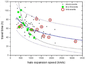
shock could be determined. The function Tt r=203–20.77* ln
(Vexp)fits the data best. This empirical formula can be used
for predicting further ICME arrivals, with a 95% error mar-gin of about one day. Note, though, that in 15% of com-parable cases, a full or partial halo CME does not cause any ICME signature at Earth at all; every fourth partial halo CME and every sixth limb halo CME does not hit the Earth (false
Correspondence to: R. Schwenn
(schwenn@linmpi.mpg.de)
alarms). Furthermore, every fifth transient shock or ICME or isolated geomagnetic storm is not caused by an identifiable partial or full halo CME on the front side (missing alarms).
Keywords. Interplanetary physics (interplanetary shocks) –
Magnetospheric physics (Storms and substorms) – Solar physics, astrophysics and astronomy (flares and mass ejec-tions)
1 Introduction
Our modern hi-tech society has become increasingly vul-nerable to disturbances from outside our Earth system, in particular to those initiated by explosive events on the Sun. The economic consequences are enormous (see, e.g. Siscoe, 2000). That’s one reason why space weather and its pre-dictability have recently attained major attention, not only with the involved scientists but also with the general public. Another reason is the new quality of observational data that have been obtained over the last decade from a new gener-ation of space-based instruments. They have allowed ma-jor advances, among others, in the understanding of the pro-cesses involved near the Sun, in interplanetary space, and in the near-Earth environment (see, e.g. the review by Crooker, 2000).
Unfortunately, the preciseness of predictions of space weather effects is still poor. Solar energetic transients, i.e. flares and coronal mass ejections (CMEs), occur rather spon-taneously, and we have not yet identified unique signatures that would indicate an imminent explosion and its probable onset time, location, and strength. The underlying physics is not yet sufficiently well understood. Solar energetic par-ticles, accelerated to near-relativistic energies during major solar storms arrive at the Earth’s orbit within minutes (see, e.g. Garcia, 2004) and may, among other things, severely en-danger astronauts on the way to the Moon or Mars. But we have no appropriate warning tool yet!
1034 R. Schwenn et al.: The association of coronal mass ejections
1
Figure 1. The X17 flare and the halo CME of 28 October 28, 2003, as seen by the SOHO
instruments EIT (a), LASCO C2 (b) and C3 (c). This most dramatic event caused major
disturbances of space weather and affected the Earth system in various ways: charged particles
were accelerated to near-relativistic energies, such that they could penetrate spacecraft skins and
disturbed, e.g., the CCD cameras on SOHO (see c) and other satellite instrumentation, an
extremely fast interplanetary shock wave was initiated that reached the Earth only 19 hours later,
a severe geomagnetic storm (Dst –363 nT) was launched, with bright aurora even all over Europe
and the US. That was about 7 hours later than predicted using the tool described in this paper.
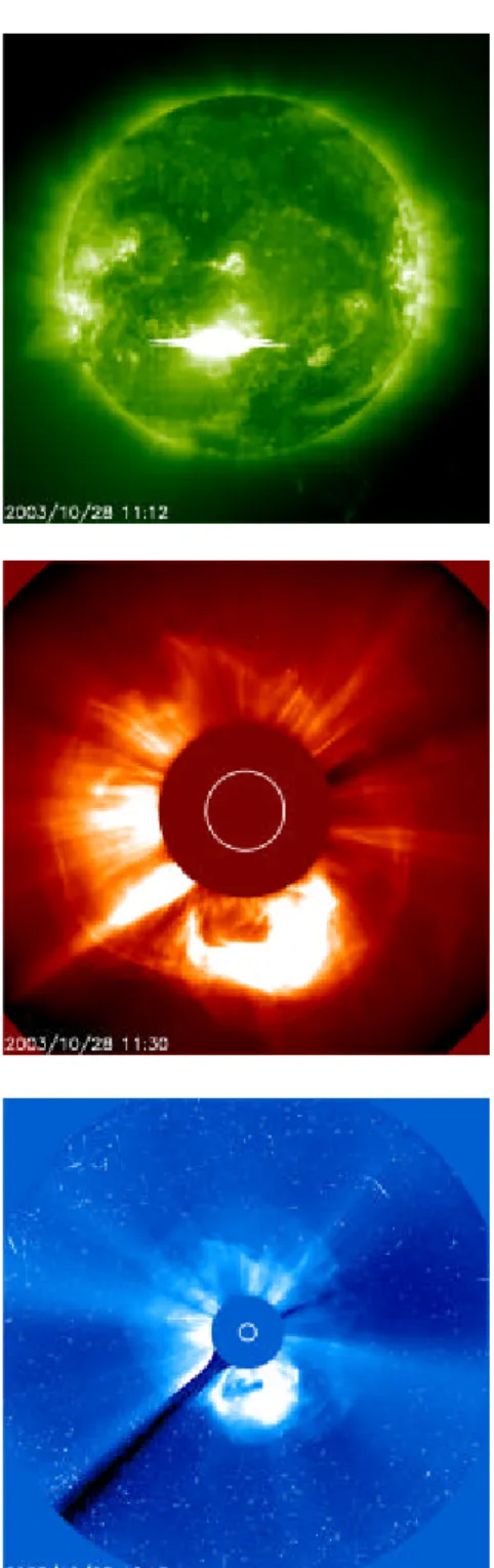
Fig. 1. The X17 flare and the halo CME of 28 October 2003, as
seen by the SOHO instruments EIT (a), LASCO C2 (b) and C3
(c). This most dramatic event caused major disturbances in space
weather and affected the Earth’s system in various ways: charged particles were accelerated to near-relativistic energies, such that they could penetrate spacecraft skins and disturbed, for example, the CCD cameras on SOHO (see c) and other satellite instrumenta-tion; an extremely fast interplanetary shock wave was initiated that reached the Earth only 19 h later; a severe geomagnetic storm (Dst
−363 nT) was launched, with bright aurora even all over Europe and the US. This was about 5 h earlier than predicted using the tool described in this paper.
Even once a notable outbreak has actually been observed, it is still hard to predict whether the ejected gas clouds will reach the Earth at all, at which time and what their effects will be. (The interplanetary counterparts of CMEs are often called “ICMEs”. In this paper, we use this term in a more generic way, such that it comprises all CME effects in inter-planetary space, i.e. not only the ejecta themselves but tran-sient shocks as well.) This is the main aspect to be addressed in this paper.
Of crucial importance is to determine the direction in which an eruption is originally pointed, since only one out of ten CME events hits the Earth (see, e.g. Webb and Howard, 1994 and St. Cyr et al., 2000). Space-based coronagraphs keep providing spectacular views of erupting gas clouds (see, e.g. the Web page http://star.mpae.gwdg.de/release/movieg. html) but they show just their projections onto the plane of the sky and do not allow to infer the ejection direction. CMEs pointed along the Earth-Sun line appear as “halos” around the occultor disk in a coronagraph’s field-of-view (Howard et al., 1982). Complementary disk observations are required for deciding whether a halo CME is pointed towards or away from the Earth. The value of such con-certed observations has been demonstrated ever since the set of modern solar telescopes on the Solar and Heliospheric Observatory (SOHO) spacecraft went into operation in early 1996 (Plunkett et al., 1998; Thompson et al., 1998). The disk images taken by the EUV Imaging Telescope (EIT, De-laboudini`ere et al., 1995; Delann´ee et al., 2000) at a suf-ficiently high time cadence allow almost continuous detec-tion of flare explosions and filament erupdetec-tions. Simultane-ously, the instruments C1 (no longer operating since June 1998), C2, and C3 of the Large Angle and Spectrometric Coronagraph (LASCO, Brueckner et al., 1995) observe the corona above the solar limb in a range from 1.1 Rs from
Sun center out to 32 Rs, with unprecedented sensitivity. In
Fig. 1 we show a typical example of a halo CME as ob-served by EIT, C2 and C3. Such images and animated se-quences plus data from other instruments both in space and on the ground are available on the Internet almost in real time (see, e.g. http://sohowww.estec.esa.nl). Many professional and amateur space weather analysts are routinely taking ad-vantage of their sites (e.g. http://www.sec.noaa.gov/today. html, http://sidc.oma.be, http://www.estec.esa.nl/wmwww/ wma/spweather/, http://www.spaceweather.com/, http://dxlc. com/solar/).
Of particular value are the messages the LASCO opera-tions team issues for any halo CME as soon as it appears (http://lasco-www.nrl.navy.mil/halocme.html). Some char-acteristic data, such as exact timing, angular span, front speed (also called “plane of the sky speed”) and position angle of the fastest feature, any potential association with flares and other events seen by EIT, are also given, and images and movies are made accessible through the In-ternet: ftp://ares.nrl.navy.mil/pub/lasco/halo. Detailed in-formation on all CMEs, including halos, is listed under http://cdaw.gsfc.nasa.gov/CME list/.
The mere knowledge of a halo’s general direction means an enormous step forward. The “away” events that are usu-ally not geo-efficient can now be revealed right away. How-ever, for the “toward” events the arrival times at Earth remain hard to predict, since the line-of-sight speed of a halo CME cannot be measured directly.
The data catalogs show that the CME front speeds vary widely between 200 km/s and more than 2000 km/s, i.e. by a factor of 10. However, for those cases with a uniquely rec-ognizable arrival of ICME effects at Earth, the travel speeds vary by not more than a factor of 3 (see, e.g. Cane et al., 2000; Gopalswamy et al., 2000). Apparently, the faster ICMEs are significantly decelerated (Woo et al., 1985, see also, e.g. Watari and Detman, 1998, and references therein), and the slower ones are post-accelerated in the ambient solar wind flow (Lindsay et al., 1999b). Brueckner et al. (1998), based on a number of 8 cases then known, had even concluded that the travel time of most ICMEs from the Sun to the Earth (measured from the first appearance in C2 images to the be-ginning of the maximum Kpindex of an associated
geomag-netic storm) always amounts to about 80 h, regardless of the halos’ behavior close to the Sun. Brueckner’s “80 h rule”, as the most simple prediction tool, appears to work pretty well in many cases, in particular near activity minimum. Sev-eral researchers have tried to find relationships between CME properties and ICME signatures, “with an eye towards space weather forecasting”, as Lindsay et al. (1999b) phrased it. Gopalswamy et al. (2000) determined from coronagraph im-ages the speed of the fastest moving halo CME feature, i.e. its speed VP S projected on the plane of the sky, and
com-pared it with the transit time of the associated ICME towards 1 AU, as defined by the in-situ appearance of intrinsic ICME signatures, i.e. magnetic clouds and low plasma beta. It is here where Gopalswamy et al. (2000) differ from other au-thors who used the onset of associated geomagnetic effects (e.g. Brueckner et al., 1998; Wang et al., 2002a). Assum-ing a global, effective acceleration/deceleration representAssum-ing the solar wind ICME interaction, Gopalswamy et al. (2000) derived a simple relation between the initial speed VP S of
a CME and its propagation. The authors consider this a first step towards a future predictive tool, although the travel times derived using their scheme deviate considerably from the observed travel times. Further studies (e.g. Webb et al., 2000; Cane et al., 2000; Gopalswamy et al., 2001c; Vrˇsnak and Gopalswamy, 2002; Michalek et al., 2002; Gonz´alez-Esparza et al., 2003a,b; Yurchyshyn et al., 2003) tried to improve the prediction accuracy, but they all keep suffering from the problem of deducing the proper propagation speed of ICMEs. In a recent analysis Burkepile et al. (2004) stud-ied that projection effect by selecting a subgroup of 111 limb CMEs observed by the Solar Maximum Mission (SMM). Not only do these limb CMEs have, on average, greater speeds than the average values obtained from all SMM CMEs (see Hundhausen, 1993), they also come from lower latitudes and have smaller cone angles. All this provides strong evidence that projection effects systematically influence the apparent CME properties.
2
Figure 2. The halo CME of 5 November 1998 (E90), for illustration of the different meaning of
expansion speed V
expand the plane of the sky speed V
P S. In this case we measured V
exp= 1116
km/s, and V
P S= 1118 km/s, A shock arrived at the Earth 55.6 hours later, i.e., about 7 hours
earlier than we predicted (case E20 in Table 2). A severe magnetic storm (D
st–142 nT) peaked
14 hours after shock arrival. The images are running differences between LASCO C3 images.
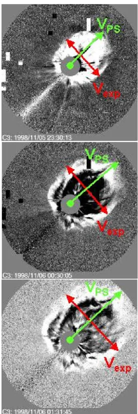
Fig. 2. The halo CME of 5 November 1998 (E90), for illustrationof the different meaning of expansion speed Vexpand the plane of
the sky speed VP S . In this case we measured Vexp=1116 km/s,
and VP S=1118 km/s, A shock arrived at the Earth 55.6 h later, i.e.
about 7 h earlier than we predicted (case E20 in Table 2). A severe magnetic storm (Dst −142 nT) peaked 14 h after shock arrival. The
1036 R. Schwenn et al.: The association of coronal mass ejections
Figure 2 illustrates the problem: The plane of the sky speed VP S as defined in the figure is containing almost
in-evitably a component resulting from a projection effect. In the case of the 11 November 1998 halo CMEs, the ejection is apparently pointed to the northwest. This is consistent with the location of the associated M8 flare at N18 W21. Needless to say, an observer located somewhere else in the heliosphere would have determined a different value of VP Sfor the same
CME, in contrast to Vexp, the speed of lateral expansion.
The work by Plunkett et al. (1998) made use of the ob-servation that the outer boundaries of most limb CMEs form a cone of constant spread with a median angular extent of
about 50◦. This was confirmed for many more limb CMEs
by St.Cyr et al. (2000). Adopting this value and knowing the projection speed VP S of a halo’s outer rim they inferred
a value around 600 km/s for its true frontal speed. Based on similar considerations, Zhao et al. (2002) derived their “cone model” of halo CMEs. They tried to fit 3 free parame-ters (angular width, latitude and longitude of cone axis) such that an observational image sequence is met best. This way, they inferred geometric and kinematic properties for the 12 May 1997 CME. However, they had to admit that “there are limitations for some halo CMEs”. Michalek et al. (2003), also using a cone model, derived the cones’ parameters by taking into account the moments of first appearance of the CME above opposite limbs on the occultor edge. No con-clusive results were obtained, though, which is due – in the authors’ opinion - to several shortcomings, for example, pos-sible acceleration and expansion of CMEs, missing symme-try of CMEs.
In some cases, interplanetary shocks on their way through the heliosphere generate type II radio emission at the local plasma frequency and its harmonics. This provides a means of remotely observing and even tracking ICMEs (LeBlanc et al., 2001, see also Reiner et al., 1998 2003b and ref-erences therein). This technique has been used for study-ing ICME dynamics and interactions (Reiner et al., 2003b; Gopalswamy et al., 2001a,b, 2002a,b; Lara et al., 2003), but usually after the fact. For near-real-time predictions the type II radio emission is only of limited value.
The basic task remains to find and measure early on the op-timum proxy data for the otherwise inaccessible propagation speed of a halo CME towards an observer. In analogy, one would have to measure the speed of a car approaching head-on. This is usually achieved by RADAR techniques, but nothing similar works out in the case of head-on CMEs. Al-ternately, one could measure how fast the car’s image grows in a telescope’s field-of-view. The apparent lateral expan-sion speed is a unique measure of the unknown line-of-sight speed. In fact, Fred Hoyle (1957) in his book “The Black Cloud” let a clever scientist calculate the arrival time of a deadly cloud approaching the Earth from deep space using the apparent expansion alone. Upon this warning, mankind was able in time to take provisions for survival. Based on this idea, we developed a similar, purely empirical technique. It makes use of the following well-established observational facts:
1. The cone angles of CME expansion and, more gener-ally, the shapes of the expanding CMEs are usually well maintained (Plunkett et al., 1998). The CME shapes remain “self-similar”. We remember that Low (1982) had already noticed the “often observed coherence of the large-scale structure of the moving transient”, which could be explained by what he called “self-similar evo-lution”. He studied the expulsion of a CME quantita-tively on the basis of an ideal, polytropic, hydromag-netic description and found self-similar solutions that describe the main flows of white-light CMEs as they are observed (see also Low, 1984; Gibson and Low, 1998; and Low, 2001).
2. We found it surprising in our inspection of hundreds of CMEs that the shapes of the vast majority of CMEs ap-pear to be consistent with a nearly perfect circular cross section. Indeed, halo CMEs moving exactly along the Sun-Earth line exhibit generally a circular and smooth shape. This observation is rather surprising in that CMEs are resulting from the eruption of basically 2-D elongated filament structures (for further discussion see the review by Schwenn, 1986). Thus, the apparent lat-eral CME expansion speed can be considered indepen-dent of the viewing direction.
The expansion speed Vexpis the only parameter which can
uniquely be measured for any CME, be it on the limb or pointed along the Sun-Earth line, on the front or back side; Vexpwould be an ideal proxy for deriving the unknown
ra-dial CME speed Vrad and allowing predictions of ICME
ar-rivals at Earth, provided there is a correlation between Vexp
and Vrad. It is the intention of this paper to find and establish
such a correlation that then may be applied as a practical tool for space weather forecasting.
Therefore, we determined the characteristics of all relevant CMEs observed between January 1997 and 15 April 2001. We searched for signatures of these ejections using in-situ plasma data obtained from spacecraft near the Earth. For those cases where a unique association could safely be made we noted the total travel time from the Sun to Earth. We found that there is indeed a marked correlation between the expansion speed Vexpof halo CMEs and their travel time to
the Earth.
A preliminary version of this tool has already been pre-sented some time ago (Schwenn et al., 2001; Dal Lago et al., 2003a) and was applied tentatively by several experts in the forecasting community, with good success even for ex-treme events, e.g. the “Halloween events” (see Fig. 1). How-ever, in the vast literature on the subject there exist discrep-ancies between associations and interpretations even of iden-tical events. Also, there is major disagreement between var-ious authors about the reliability of predictions, i.e. the sig-nificance of missing and false alarms. After all, we decided to redo and double-check the whole analysis and search for statistically sound results.
This is the outline of the paper:
– In Sect. 2 we give some useful background
informa-tion on the status of our current understanding of the whole scenario (for more detailed general reviews see, e.g. Webb, 2000, 2002, and the discussion in Cliver and Hudson, 2002). This section provides some definitions and explanations of relevant terms and processes we are addressing in this paper. The experienced reader may wish to skip this section
– In Sect. 3 we revisit observations from the SOLWIND
coronagraph and the Helios 1 space probe. Favorable orbital constellations allowed determining both: the ra-dial speed of certain limb CMEs and the travel time of the respective ICMEs to an in-situ observer. This ex-ercise tells us which quality of travel time predictions can be expected for the optimum cases where the CME head-on speed near the Sun can be measured precisely.
– In Sect. 4 we study a number of limb CMEs observed
by LASCO where the radial speed and the expansion speed could both be measured. If the correlation be-tween those two quantities is good enough, we can then use one of them as proxy data for the other one.
– In Sect. 5 we describe and illustrate how we searched
through available data recently obtained and listed all relevant signatures of CMEs, on the one hand, and ICME signatures, on the other hand.
– In Sect. 6 we searched for correlations between the two
types of events. We went in both directions: from CMEs at the Sun to their potential ICME signatures in front of the Earth, and the other way round: from ICMEs at the Earth back to their potential sources at the Sun.
– In Sect. 7 we inspect the 91 cases with a unique
associa-tion of solar and near-Earth events and derive an empir-ical function for the expected ICME travel time vs. the measured expansion speed.
– In Sect. 8 we discuss the various remaining
uncertain-ties for reliable predictions.
– In Sect. 9 the main results are briefly summarized. The
concluding remarks address some unsolved problems for future predictions.
2 Useful background information on CMEs, ICMEs, shocks and geomagnetic disturbances
Geomagnetic disturbances and storms are closely related to the interplanetary magnetic field (IMF) and its fluctuations, both in magnitude and direction. In particular, a southward pointing IMF (Bznegative) will allow magnetic reconnection
with the northward pointing Earth’s field to occur. As a con-sequence, geomagnetic disturbances and even severe geo-magnetic storms will be initiated (Rostoker and F¨althammar,
1967, for reviews see, e.g. Tsurutani and Gonzalez, 1997, or Gonzalez et al., 1994, 1999). So the main question arises: which effects cause Bzto turn south?
In the Skylab era of the 1970s the two fundamentally dif-ferent sources of Bz south swings were identified. These
swings will be described below.
Bzsouth swings: sources on the non-active Sun
Solar wind high-speed streams are dominated by large-amplitude transverse Alfv´enic fluctuations causing major ex-cursions of both the proton flow and the IMF vector on time scales of minutes to hours (Belcher and Davis, 1971, see also Marsch, 1990). These high-speed streams were found to emerge from coronal holes, which at solar activity minimum are covering the Sun’s polar caps, with some stable exten-sions to equatorial latitudes. They are representatives of the non-active Sun. They corotate with the Sun, often for sev-eral months. Once these high-speed streams reach the Earth, the occasional southward deflections of the IMF, due to the Alfv´en turbulence, stir medium level geomagnetic activity (see Tsurutani and Gonzalez, 1987). Bartels (1932), had postulated “M-regions” on the Sun as sources of these geo-magnetic effects. The close association between high-speed streams and M-regions had already been noted in the earliest solar wind observations from the Mariner 2 space probe in 1962 (Snyder et al., 1963). Tsurutani and Gonzalez (1987) and Tsurutani et al. (2004b) inspected the effects of high-speed streams on geomagnetism in terms of “high-intensity, long-duration, continuous AE activity (HILDCAA) events”. The compression and deflection of the plasma flow in the corotating interaction regions (CIRs) in front of high-speed streams may also lead to substantial Bz south components
and thus contribute to geomagnetic activity in the rhythm of the solar rotation (Schwenn, 1983; Tsurutani et al., 2004b). It does not matter whether the steepening at the CIRs has already led to the formation of corotating shocks or shock pairs at the CIRs, a process which only rarely occurs inside the Earth’s orbit (see Schwenn, 1990).
Bzsouth swings: sources on the active Sun
The major geomagnetic storms are linked to solar activ-ity and come in a very irregular fashion. Since Carrington’s famous flare observation in 1859, which he correctly asso-ciated with the subsequent giant geomagnetic storm (for the original report, see Meadows, 1970, see also Tsurutani et al., 2003) the close association between these two phenomena seemed to be well established. More than one hundred years later the existence of CMEs and their even more pronounced significance for the Earth was revealed (Gosling et al., 1974, for a recent review see Gopalswamy, 2004). It is important to remember the definition of a CME (Hundhausen et al., 1984, see also Schwenn, 1996): We define a coronal mass ejection (CME) to be an observable change in coronal structure that 1) occurs on a time scale of a few minutes and several hours and 2) involves the appearance (and outward motion) of a new, discrete, bright, white-light feature in the coronagraph field-of-view.” Note that this definition does not specify the
1038 R. Schwenn et al.: The association of coronal mass ejections
origin of the “feature”, nor its nature, be it the ejecta them-selves or the effects driven by them.
CMEs cause gigantic plasma clouds (often called ICMEs for “Interplanetary” counterparts of CMEs) to leave the Sun, which then drive large-scale density waves out into space. They eventually steepen to form collisionless shock waves, similar to the bow shock in front of the Earth’s magneto-sphere. These density waves are surprisingly difficult to de-tect optically even with the modern, most sensitive corona-graphs (Vourlidas et al., 2003). On the other hand, shock signatures are the most prominent ones announcing in-situ the arrival of an ICME. Figure 3 gives a good example of a fast ICME event as seen in-situ by the Helios 1 space probe. The sheath plasma (see, e.g. Tsurutani et al., 1988) be-hind the shock front results from compression, deflection, and heating of the ambient solar wind by the ensuing ejecta. The sheath may contain substantial distortions of the IMF due to field line draping (McComas et al., 1989) around the ejecta cloud pressing from behind.
The ejecta themselves (called “piston gas” or “driver gas” in earlier papers) are often separated from the sheath plasma by a tangential discontinuity. Their very different origin is discernible from their different elemental composition (Hirshberg et al., 1970), ionization state (Bame et al., 1979; Schwenn et al., 1980; Gosling et al., 1980; Zwickl et al., 1982; Henke et al., 1998; Lepri et al., 2001), temperature depressions (Gosling et al., 1973; Montgomery et al., 1974; Richardson and Cane, 1995), cosmic ray intensity decreases (“Forbush decreases”, see, e.g. Cane et al., 1994), the appear-ance of bi-directional distributions of energetic protons and cosmic rays (Palmer et al., 1978; Richardson et al., 2000) and supra-thermal electrons (Gosling et al., 1987; Shodhan et al., 2000).
For about one-third of all shocks driven by ICMEs, the succeeding plasma shows an in-situ observer the topology of magnetic clouds (Burlaga et al., 1981, see reviews by, e.g. Gosling, 1990; Burlaga et al., 1991, Osherovich and Burlaga, 1997). Smooth rotation of the field vector in a plane vertical to the propagation direction, mostly combined with very low plasma beta, i.e. low plasma densities and strong IMF with low variance give evidence of a flux rope topol-ogy (Marubashi et al., 1986; Bothmer and Schwenn, 1998) of these magnetic clouds. This is consistent with the concept of magnetic reconnection (might be better to call it “discon-nection”) processes in coronal loop systems in the course of prominence eruptions at the Sun (Priest, 1988). It is true though that the boundaries of magnetic clouds are often dif-ficult to identify (Goldstein et al., 1998; Wei et al., 2003).
Most of these ICME signatures can be found in the event shown in Fig. 3. Usually, only a fraction of the criteria for identifying ejecta is encountered in individual events, and to this day a trained expert’s eye is needed to tell what is ejecta and what not. The situation is additionally compli-cated by the class of very slow CMEs found to take off more like balloons rather than as fast projectiles (Srivastava et al., 1999a,b). After many hours of slow rise, they finally float along in the ambient solar wind. Naturally, they do not drive
a shock wave. Only in rare cases do a few of their ejecta sig-natures (e.g. composition anomalies, magnetic cloud topol-ogy) remain and disclose their origin.
The compressed sheath plasma behind shocks and the ejecta clouds may both cause substantial deviations of the magnetic field direction from the usual Parker spiral, includ-ing strong, out-of-the-ecliptic components. In either case, a southward pointing IMF may result, with well-known conse-quences on the Earth’s geomagnetism (Tsurutani et al., 1988; Gonzalez et al., 1999; Huttunen et al., 2002).
It is important to keep in mind that the sources of magnetic field deflections in the sheath plasma and the ejecta are of fundamentally different origin:
– The field line deflection in the sheath due to draping
depends on the orientation of the ejecta relative to the heliospheric current sheet and to the observer sitting, say, near the Earth’s bow shock. Thus, the field ori-entations in the sheath vary dramatically from case to case. In some events a southward component never oc-curs, while in others it lasts for several hours. The com-pressed, high-density sheath plasma puts the magne-tosphere under additional pressure, and in conjunction with a southward Bz the resulting geomagnetic storms
may become particularly severe.
– The magnetic topology inside ejecta clouds is not yet
well understood. It is unclear where the filament lies within an erupting CME and how it is transformed into what becomes the ICME later. Even so, the filament’s pre-eruption orientation is often reflected in the ICME configuration. In accordance with the filament’s origi-nal orientation, the field vector inside the ICME might point to the south at first, then rotate to the east (or west), and finally to the north (SEN and SWN topolo-gies as named by Bothmer and Schwenn, 1998). Fig-ure 3 is an example of this particular type. In the fol-lowing activity cycle, due to the reversed magnetic po-larity of the Sun, the northward swing will occur first, (NES and NWS). With every other activity cycle, Bz
south occurs predominantly at the front or the rear of the clouds, respectively. This applies to filaments with axes close to the ecliptic plane (Bothmer and Schwenn, 1998), as are usually encountered around solar activity minimum. At times of increased solar activity, perpen-dicular axis orientations are also possible, leading to the corresponding topologies (ESW, ENW, WSE, WNE). Note that half of these latter cloud topologies at high solar activity never have a southward Bz at all.
Con-sequently, those ICMEs do not cause any geomagnetic disturbances. This might explain in part the lowered oc-currence rate of geomagnetic storms around maximum activity, as suggested by Mulligan et al. (1998). For the set of magnetic clouds that occurred between 1997 and 2002, Huttunen et al. (2004) found that the major-ity of magnetic clouds with perpendicular axis orien-tation occurred in 1997 and 1998, i.e. during the early
3
Figure 3. The events associated with the interplane tary shock wave of 19 July 1980, as observed by the Helios 1 spaceprobe from a position at 0.53 AU distance to the Sun and at 920 west of the Earth-Sun line, i.e. right above the Sun’s west limb as seen from the Earth. The 6 bottom panels show (from top) the IMF north-south (?B) and east-west (fB) direction, the field magnitude, and
the solar wind speed, temperature and density. The upper panel shows the azimuthal flow angle fE of suprathermal electrons (221 eV), with the anti-Sun direction at 00. This is one of the cases
for which Sheeley et al. (1985) could find a uniquely correlated CME. Figure courtesy Kevin Ivory, MPS.
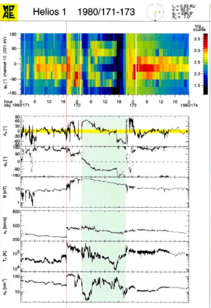
Fig. 3. The events associated with the interplanetary shock wave of 19 July 1980, as observed by the Helios 1 spaceprobe from a position at
0.53 AU distance to the Sun and at 92◦west of the Earth-Sun line, i.e. right above the Sun’s west limb as seen from the Earth. The 6 bottom panels show (from top) the IMF north-south (θB)and east-west (φB)direction, the field magnitude, and the solar wind speed, temperature
and density. The upper panel shows the azimuthal flow angle φEof suprathermal electrons (221 eV), with the anti-Sun direction at 0◦. This
is one of the cases for which Sheeley et al. (1985) could find a uniquely correlated CME. Figure courtesy of Kevin Ivory, MPS.
rising phase of solar activity. Since orientation and he-licity of filaments before eruption is often reflected in the topology of the resulting magnetic clouds (Both-mer and Schwenn, 1998; Yurchyshyn et al., 2001), we can use this knowledge for optimizing the prediction of geomagnetic effects (Zhao and Hoeksema, 1997, 1998; McAllister et al., 2001; Zhao et al., 2001).
Every CME launched with a speed exceeding 400 km/s was found to eventually drive a shock wave, which can be ob-served in-situ, provided that the observer is located within the angular span of the CME (Schwenn, 1983; Sheeley et al., 1983, 1985). In reverse, every shock wave observed in space (except the corotating ones) can uniquely be associated with
an appropriately pointed CME at the Sun. This implies that there is a causal chain linking CMEs to geomagnetic effects. No similar statement can be made for flares. Indeed, there are many CMEs (with geoeffects) without associated flares, and there are flares without associated CMEs (and without geoef-fects). The long-standing “flare myth” was finally abolished (see Gosling, 1993). However, for the very big and most dangerous events like the one Carrington happened to wit-ness, strong X-ray flares and large CMEs usually occur in a close timely context ( ˇSvestka, 2001). It is now commonly thought that both flares and CMEs are just the symptoms of a common underlying “magnetic disease” of the Sun (Harri-son, 2003).
1040 R. Schwenn et al.: The association of coronal mass ejections
Zhang et al. (2001, 2004) described the initiation of CMEs in a three-phase scenario: the initiation phase, the impulsive acceleration phase and the propagation phase. The initiation phase (taking some tens of minutes) always occurs before the onset of an associated flare, and the impulsive phase coin-cides well with the flare’s rise phase. The acceleration ceases with the peak of soft X-ray flares. Right at the launch time of several CMEs, Kaufmann et al. (2003) discovered rapid solar spikes at submillimeter wavelengths that might be represen-tative of an early signature of CME onset. In order to disen-tangle the various processes around CME initiation new ob-servations with significantly better resolution, both spatially and in time, and even supported by spectroscopic diagnos-tics, are needed, as was demonstrated by Innes et al. (2001) and Balmaceda et al. (2003). It is interesting to notice that some of the theoretical CME models begin to postulate dif-ferent phases of acceleration (see, e.g. Chen and Krall, 2003). Some authors claim that there are two kinds of coronal mass ejections (e.g. Sheeley et al., 1999; Srivastava et al., 2000, see also ˇSvestka, 2001; Moon et al., 2002): 1) grad-ual CMEs, with balloon-like shapes, accelerating slowly and over large distances to speeds in the range 300 to 600 km/s, and 2) Impulsive CMEs, often associated with flares, accel-erated already low down to extreme speeds (sometimes more than 2000 km/s). It is not yet clear whether these are re-ally fundamentre-ally different processes or whether they rep-resent just the extrema of an otherwise continuous spectrum of CME properties. These differences will be reflected in the properties of the related ICMEs and their effects. Tsurutani et al. (2004a) analyzed particularly slow magnetic clouds and found them to be surprisingly geoeffective. A good exam-ple is the famous event on 6 January 1997: A comparatively slow, unsuspiciously looking, faint partial halo CME caused a “problem storm” at the Earth 85 h later, with enormous ef-fects, as described in a series of papers (Zhao and Hoeksema, 1997; Burlaga et al., 1998; Webb et al., 1998). On the other hand, the very fast ICMEs are often found to be responsi-ble for the most intense geomagnetic storms (Srivastava and Venkatakrishnan, 2002; Gonzalez et al., 2004; Yurchyshyn et al., 2004), apparently because they build up extreme ram pressure on the Earth’s magnetosphere.
The number of CMEs observed at the Sun is about 3 per day at maximum solar activity (St.Cyr et al., 2000). Note though that Gopalswamy (2004) found a higher rate since their count included the extremely faint, narrow and slow CMEs that become visible due to the very high sensitivity and the enormous dynamic range of the LASCO instruments. The number of shocks passing an observer located, say, in front of the Earth, is about 0.3 per day (Webb and Howard, 1994). In other words, an observer sees only one out of ten shocks released at the Sun. The average shock shell covers about one-tenth of the full solid angle 4 Pi. Thus, the aver-age shock cone angle as seen from the Sun’s center amounts to about 100◦. This is significantly larger than the average angular size of the CMEs of about 45◦(Howard et al., 1985; Hundhausen, 1993; St.Cyr et al., 2000). The conclusion is that shock fronts extend much further out in space than their
drivers, the ejecta clouds, as had been suggested earlier by Borrini et al. (1982). This explains why a large fraction of shocks hitting the Earth are exhibiting just sheath plasma, with no ejecta following them. In any case, major geomag-netic storms may be driven.
These are all fairly empirical descriptions of the observed facts. However, the initiation and evolution of CMEs and the resulting propagation of the ejecta clouds through the he-liosphere have also been a key subject for theoreticians and modelers ever since. There is vast literature on various mod-els, some of them being quite controversial. The statement by Riley and Crooker (2004) describes the present status quite well: “These models include a rich variety of physics and have been quite successful in reproducing a wide range of observational signatures. However, as the level of sophis-tication increases, so does the difficulty in interpreting the results”. In fact, it is fair to say that at present there is not yet a unified understanding of all processes involved, and we are still searching for the decisive observational facts. For the response of the Earth’s system to those interplanetary pro-cesses the situation is not better. While the details of their in-teraction with the magnetosphere are still under study, some empirical relationships continue to be of great use, for ex-ample, the famous “Burton formula” (Burton et al., 1975, see also Lindsay et al., 1999a) that seems to be capable of predicting geomagnetic response from the sole knowledge of interplanetary parameters in front of the Earth.
3 Radial propagation of CMEs and travel time to 1 AU
In this section, we investigate how well the travel time of an ICME to an in-situ observer is related to the head-on CME speed near the Sun in the ideal case where both quantities can be precisely determined, for example, by a coronagraph near the Earth and an in-situ observer located at about 90◦offset in longitude relative to the Sun-Earth line.
Such favorable orbital constellations occurred in the later years of the Helios mission. The two Helios probes happened to cruise for substantial time periods near the plane of the sky (as seen from the Earth) at variables distances to the Sun (0.29 to 1 AU). Simultaneously, the SOLWIND coronagraph on the Earth-orbiting P78-1 satellite was watching many limb CMEs. Several of them were apparently aimed directly at Helios (see Schwenn, 1983; Sheeley et al., 1983). In 49 cases a unique association between SOLWIND limb CMEs and Helios in-situ ICMEs could be established (Fig. 3 shows one of these cases). The combined observations led to the conclusion that there is always a unique association between fast CMEs (faster than about 400 km/s) and in-situ shocks, provided the observer is located within the angular span of the CME (Schwenn, 1983; Sheeley et al., 1983, 1985). Fur-ther, every interplanetary shock (unless it is a corotating CIR shock) is the product of a CME. Sheeley et al. (1985) found only one shock without a discernible CME source. Note further that 2 of their 49 “safe” and 6 out of their 18 “pos-sible” associations involved CME and shock observations
R. Schwenn et al.: The association of coronal mass ejections 1041
above opposite limbs. This confirms that in extreme cases shock fronts can reach far around the Sun and thus disturb major parts of the whole heliosphere. For several of these events, Woo et al. (1985), using Doppler scintillation obser-vations, could show that substantial deceleration of shocks (with v>1000 km/s) takes place near the Sun and that the amount of deceleration increases with shock speed.
We have now revisited and extended these studies and cor-related the measured CME front speeds with the travel times of the associated shock waves to the Helios probe. Using the data listed in Table 1 of Sheeley et al. (1985), we derived the plot shown in Fig. 4 (unfortunately, expansion speeds were not measured at the time). For determining a “normalized” projected travel time to 1 AU we simply assumed that the shocks would travel from the Sun through Helios, all the way to 1 AU at the same average speed. The expected trend is clearly visible: the faster the CME, the shorter the travel time to Helios 1. But there is substantial scatter around the “ideal line”. While the fastest shocks arrive about as expected, the large group of very slow starters (<500 km/s) arrive substan-tially earlier than expected, and the majority of CMEs in the group 750 to 1000 km/s arrives later than expected. This con-firms generally what has been stated above (Gopalswamy, 2000, 2001c; Gonz´alez-Esparza et al., 2003a,b), that slow CMEs are post-accelerated by the ambient solar wind, and the fast ones are decelerated.
However, the large scatter in Fig. 4 comes as a surprise, and we cannot yet offer a unique explanation. The options are:
1. The CME speeds may not have been measured suffi-ciently well. This could be due to the low sensitivity of SOLWIND, its limited field-of-view (up to 10 Rs)
and to bad time cadence. In particular, the slow CMEs might be underestimated. We think that some of the data points in the slowest group should be shifted to-wards higher values of CME speeds.
2. Helios 1 was certainly not always hit by the fastest parts of the ICMEs. As shock fronts are large curved structures they will arrive later at observers situated in the ICME flanks, compared to the more frontal cases. For half of all interplanetary shocks no ejecta signa-tures were found by Helios, thus indicating flank passes
through the ICMEs. Thus, some travel time values
ought to be corrected towards smaller numbers.
3. The shock travel time must not be confused with the ejecta travel time. The ejecta follow their shocks a few hours later. Thus, the “real” ejecta travel times would be longer.
4. On their way through space, ICMEs travel through very different types of ambient solar wind. The solar wind conditions vary dramatically on short time scales as well as during the solar cycle. Thus, major deviations from simple kinematic models commonly used for predic-tions will occur.
4 0 500 1000 1500 2000 2500 3000 3500 0 20 40 60 80 100 120
Solwind CMEs-Helios shocks
travel time to 1 AU (h)
CME radial speed (km/s)
Figure 4. The travel time of limb CME fronts from the Sun to the location of Helios 1 (at about 900 off the Earth-Sun line) as function of the CME radial speed V
rad obtained from the
SOLWIND coronagraph. Only those cases were selected where a unique association could be achieved, in particular when Helios 1 was with +/- 300 near the plane of the sky, and when the
angular span of the CME included the Helios orbital plane. The travel time was derived from the moment of first appearance in a coronagraph image and the shock arrival time at Helios 1. The projected travel times to 1 AU as given in the figure were determined by simply assuming that the shocks would travel from the Sun through Helios and all the way to 1 AU at the same average speed . All data were adopted from Table 1 of Sheeley et al. (1985). The dotted line denotes the “ideal” line, i.e., where the travel time would exactly correspond to the CME radial speed near the Sun.
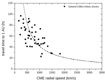
Fig. 4. The travel time of limb CME fronts from the Sun to the
location of Helios 1 (at about 90◦off the Earth-Sun line) as a func-tion of the CME radial speed Vrad obtained from the SOLWIND
coronagraph. Only those cases were selected where a unique as-sociation could be achieved, in particular when Helios 1 was with
±30◦near the plane of the sky, and when the angular span of the CME included the Helios orbital plane. The travel time was derived from the moment of first appearance in a coronagraph image and the shock arrival time at Helios 1. The projected travel times to 1 AU, as given in the figure, were determined by simply assuming that the shocks would travel from the Sun through Helios, all the way to 1 AU at the same average speed . All data were adopted from Table 1 of Sheeley et al. (1985). The dotted line denotes the “ideal” line, i.e. where the travel time would exactly correspond to the CME radial speed near the Sun.
Under 3) we encounter a pretty controversial issue (see Cane et al., 2000; Cane and Richardson, 2003b; and Gopal-swamy et al., 2003). It would of course be highly desirable and much more consistent if we could locate and then cor-relate identical features on both ends, i.e. in CME images and in in-situ data. This is what Gopalswamy et al. (2003) kept insisting on. But the driver gas often cannot be identi-fied uniquely or just misses the observer. Further, we can-not yet determine how the familiar three-part structure of most CMEs (bright outer loop, dark void, bright and struc-tured kernel (Hundhausen, 1988) is transformed into the fa-miliar two-part structure of ICMEs (sheath behind the shock wave, followed by driver gas/magnetic cloud) as illustrated in Fig. 3. Which is which? Before future work will solve this problem, we decided to put our present study on a purely em-pirical basis: we take the most uniquely observable quantities on both ends and look for correlations between them. Near the Sun, we take the first appearance in SOLWIND/LASCO-C2 images of the bright outer CME loop as reference time, and in space we look for any signs (including shocks) indi-cating approaching ICMEs. Note, by the way, that shocks are easily and uniquely detectable, in great contrast to the ejecta clouds.
If argument 4) is in fact a cause for the large scatter in Fig. 4, then we can already see that determining the radial
1042 R. Schwenn et al.: The association of coronal mass ejections
5
Figure 5. Self-similarity of CMEs: the limb CME of 19 October 1997 is a typical example showing how well the opening cone angle and the general shape of a CME are maintained, at least up to 32 Rs. The term “cone angle” denotes the angle between the outer edges of opposing
flanks of limb CMEs. It would amount to 650 in this case. The images are running differences
between LASCO-C3 images.
Fig. 5. Self-similarity of CMEs: the limb CME of 19 October 1997
is a typical example showing how well the opening cone angle and the general shape of a CME are maintained, at least up to 32 Rs.
The term “cone angle” denotes the angle between the outer edges of opposing flanks of limb CMEs. It would amount to 65◦in this case. The images are running differences between LASCO-C3 images.
6
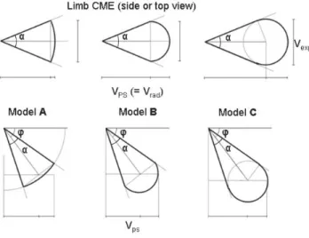
Figure 6. The drawings illustrate how the expansion speed Vexp is defined. It can be determined
uniquely for all types of CMEs, be it limb, partial halo or full halo CMEs, while the apparent plane of the sky speed VP S often contains an unknown speed component towards the observer.
6
Figure 6. The drawings illustrate how the expansion speed Vexp is defined. It can be determined
uniquely for all types of CMEs, be it limb, partial halo or full halo CMEs, while the apparent
plane of the sky speed VP S often contains an unknown speed component towards the observer.
Fig. 6. The drawings illustrate how the expansion speed Vexpis
defined. It can be determined uniquely for all types of CMEs, be it limb, partial halo or full halo CMEs, while the apparent plane of the sky speed VP S often contains an unknown speed component
towards the observer.
CME speed near the Sun alone will not guarantee good pre-dictions. The propagation conditions have to be taken into account as well.
As a conclusion of this section we note:
– There is indeed a correlation between the radial front
speed Vrad of limb CMEs and the travel time towards
an in-situ observer.
– Slow CMEs are post-accelerated, fast ones are
deceler-ated.
– The scatter is surprisingly high.
7 0 500 1000 1500 2000 0 200 400 600 800 1000 1200 1400 1600 1800 2000
less than 80 deg. between 80 and 120 deg. more than 120 deg.
expansion speed (km/s)
radial speed (km/s)
Figure 7. The correlation between radial CME speed Vrad and the lateral expansion speed Vexp for
limb CMEs observed by LASCO between January 1997 and April 15, 2001.
Fig. 7. The correlation between radial CME speed Vrad and the lateral expansion speed Vexpfor limb CMEs observed by LASCO
between January 1997 and 15 April 2001.
4 The expansion speed serves as proxy for the radial propagation speed of CMEs
Now we will study a number of limb CMEs observed by LASCO where the radial speed Vrad (which in these is
iden-tical to VP S)and the expansion speed Vexp could both be
measured, in order to check the value of the latter one as proxy data for the other one. Upon inspecting many hun-dreds of CMEs observed from SOHO we confirmed the ob-servation by Plunkett et al. (1998) that for limb events the cone angles of expansion and, more generally, the shapes of the expanding CMEs were strikingly maintained (by the term “cone angle” we mean the angle between the outer edges of opposing flanks of limb CMEs). The CME shapes remained “self-similar” throughout the LASCO field-of-view. In other words, the ratio between lateral expansion and radial prop-agation appears to be constant for most CMEs. A typical example is shown in Fig. 5.
The way of determining the radial speed Vrad and the
ex-pansion Vexp speed of a CME is illustrated in Fig. 6 (from
Dal Lago et al., 2003a). We selected a representative sub-set of limb CMEs (57 in total), where EIT images showed a uniquely associated erupting feature within 30◦in longitude
to the solar limb and within a reasonable time window of a few hours. Further, sufficient coverage in C3 images was re-quired. For those events we determined both the radial speed Vrad (of the fastest feature projected onto the plane of the
sky) and the expansion speed Vexp(measured across the full
CME in the direction perpendicular to Vrad). We measured
them when they had reached constant values, i.e. usually at around 10 Rs.
Figure 7 shows the result: There is indeed a fairly good correlation between the two quantities. A linear fit through the data yields
with a correlation coefficient of 0.86. Apparently, the corre-lation shown in Fig. 7 holds for the slow CMEs as well as for the fast ones, for the narrow ones as well as for the wide ones. The correlation even holds in the extreme cases where a cloud expands faster than it moves as a whole; the front motion would then mainly be due to the expansion alone, where the cone angle amounts to 180◦ and Vrad would be
about equal to Vexp, in fairly good agreement with Eq. (1).
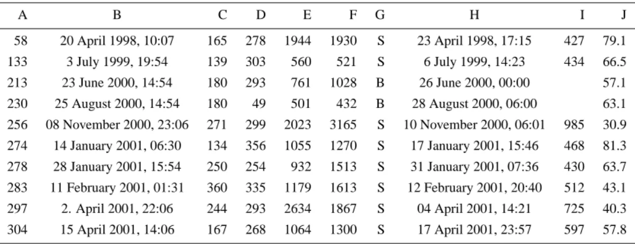
As an example the limb CME of 20 April 1998, shown in Fig. 8, can be considered: This was an extremely fast event right behind the west limb with Vrad=1944 km/s and
Vexp=1930 km/s and a cone angle of 170◦. In fact, the
ef-fects from this extraordinary limb event even hit the Earth 79.1 h later and caused a moderate geomagnetic storm (Dst
−59 nT).
In order to understand this remarkable correlation we tried
some modeling of CME evolution. We assumed various
plausible geometries based on the “ice cream cone model”, as first described by Fisher and Munro (1984) and applied again, e.g. by Zhao et al. (2002) and Michalek et al. (2003). We modeled the CME front surface as a section of an expand-ing sphere and calculated the ratio Vexp/Vrad as a function
of the cone angle α. Figure 9 (upper panels) illustrates the 3 geometries we used: the front sphere could either be a sphere section with the Sun in the center (Model A), or a half sphere sitting on top of a cone (Model B), or a sphere dropped into a cone (like a real ice cream ball, such that the ball surface touches the sphere tangentially, Model C). We assumed the cone angle to be constant and the sphere surface to remain self-similar throughout the expansion. It turns out that in the cone angle range from 40◦to 80◦, where most CMEs belong,
model A yields Vexp/Vradfrom 1.2 to 0.85, compared to the
experimental value of 0.88. The other models give slightly higher values. On the other hand, for a cone angle near 180◦ Model C works best. One can easily verify that for this ge-ometry model C yields Vexp=Vrad (see also the example of
Fig. 8). In view of the rather crude assumptions about CMEs’ shape and evolution this is not a bad agreement between our finding and the models.
We further extended these models to cases where the CMEs are pointed away from the plane of the sky by an angle φ(see Fig. 9, lower panels). We calculated the values for the apparent VP Swhich now no longer equals Vradas it does for
limb CMEs. However, unless φ becomes larger than the cone angle α, VP Sand Vrad remain equal or almost equal, in any
model. When φ approaches 90◦, i.e. for the central halo
con-stellation, all 3 models converge to VP S=Vexp/2, regardless
of the cone angle, as expected. In other words, for a given CME the apparent VP S value varies substantially with the
viewing angle φ, while the Vexpvalue does not. This is why
Vexpis superior to VP S for inferring the radial speed Vrad
of halo CMEs.
After all we can state:
– For limb CMEs the radial front speed Vradis almost the
same as the expansion speed Vexp.
8
Figure 8. The extremely fast partial halo limb CME of 20 April 1998 (E58) was associated with a M1.6 flare not far behind the west limb. The images are running differences between LASCO
C3 images. The expansion angle was about 1800. The expansion speed was 1930 km/s, the plane
of the sky speed was 1944 km/s. A shock arrived at the Earth 79.1 hours later, i.e., about 24 hours
later than we predicted. A moderate magnetic storm (Dst –59 nT) peaked 13 hours after shock
arrival.
Fig. 8. The extremely fast partial halo limb CME of 20 April 1998
(E58) was associated with a M1.6 flare not far behind the west limb. The images are running differences between LASCO C3 images. The expansion angle was about 180◦. The expansion speed was 1930 km/s; the plane of the sky speed was 1944 km/s. A shock ar-rived at the Earth 79.1 h later, i.e. about 24 h later than we predicted. A moderate magnetic storm (Dst −59 nT) peaked 13 h after shock
arrival.
9
Figure 9. 3 plausible models of CME geometries used for stud ying the ratio between Vexp and Vrad and their relation to the plane of the sky speed VPS. The front surface is assumed to be a sphere section, either with the Sun in the center (A), or a half sphere sitting on top of a cone (B), or a sphere dropped into a cone (like a real ice cream ball, such that the ball surface touches the sphere tangentially, C). The cone angle a (i.e., the full angle between between the outer edges of opposing flanks of CMEs) and the radial speed Vrad are assumed to be constant with time. Thus, the linear dimensions are proportional to the speeds Vexp and Vrad. The upper panels apply to limb CMEs, viewed from the top or from the side. For the lower panels, the CMEs are off-pointed by an angle f with respect to the plane of the sky.
Fig. 9. Three plausible models of CME geometries used for
study-ing the ratio between Vexpand Vradand their relation to the plane
of the sky speed VP S. The front surface is assumed to be a sphere
section, either with the Sun in the center (A), or a half sphere sitting on top of a cone (B), or a sphere dropped into a cone (like a real ice cream ball, such that the ball surface touches the sphere tangen-tially, C). The cone angle α (i.e. the full angle between between the outer edges of opposing flanks of CMEs) and the radial speed Vrad
are assumed to be constant with time. Thus, the linear dimensions are proportional to the speeds Vexpand Vrad. The upper panels
apply to limb CMEs, viewed from the top or from the side. For the lower panels, the CMEs are off-pointed by an angle φ with respect to the plane of the sky.
– The plane of the sky speed VP S can differ from Vexp
and the wanted Vrad value by a factor of 2, depending
on the CME direction.
– The expansion speed Vexpis a fairly reliable proxy for
1044 R. Schwenn et al.: The association of coronal mass ejections
5 The evaluation of halo CMEs near the Sun and ICMEs near the Earth
We searched the LASCO data from January 1997 to 15 April 2001 for all CMEs that might be considered candidates for producing effects near the Earth, i.e. halo and partial halos. Independently, we searched all in-situ data obtained near the Earth for signatures of ICMEs.
5.1 CMEs observed near the Sun
All LASCO data were searched for full or partial halo CMEs. Visual inspection was required since automated recogni-tion schemes that are under prepararecogni-tion (e.g. Robbrecht and Berghmans, 2004) are not yet available. A CME is termed a “full” halo if a feature (remember the CME definition) ap-pears in at least one image all around the occultor. A “partial” halo has an angular span of at least 120◦. The distinction be-tween full and partial halos often suffers from the fact that the CME brightness and structure vary strongly with the position angle. The features we see might be the ejecta themselves, or the compressed and deflected material related to a shock out ahead of the CME, or the superposition of 2 or more separate CMEs.
We included all these events in the study since they might have a significant speed component along the Sun-Earth-line and may thus be relevant for space weather issues. In the remainder of this paper, the term “halo” will always mean both: full and partial halos. Typical examples for the CME types are shown in Fig. 6. For the search, we inspected the reports issued by the LASCO operations team at GSFC un-der ftp://ares.nrl.navy.mil/pub/lasco/halo. They helped us to avoid overlooking some of the fainter CMEs, and they gave us important information on the halos’ first appearance in C2 images, apparent direction, plane-of-the-sky speed, and correlations with disk events as seen by EIT. This latter in-formation, in particular, allowed us to earmark off-pointed (backside) CMEs early on. Further, we studied the CME cat-alog under http://cdaw.gsfc.nasa.gov/CME list/. In order to clarify differences between the catalogs and to derive unique and consistent evaluations, we inspected ourselves every sin-gle CME image sequence. This explains why in some cases we arrived at different interpretations.
Table 1 gives the numbers of front side halos (F), backside halos (B), limb CMEs (L) and unclear cases (U) where we could not decide about the source location. The limb events are those with an apparent eruption within 30◦ of the limb
of the front side disk. The unclear cases are those where we could not uniquely determine whether the halos were front-or backside events. Note that the numbers of backside ha-los is not representative anyway, since more such events oc-curred but were not registered and evaluated in the context of this paper. We skipped some of the events listed as halos in the http://cdaw.gsfc.nasa.gov/CME list/ catalog because they were so faint that we could not confirm them ourselves, even when we applied our most sophisticated technique as described by Dal Lago et al. (2003b). The column “Other”
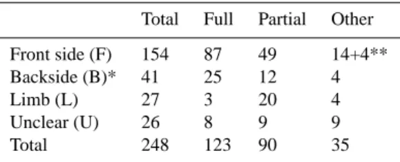
Table 1. Summary of all halo CME observations by LASCO from
January 1997 to 15 April 2001.
Total Full Partial Other Front side (F) 154 87 49 14+4** Backside (B)* 41 25 12 4 Limb (L) 27 3 20 4 Unclear (U) 26 8 9 9 Total 248 123 90 35
* The numbers for backside events are not representative.
* For those 4 cases the CME identification was done with instru-ments other than SOHO, e.g. the Nanc¸ay radioheliograph, or the GOES satellites.
events addresses CMEs that we considered relevant although their angular width was less than 120◦. Their importance in context with this work showed up later. Further, there are 4 more “other” cases were SOHO data were not available, but there are other good reasons to classify them as full front side halo CMEs.
For each event we determined the characteristic data and noted them in our data bank (interested readers are referred to the webpage http://star.mpae.gwdg.de/cme effects/). After all, we recorded a total of 248 relevant CME events that oc-curred in the time period between January 1997 and 15 April 2001. Neglecting the 41 backside and 26 unclear events, we ended up with a total of 181 CME candidates for further anal-ysis. The list of 181 relevant CMEs includes 18 non-halo CMEs, i.e. CMEs with an extension of less than 120◦ and the 4 front side CMEs for which there exist no SOHO data. The actual relevance of these events for this study was dis-covered from other sources.
For each CME event we evaluated and listed in the data bank the following entries:
– The time of first appearance in C2 is taken as
refer-ence onset time, for practical reasons: the actual on-set is not always uniquely discernible in data from EIT or Yohkoh, because there is often too much activity around. Experience tells us that only those events that make it into the C2 field-of-view become relevant for our study. The time difference between the CME onset in EIT and its appearance in C2 is of the order of one hour, i.e. small compared to the travel times to 1 AU of some 80 h.
– The position angle and angular extent values we copied
(after inspection) from the catalog http://cdaw.gsfc. nasa.gov/CME list/.
– The plane of the sky speed VP Svalues were also copied
from the same catalog (the linear fit speed values). Note that they were derived for the fastest feature in the im-ages sequences (St.Cyr et al., 2000). The time-height diagrams usually show an increasing speed in the C2 field-of-view, but in the C3 field the speeds appear to be
constant from about 10 Rson. In cases where a linear fit
obviously does not work, we chose the second order fit at 20 Rs. If C3 data were not available, we inserted the
C2 value with a minus sign added as an earmark.
– The expansion speed Vexpwas determined according to
Fig. 6. Usually, halos appear with more or less ellip-tical cross sections. Even a CME with a perfectly cir-cular cross section would exhibit an elliptical shape if it is not pointed exactly along the Earth-Sun line. This is why Vexp has to be determined from the expansion
of the brightest and fastest features perpendicular to the projected propagation direction. We plotted the lateral expansion as a function of time (similar to a height time plot) and derived a value for Vexpwhen it had reached
a constant value, i.e. for halo widths of some 15 Rs.
5.2 ICMEs recorded by spacecraft in front of the Earth
In order to study the potential correlations between CMEs and their effects on the Earth, we searched for the arrival signatures of ICMEs at the location in front of the Earth’s bow shock, i.e. at the SOHO, WIND or ACE spacecraft, all cruising around the L1 point.
What is the optimum ICME signature? In about half of all cases, the ejecta themselves do not hit the Earth, although their associated shocks may drive substantial geomagnetic storms (Gosling et al., 1991), and even if so, the ejecta are often not uniquely discernible. Some authors (e.g. Gopal-swamy et al., 2000) used magnetic cloud signatures and low plasma beta as markers. These signatures appear not to be unique, and many events will probably be missed. In other studies, the onset times of geomagnetic storms or the Dst
peak times were taken as further markers (e.g. Brueckner et al., 1998; Zhang et al., 2003). We do not consider this to be a very appropriate method, since a storm may be caused either by the sheath plasma ahead of the ejecta or hours later by the ejecta themselves, or by a combination of both, or even not at all. For those cases where it could be determined, the de-lay time between ICME arrival and Dst peak time was found
to vary between 3 and 40 h, with an average value of 18 h (Russell and Mulligan, 2002; Zhang et al., 2003).
What suffers least from such shortcomings is the shock signature as seen in plasma and IMF data taken outside the Earth’s bow shock. This signature sticks out so clearly that it can hardly be overlooked or misinterpreted. Even a computer can be taught to identify shocks (e.g. http://umtof.umd.edu/ pm/shockspotter.html).
Of course are we aware of the fact that transient shocks are NOT parts of the ICMEs themselves. It is true that shocks are driven by ICMEs, but they move within the ambient solar wind, which determines their propagation properties. These properties vary dramatically from event to event, due to the 3-D structure of the solar wind streams and the IMF. On the other hand, as shown above, the correlation between fast CMEs and the occurrence of interplanetary shocks is safely established (Schwenn, 1983; Sheeley et al., 1985).
Our intention here is to derive an empirical tool based on the most unique available signatures on both ends: the CMEs observed early on by coronagraphs, and the ICME signa-tures observed in front of the Earth. Therefore, we searched through all in-situ plasma and field data that are available on the Web. They are provided by the SWE and MFI in-struments on the WIND spacecraft, by the SWEPAM and MAG instruments on the ACE spacecraft, and by the MTOF-CELIAS proton monitor on SOHO. This way, a 100% com-plete data coverage over the study interval from January 1997 to 15 April 2001 could be achieved.
The occurrence of a shock wave can be recognized in in-situ plasma data by a noticeable, abrupt, and simultaneous increase of speed, density, temperature, and magnetic field magnitude (see Fig. 3). “Abrupt” means between adjacent data points, usually taken a few seconds or minutes apart. The knowledge of the magnetic field increase is considered mandatory.
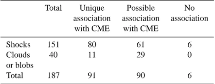
By visual inspection using these criteria a total of 147 shocks were identified, (plus 4 CIR shocks in front of coro-tating high-speed streams).
For each shock we made these entries in a shock catalog:
– the time of arrival, preferentially from ACE data, – the solar wind speed and density values on both sides of
the shock that allowed calculating a rough local shock speed Vshaccording to Eq. (6.6) in Hundhausen (1972).
Recognizing ejecta not accompanied by shocks is not uniquely possible. The signatures are too hard to discern. Occasionally, a trained eye may discover a candidate event by chance, or triggered by a halo alarm issued, for exam-ple, by the LASCO operations team (see http://lasco-www. nrl.navy.mil/halocme.html). Huttunen et al. (2002) show a good example (our case E7) in their Fig. 2. We inserted 40 such events into our catalog: 22 of them we regard as prob-able magnetic clouds (M events) and 18 others as suspicious density blobs (B events) without magnetic cloud signature. We do not consider that list complete or in any sense rep-resentative, since no systematic search could be performed because of the severe ambiguities.
During this search, we noted other quantities for future use, for example, certain ICME signatures, and the Kp and
Dst values of associated geomagnetic storms, if applicable.
This lead us to include all at least moderate geomagnetic storm events, i.e. when Dst fell below −50 nT, regardless
of shock occurrence (as one of the referees pointed out, one should use the change of Dst relative to pre-storm levels for
storm strength definition rather than the absolute values. We will do that in succeeding papers when the storm effects will be primarily studied). This way, the major geoefficient mag-netic clouds were located, plus another 4 geoeffective CIRs without corotating shocks.
We compared our list with the various lists compiled by other authors and found ourselves in a big mess. To illus-trate the problem, let us mention only one example: Cane and Richardson (2003a) studied an overlapping time period (May