Assessing uncertainty in radar measurements on simplified meteorological scenarios

(1)

HAL Id: hal-00296868

https://hal.archives-ouvertes.fr/hal-00296868

Submitted on 20 Feb 2006

HAL is a multi-disciplinary open access

archive for the deposit and dissemination of

sci-entific research documents, whether they are

pub-lished or not. The documents may come from

teaching and research institutions in France or

abroad, or from public or private research centers.

L’archive ouverte pluridisciplinaire HAL, est

destinée au dépôt et à la diffusion de documents

scientifiques de niveau recherche, publiés ou non,

émanant des établissements d’enseignement et de

recherche français ou étrangers, des laboratoires

publics ou privés.

Assessing uncertainty in radar measurements on

simplified meteorological scenarios

L. Molini, A. Parodi, N. Rebora, F. Siccardi

To cite this version:

L. Molini, A. Parodi, N. Rebora, F. Siccardi. Assessing uncertainty in radar measurements on

sim-plified meteorological scenarios. Advances in Geosciences, European Geosciences Union, 2006, 7,

pp.141-146. �hal-00296868�

(2)

SRef-ID: 1680-7359/adgeo/2006-7-141 European Geosciences Union

Advances in

Geosciences

Assessing uncertainty in radar measurements on simplified

meteorological scenarios

L. Molini, A. Parodi, N. Rebora, and F. Siccardi

CIMA, University of Genoa, Savona, Italy

Received: 11 November 2005 – Revised: 25 December 2005 – Accepted: 16 January 2006 – Published: 20 February 2006

Abstract. A three-dimensional radar simulator model (RSM) developed by Haase (1998) is coupled with the non-hydrostatic mesoscale weather forecast model Lokal-Modell (LM). The radar simulator is able to model reflectivity mea-surements by using the following meteorological fields, gen-erated by Lokal Modell, as inputs: temperature, pressure, water vapour content, cloud water content, cloud ice content, rain sedimentation flux and snow sedimentation flux. This work focuses on the assessment of some uncertainty sources associated with radar measurements:

1. absorption by the atmospheric gases, e.g., molecular oxygen, water vapour, and nitrogen;

2. attenuation due to the presence of a highly reflecting structure between the radar and a “target structure”. RSM results for a simplified meteorological scenario, con-sisting of a humid updraft on a flat surface and four cells placed around it, are presented.

1 Introduction

The use of weather radars is relevant for both precipitation rate retrieval and data assimilation purposes because of their capability to provide measures of dynamical and microphys-ical states at high temporal and spatial resolution. Nev-ertheless, a wide range of uncertainty sources affect radar measurements and their products, challenging their reliabil-ity. Since early 90s, numerical simulations of radar mea-surements have provided a suitable tool to investigate some of the main aspects of this issue. For instance, a complex work on influence of drop size distribution and X-band at-tenuation on reflectivity was carried out by Chandrasekar and Bringi (1990), the importance of measurement volume vari-ations depending on increasing radar distance has been as-sessed by Fabry et al. (1992), uncertainty due to empirical Correspondence to: L. Molini

(luca.m@cima.unige.it)

Z-R relations has been analysed by Krajewski and Anagnos-tou (1997) and bright band effects on reflectivity were stud-ied by Skaropoulos and Russchenberg (2002). Krajewski and Chandrasekar (1993) simulated radar reflectivity for realistic rainfall events using a stochastic space-time model for pre-cipitation and a statistically generated drop size distribution (DSD), while Haase and Crewell (2001) used the three di-mensional fields of atmospheric variables generated by a nu-merical weather prediction model (see also Keil and Hagen, 2000; Meetschen and Crewell, 2000).

In order to assess some basic uncertainty sources (like gaseous absorption and screening effect of a precipitating structure located between the radar and a “target” structure), the latter approach is followed. A simplified atmospheric scenario is generated by the Lokal-Modell (LM) and stan-dard radar products like plan position indicator (PPI) and range height indicator (RHI) scans have been simulated by RSM. Simulations have been performed either considering uncertainty sources or not taking these factors into account so as to compare data and gain an assessment of their influ-ence on radar measurements. This work is organized as fol-lows: Sects. 2 and 3 give a brief overview of Lokal-Modell and Radar Simulation Model, Sect. 4 shows simulation re-sults and quantitative analysis on them and finally, Sect. 5 contains conclusion and future outlooks.

2 The Lokal-Modell

The numerical simulations shown in this work have been per-formed with Lokal-Modell which is a non-hydrostatic nu-merical weather prediction model developed by Deutsche Wetterdienst (DWD, the German National Weather Service) since 1998 (Doms and Sch¨attler, 1998); it is fully com-pressible, using hybrid terrain-following coordinates, hav-ing a maximum horizontal spatial resolution of 50 km, while the vertical resolution may vary from a value of 50 m near surface up to several hundred metres with increasing alti-tude. The basic prognostic model variables are wind vector,

(3)

142 L. Molini et al.: Assessing uncertainty in radar measurements

temperature, pressure perturbation, specific humidity and cloud liquid water, while rain and snow fluxes are diagnostic variables. Lokal-Modell can use a wide range of microphys-ical schemes spacing from the Kessler (warm rain) scheme to the 3-category ice scheme. For a more comprehensive de-scription of the model, the reader is referred to Steppeler et al. (2003).

In this work we operate:

– a 1 km horizontal spacing grid

– a regularly spaced vertical grid (1z=200 m)

– a 2 category ice scheme which can model 5

microphys-ical species: rain, snow, cloud water, cloud ice, water vapour and the microphysical processes related to.

3 The Radar Simulator Model

The Radar Simulator Model (RSM) is able to simulate the most important atmospheric interactions of an electromag-netic wave with hydrometeors, e.g. backscattering and at-tenuation. In order to calculate the volume backscattering and extinction cross sections, some of the three-dimensional fields of Lokal-Modell outputs are required:

1. rain sedimentation flux [kg/m−2s] 2. snow sedimentation flux [kg/m−2s] 3. temperature [K]

4. pressure [Pa]

5. cloud ice specific content [kg/kg] 6. cloud water specific content [kg/kg] 7. water vapour ratio [kg/kg]

The second step consists of applying the Mie scattering the-ory (Mie, 1908) by which

κ = λ 3 8π2 ∞ Z 0 χ2N (χ ) ξ (χ ) dχ (1) where:

– κ represents the volume absorption, scattering or

extinc-tion coefficient depending on which efficiency factor ξ (absorption, scattering or extinction) is inserted in the integrand

– χ =2π /λ is the dimensionless shape factor – N (χ ) represents the drop size distribution (DSD)

While rain and snow are assumed to have exponential DSDs in the LM (Marshall-Palmer, 1949 and Gunn-Marshall, re-spectively), a cloud DSD is not resolved: therefore RSM de-fines a DSD for cloud liquid water taking a cumulus or a

cirrostratus DSD from literature (Chylek and Ramaswamy, 1982 for cloud water and Ulaby et al., 1981 for cloud ice). The calculation of extinction cross section is performed by using the millimeter-wave propagation model from Liebe et al. (1989) which allows to consider the effects of absorption by atmospheric gases (e.g., molecular oxygen, water vapour and nitrogen). When all the contributions to the total ex-tinction cross section have been calculated, the backscattered power from the scanned volume to the radar can be expressed as follows Pr =Crad 1 R4Vpκbackexp  −2 R Z 0 κextdR   (2) where:

– Crad [m2] is the radar constant

– R [m] is the range to the scattering volume – Vp[m3] is the pulse volume at range R.

A relation between received power and reflectivity factor was determined by assuming only liquid particles (an equivalent radius is calculated for snow) and pure Rayleigh scattering:

Pr =Crad 1 R4Vp10 −10π5 λ4 |K| 2_Z ₍₃₎ where:

– |K|2=0.93 is the dimensionless refraction constant for water

– λ is the wavelength [cm].

Considering both Eqs. (2) and (3) leads to the form below:

Zsim=1010 λ4 π5κbackexp  −2 R Z 0 κextdR   (4)

Commonly, radar reflectivity is measured in dBZ=10log10

(Z).

RSM output consists of simulated PPI or RHI scans which actually consider radar beam geometry (and its effects on measurements) Moreover, RSM can calculate a reflectivity value for each domain grid point (reflectivity volume), just by summing up the contribution of each microphysical species without considering any physical interference to the measure. In practice, the true reflectivity value for each grid point is provided.

4 Numerical experiments

The characterization of uncertainty in radar measurements is addressed by using, as atmospheric target scenario, a system of deep convective structures over an aquaplanet. The nu-merical simulations are initialized considering a horizontally homogeneous atmosphere in which we locate:

(4)

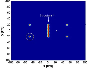
Fig. 1. Horizontal section of initial temperature 3-D field at 100 m

quota. The dotted circle marks the “target cell”, while the white triangle shows the radar position.

– STRUCTURE 1: an ascending current of humid air,

whose volume is 10×40×1 km, centred on domain mean section, warmer (1Tmax=1 K) than the

environ-ment.

– STRUCTURES 2-3-4-5: four axially symmetric

ther-mal perturbations (warm bubbles) of vertical radius 1000 m and horizontal radius 10 km. The amplitude of the temperature perturbation is maximum in the cell’s centre (1 K) and gradually decreases on approaching the bubble boundaries.

Both kind of structures were used so as to trigger deep moist convection generating high intensity precipitating struc-tures. Figure 1 shows that the computational domain size is 200×200×20 km, having the same horizontal (1 km) and vertical (200 m) resolution features mentioned in Sect. 2. Finer resolution experiments will be carried out later on. The vertical profile of temperature and humidity inside the com-putational domain are defined according to Weisman and Klemp (1982, 1984), corresponding to convective available potential energy of about 3000 J/kg, while neither wind shear nor orography effects are taken into account.

4.1 First experiment–gaseous (nitrogen, molecular oxygen, water vapour) absorption effect

To point out only the effects of gaseous absorption, the pres-ence of the ascending current between radar and the selected target cell is not considered. In this first test, we compare:

1. horizontal and vertical sections of the reflectivity vol-ume (see Sect. 3) after regridding them on the same po-lar grid of PPI and RHI scans, respectively.

2. both PPI and RHI scans of RSM obtained by taking into account the geometry of the radar beam

Fig. 2. Vertical section of the volume reflectivity regridded on the

RHI scan polar grid: the “target cell”.

Fig. 3. RHI scan of the target cell. Maximum elevation angle: 30◦.

In other words, Fig. 2 shows what we should see if we could be able to perform “perfect” radar scans measuring reflec-tivity for each domain grid point without any atmospheric interference. Dotted white circles in Fig. 3 show the regions where radar signal loss is more evident. Then, Fig. 4 dis-plays the vertical reflectivity profile of both regridded vol-ume and RHI scan. The mean difference is about 5 dBZ (45 vs 40 dBZ) which means 24 vs 12 mm/h in terms of pre-cipitation rate, using Marshall-Palmer (1948) relation. Very similar results have been found by performing comparisons between PPI scans and horizontal regridded sections of the reflectivity volume.

4.2 Second experiment – screening effect

The second experiment is devoted to measuring the screen-ing effects of an intense precipitatscreen-ing structure located (i.e. Structure 1) between the radar and the target cell: in order to retrieve differences, PPI and RHI scans are performed, in which alternately:

(5)

Fig. 4. Vertical profile of reflectivity: green dotted line represents

the RHI scan while the purple dotted line indicates the regridded volume section.

Fig. 5. The “target cell” viewed under a 5◦elevation-PPI scan: the screening effect is taken into account, while an intensely reflecting core can be seen in the left region of the cell.

1. Structure 1 is taken into account 2. Structure 1 is not considered

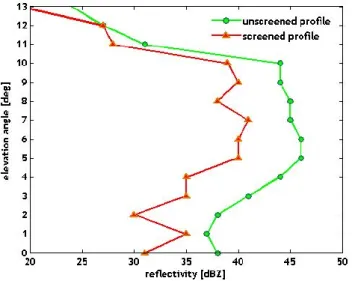
The difference between unscreened and screened PPI is dis-played in Figs. 5, 6 and 7: despite that the cell shape is well conserved, the more intense core and the southern side appear (the farther from radar site) largely underestimated. Figure 8 shows the main differences between the two data sets in terms of maximum reflectivity (59 vs 53 dBZ), mean reflectivity (39 vs 28) and standard deviation (8 vs 9 dBZ). The vertical reflectivity of the screened cell and of the un-screened one are shown in Fig. 9, while Fig. 10 illustrates the mean reflectivity vertical profile of Structure 1 and the vertical mean difference between an unscreened RHI versus a screened one. Major differences, depending not only on higher reflectivity values of Structure 1 (i.e. a higher rate of

Fig. 6. Again, the “target cell” reflectivity is shown but no screening

effect is now considered.

Fig. 7. Difference between unscreened and screened target cell.

screened radiation) but also on screening structure thickness, can be noticed.

5 Conclusions

In this work, preliminary results obtained by using Lokal-Modell/RSM chain in simplified atmospheric scenarios are presented. The first experiment was to check RSM capability to reproduce reliably some of the physical problems affect-ing radar measurements like signal power loss by gaseous absorption (nitrate, molecular oxygen, water vapour) and to quantify its influence on reflectivity measures. The second experiment has been developed so as to determine how and how much a screening effect induced by an intensely pre-cipitating structure could affect radar measures on a target structure.

Future work will be spent in analysing other uncertainty sources like the use of different radar bands (X band and S band) and, most of all, the use of both different microphysi-cal schemes (the 3-category ice scheme) and different DSDs (Sekhon and Srivastava, 1971; Douglas, 1964; Feingold and Levin, 1986; Ulbrich, 1983) to model atmospheric processes.

(6)

Fig. 8. Maximum reflectivity, mean reflectivity and standard

devia-tion of both unscreened and screened cell.

Fig. 9. Vertical profiles of screened cell (red line) and unscreened

cell (green line).

Edited by: V. Kotroni and K. Lagouvardos Reviewed by: S. Michaelides

References

Chandrasekar, V. and Bringi, V. N.: Error Structure of Multiparam-eter radar And Surface Measurements of Rainfall Part III: Spe-cific Differential Phase, J. Atmos. Oceanogr. Technol., 7, 621– 629,1990.

Chylek, P. and Ramaswamy, V.: Simple approximation for infrared emissivity of water clous, J. Atmos. Sci., 39, 171–177, 1982. Douglas, R. H.: Hail size distribution, paper presented at 1964

World Conference on Radar Meteorology, American Meteoro-logical Society, Boulder, Colorado, 1964.

Doms, G. and Sch¨attler, U.: The nonhydrostatic limited-area model LM (Lokal-Modell) of DWD, part I, Scientific Documentation, 1998.

Fig. 10. Mean reflectivity vertical profile of screening structure and

mean vertical difference of the target cell.

Fabry, F., Austin, G. L., and Tees, D.: The accuracy of rainfall es-timates by radar as a function of range, Q. J. R. Meteorol. Soc., 118, 435–453, 1992.

Feingold, G. and Levin, Z.: The lognormal fit to raindrop spectra from frontal convective clouds in Israel, J. Climate Appl. Me-teor., 25, 1346–1363, 1986.

Gunn, K. L. S. and Marshall, J. S.: The distribution with size of aggregate snowflakes, J. Meteorol., 15, 452–461, 1958

Haase, G.: Simulation von Radarmessungen mit Daten des Lokalmodells, Diplomarbeit in Meteorologie vorgelegt, 1998. Haase, G. and Crewell, S.: Simulation of radar reflectivities

us-ing a mesoscale weather forecast model, Water Resour. Res., 36, 2221–2231, 2001.

Keil, C. and Hagen, M.: Evaluation of high resolution NWP simula-tions with radar data, Phys. Chem. Earth, 25, 1267–1272, 2000. Krajewski, W. and Chandrasekar, V.: Physically Based Radar

Sim-ulation of Radar Rainfall Data Using A Space Time Rainfall Model, J. Appl. Meteorol., 32, 268–283, 1993.

Krajewski, W. and Anagnostou, E.: Simulation of radar reflectiv-ity fields: Algorithm formulation and evaluation, Water Resour. Res., 33, 1419–1428, 1997.

Liebe, H. J.: MPM-An atmospheric millimeter-wave propagation model, Int. J. Infrared and Millimeter Waves, 10, 631–650, 1989. Marshall, J. S. and Palmer, W. M.: The distribution of raindrops

with size, J. Meteorol., 5, 165–166, 1948.

Meetschen, D. and Crewell, S.: Simulation of weather radar prod-ucts from a mesoscale model, Phys. Chem. Earth, 25, 1257– 1261, 2000.

Mie, G. : Beitr¨age zur Optik tr¨uber Medien, Ann. Physik, 25, 377– 445, 1908.

Sekhon, R. S. and Srivastava, R. C.: Doppler radar observations of drop-size distributions in a thunderstorm, J. Atmos. Sci., 28, 983–994, 1971.

Skaropoulos, N. and Russchenberg, W.: A model of radar backscat-tering from the melting layer of precipitation, Proceedings of ERAD 2002, 2002.

Steppeler, J., Hess, R., Doms, G., Sch¨attler, U., and Bonaventura, L: Review of numerical methods for non hydrostatic weather pre-diction models; Meteorol. Atmos. Phys., 82, 287–301, 2003.

(7)

Ulaby, F. T., Moore, R. K., and Fung, A. K.: Microwave remote Sensing, Active and passive, Addison-Wesley-Longman, Read-ing, Mass., 1, 456 pp., 1981.

Ulbrich, C. W.: Natural variations in the analytical form of the raindrop size distribution, J. Climate Appl. Meteorol., 22, 1764– 1775, 1983.

Weisman, M. and Klemp, J.: The dependence of the numerically simulated convective storms on wind vertical shear and buoy-ancy, Mon. Wea. Rev., 110, 504–521, 1982.

Weisman, M. and Klemp, J.: The structure and classifications of numerically simulated convective storms in directional varying wind shears, Mon. Wea. Rev., 112, 2479–2499, 1984.