HAL Id: hal-00317626
https://hal.archives-ouvertes.fr/hal-00317626
Submitted on 30 Mar 2005
HAL is a multi-disciplinary open access
archive for the deposit and dissemination of
sci-entific research documents, whether they are
pub-lished or not. The documents may come from
teaching and research institutions in France or
abroad, or from public or private research centers.
L’archive ouverte pluridisciplinaire HAL, est
destinée au dépôt et à la diffusion de documents
scientifiques de niveau recherche, publiés ou non,
émanant des établissements d’enseignement et de
recherche français ou étrangers, des laboratoires
publics ou privés.
Polar/TIMAS data in plasma sheet boundary layer and
boundary plasma sheet below 6 RE radial distance:
basic properties and statistical analysis
P. Janhunen, A. Olsson, W. K. Peterson, J. D. Menietti
To cite this version:
P. Janhunen, A. Olsson, W. K. Peterson, J. D. Menietti. Latitude-energy structure of multiple ion
beamlets in Polar/TIMAS data in plasma sheet boundary layer and boundary plasma sheet below 6 RE
radial distance: basic properties and statistical analysis. Annales Geophysicae, European Geosciences
Union, 2005, 23 (3), pp.867-876. �hal-00317626�
Annales Geophysicae, 23, 867–876, 2005 SRef-ID: 1432-0576/ag/2005-23-867 © European Geosciences Union 2005
Annales
Geophysicae
Latitude-energy structure of multiple ion beamlets in Polar/TIMAS
data in plasma sheet boundary layer and boundary plasma sheet
below 6 R
E
radial distance: basic properties and statistical analysis
P. Janhunen1, A. Olsson2, W. K. Peterson3, and J. D. Menietti4
1Finnish Meteorological Institute, Space Research, Helsinki, Finland 2Swedish Institute of Space Physics, Uppsala, Sweden
3LASP, University of Colorado, Boulder, Colorado, USA 4University of Iowa, Iowa, USA
Received: 14 April 2004 – Revised: 27 August 2004 – Accepted: 10 January 2005 – Published: 30 March 2005
Abstract. Velocity dispersed ion signatures (VDIS) occur-ring at the plasma sheet boundary layer (PSBL) are a well re-ported feature. Theory has, however, predicted the existence of multiple ion beamlets, similar to VDIS, in the boundary plasma sheet (BPS), i.e. at latitudes below the PSBL. In this study we show evidence for the multiple ion beamlets in Po-lar/TIMAS ion data and basic properties of the ion beamlets will be presented. Statistics of the occurrence frequency of ion multiple beamlets show that they are most common in the midnight MLT sector and for altitudes above 4 RE, while
at low altitude (≤3 RE), single beamlets at PSBL (VDIS)
are more common. Distribution functions of ion beamlets in velocity space have recently been shown to correspond to 3-dimensional hollow spheres, containing a large amount of free energy. We also study correlation with ∼100 Hz waves and electron anisotropies and consider the possibility that ion beamlets correspond to stable auroral arcs.
Keywords. Magnetospheric physics (Auroral phenomena; Magnetospheric configuration and dynamics; Plasma waves and instabilities)
1 Introduction
The existence of ion beamlets originating in the magnetotail and bouncing back and forth while drifting towards the Earth have been predicted in test particle calculations (Chen and Palmadesso, 1986; Bosqued et al., 1993a,b; Ashour-Abdalla et al., 1992, 1993; Delcourt and Martin, 1999) and self– consistent simulations (Burkhart et al., 1993). The beamlets in the simulations are formed in the vicinity of the X-line re-connection where the Bzcomponent of the magnetic field is
small.
Correspondence to: P. Janhunen
The first of the ion beamlets, the one that occurrs in the plasma sheet boundary layer (PSBL), often forms the so-called velocity-dispersed ion signature (VDIS). Characteris-tic to VDIS is an increase of the energy with increasing lat-itude seen in satellite ion spectra at any altlat-itude (Elphic and Gary, 1990; Baumjohann et al., 1990; Zelenyi et al., 1990; Bosqued et al., 1993a,b; Onsager and Mukai, 1995; Hirahara et al., 1996, 1997; Sauvaud et al., 1999; Lennartsson et al., 2001). Isolated ion flux enhancements beyond 15 RE were
reported by Grigorenko et al. (2002) and later at ∼3 RE by
Grigorenko et al. (2003). Although also called “beamlets” by the authors, these structures may be related to but are proba-bly strictly speaking distinct from the VDIS-beamlets studied here.
The distribution function of VDIS structures in velocity space forms a so-called ion shell (Janhunen et al., 2003a; Olsson et al., 2004), i.e. a hollow spherical shell in veloc-ity space. Because of the positive slopes (derivative of the distribution function with respect to energy), the ion shells can contain a lot of free energy. Particle simulations have in-dicated that releasing this free energy is possible at least un-der some conditions by ion Bernstein waves (Janhunen et al., 2003a). In Polar data one can see how ion shells appear in different plateauing stages, which we interpret as different stages of releasing their free energy (Olsson et al., 2004). The plateaued ion shells are found to correlate with broad-band waves and electron type anisotropy (Tk>T⊥). One
in-terpretation is that the waves consume the shell distribution energy and give it to parallel middle-energy electron energi-sation (Olsson et al., 2004).
The purpose of this paper is to show observations of mul-tiple ion beamlets in the PSBL and boundary plasma sheet (BPS) regions using TIMAS ion instrument below 6 RE
ra-dial distance. Multiple ion beamlets have previously been predicted to exist from test particle calculation (Ashour-Abdalla et al., 1995). We will clarify the relationship be-tween multiple ion beamlets and VDIS (Zelenyi et al., 1990)
as well as their relation to ion shells (Janhunen et al., 2003a; Olsson et al., 2004). We will also statistically show how the occurrence frequency of ion beamlets depends on altitude,
Kp conditions and MLT sector. In previous studies
(Jan-hunen et al., 2003a; Olsson et al., 2004) we have studied the correlation of ion shells (associated with VDIS) with broad-band waves and ansiotropies. Here we will continue and study how the multiple ion beamlets correlate with these pa-rameters. In this study we improve the previous study by also looking at Polar/PWI wave data especially in the frequency range 26–500 Hz. The correlative relationship of ion beams and broadband PSBL waves has been demonstrated and stud-ied in the magnetotail earlier (Dusenbery and Lyons, 1985; Schriver and Ashour-Abdalla, 1987), but the physics is rather different from what we study here because our magnetic field below 6 RE is ∼10–20 times higher than in the magnetotail
and, consequently, ion magnetisation can no longer be ne-glected.
We will in this study use the following convention for the naming of zones (Winningham et al., 1975). When approach-ing from the polar cap, one first encounters the rather thin (∼1◦latitude) plasma sheet boundary layer (PSBL), then the several degree wide boundary plasma sheet (BPS) and af-ter that the central plasma sheet (CPS). CPS maps by defi-nition to diffuse aurora and BPS and PSBL to discrete au-rora. CPS/BPS boundary is sometimes difficult to determine unambiguously from satellite data above the acceleration re-gion (Eastman et al., 1984). Our usage of the terminology is similar to that used by Winningham et al. (1975) except that Winningham does not have a PSBL between his BPS and polar cap.
The structure of the paper is as follows. In the instrumen-tation section the employed instruments on the Polar satellite are briefly presented. After this follows a section describing the data processing for estimating ion beamlets. Example beamlet profiles in energy-latitude space as well as statistics of the occurrence frequency of beamlets as a function of alti-tude, Kpand MLT are shown in section “Observations of ion
beamlets in BPS and PSBL”. A study of the correlation be-tween beamlets, electrostatic broadband waves (26–500 Hz) and anisotropy of electrons (100–1000 eV) is shown in the following section. The paper ends with a discussion and con-clusions.
2 Instrumentation 2.1 Polar data
In this paper we use summary Polar/TIMAS ion data from 1996–1998 (Shelley et al., 1995) archived at the NASA Space Science Data Center for identifying ion beamlets. Po-lar data from the two years period cover the altitude ranges 5000–10 000 and 20 000–32 000 km.
To support the interpretation of TIMAS data, in two events we also use Polar Electric Field Investigation (EFI) data (Harvey et al., 1995) and HYDRA electron data (Scudder
et al., 1995). More details about using these data and ex-ample plots can be found e.g. in our previous publications (Janhunen et al., 2004b,a, 2003a; Olsson et al., 2004). From the plasma wave instrument (PWI) (Gurnett et al., 1995) one has continuous electric wave amplitude data in the frequency range 26 Hz–800 kHz. PWI data are available for the years 1996–1997.
3 Data processing
3.1 Estimate of ion beamlets from Polar/TIMAS ion detec-tor
Ion beamlets are structures of the distribution function f in energy-latitude space. Unless they are very strong, they are difficult to see in standard differential energy flux spectro-grams. For studying them, a better visualisation method is thus needed. We have found that the following quantity S is convenient for this purpose:
S(E) = E2 ∂
∂Ef (E) (1)
where f (E) is the distribution function as a function of en-ergy. Positive values of S(E) signal positive slopes in the distribution function. The multiplication by E2makes the S scale more like the differential number flux rather than the distribution function, however. For typical TIMAS data, this reduces the range of variability of S and thus makes plotting it with linear scale feasible. Using a logarithmic scale for S would yield to complications because S is a signed quantity. TIMAS one-count level is small enough to be invisible in plots of S(E) appearing in this paper, see e.g. figure captions of Olsson et al. (2004), for computed TIMAS one-count lev-els for similar cases of ion shell distributions that we study here.
3.2 Anisotropy from Polar/HYDRA electron detector Polar HYDRA electron data (Scudder et al., 1995) are used for the identification of the polar cap boundary and middle-energy (0.1–1 keV) electron anisotropies. The anisotropies are correlated with auroral plasma waves and ion shell dis-tributions (Janhunen et al., 2003a; Olsson et al., 2004) and have been studied in detail by Janhunen et al. (2004a), in-cluding their statistical properties. The energy-dependent anisotropy is defined to be the ratio of the parallel (average of up and downgoing) and perpendicular electron distribution functions. As a measure of the middle-energy anisotropy we use n−n⊥where n is the electron density formed from the
distribution function in the usual way but limiting the integra-tion to the 0.1–1 keV energy range only and n⊥is a similar
expression but computed from the perpendicular distribution function which is extended to other pitch angles. By limiting the integration to positive and negative pitch angles we con-struct the up minus down anisotropy. The anisotropies are measured in the same units as the plasma density. A more detailed explanation exists in Janhunen et al. (2004a).
P. Janhunen et al.: Latitude-energy structure of multiple ion beamlets 869 3.3 Ion shell free and original energy density
An ion shell distribution contains free energy in the form of positive slopes. Wave activity may flatten out the posi-tive slopes, leaving a plateaued distribution. We have ear-lier developed a method to estimate the free energy den-sity based on this type of flattening procedure (Olsson et al., 2004). Given a plateau distribution, one may also ask what was the free energy density of the ion shell distribution from which the present plateau distribution formed. We developed a method to estimate this original energy density as well in Olsson et al. (2004). The latter algorithm is based on an ex-plicit identification of a plateau in the distribution and re-constructing the original shell distribution by a “sharpening procedure”. That the method works correctly was verified by Olsson et al. (2004) using simulated examples.
In this paper we mainly use the difference original minus free energy density. This quantity is an estimate of how much the distribution has thus far lost energy to waves.
4 Observations of ion beamlets in BPS and PSBL For all Polar/Timas data in the nightside auroral zone where a clear polar cap is identifiable from Polar/Hydra electron data (about 2000 events) we have manually selected and studied events where ion beamlets occur. Since multiple ion beam-lets are not recorded in ion data before we will start by re-porting the most basic properties of the beamlets as seen from examples of individual events. In the subsection fol-lowing thereafter we present the statistics of the occurrence frequency of the ion beamlets. In Sect. 5 follows a presen-tation of correlation of ion beamlets with broadband waves (26–500 Hz) and anisotropy of electrons.
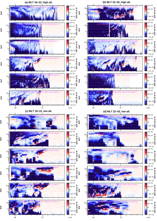
4.1 Basic properties of ion beamlets in PSBL and BPS Figure 1 shows examples of randomly chosen ion beamlet events as a function of energy and ILAT for different MLT, altitude and Kpconditions. In each subplot there are six
pan-els representing ion beamlets during varying Kpindex. The
six panels are ordered so that the Kpindex increases when
moving downward. The quantity shown is the S-variable (Eq. 1) in fixed linear scale. This is thus a new way to present ion data which is designed to reveal the ion beam-lets better than conventional plotting methods. In the top subplots we show examples of ion beamlets at R>4 RE (R
is the radial, i.e. geocentric distance) and in the bottom for
R<2.5RE. The left and right subplots are for 18–22 MLT
and 22–02 MLT, respectively.
For all plots it is seen that the first beamlet always appears at the boundary to the polar cap, i.e. in the PSBL. For cases where there are multiple beamlets, these occur in a broad latitudinal region adjacent to the polar cap, i.e. in the BPS re-gion. Usually the most poleward beamlet is the most intense, containing the highest energy fluxes.
It is seen in Fig. 1 that the Kpindex does not have a clear
effect on the beamlets.
The ion beamlets occurring at high altitudes generally have a steeper ILAT-energy slope compared to beamlets at low altitude.
The manual inspection also showed that the number of beamlets per auroral crossing is smaller at low altitude than at high altitude. Often at low altitude, only a single beamlet (VDIS) is seen at the PSBL. The effectively poorer spatial resolution at low altitude may explain the difference partly, but probably not fully. Quantitatively, the satellite footpoint moves 30–40 km during one 12 s TIMAS sampling period at low altitude while it moves less than 4 km per 12 s when
R>4 RE.
4.2 Statistics of ion beamlets in PSBL and BPS
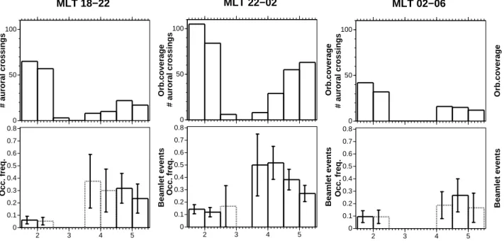
In Fig. 2 the occurrence frequency of ion beamlets as a func-tion of altitude for both high (>2) and low (≤2) Kp values
is shown. The three subplots correspond to different night-side MLT sectors. In the top panels of Fig. 2 the number of good auroral zone crossings containing a clearly identifi-able polar cap boundary in TIMAS data is shown for each radial distance bin. Notice that there is a gap in the middle radial distances (2.5−4RE) because TIMAS suffered a
high-voltage breakdown at the end of 1998 which resulted in a lack of sensitivity that would be very challenging to overcome in the present study. The bottom panels show the occurrence frequency of ion beamlets, i.e. the number of events contain-ing at least one beamlet divided by number of good auroral crossings. For all nightside MLT, the occurrence frequency of ion beamlets is highest around 4–5 RE. The occurrence
frequency for ion beamlets is highest for the midnight sec-tor (22–02 MLT). In this secsec-tor, the occurrence frequency at around 4–5 RE is 0.5. The occurrence frequency of ion
beamlets does not vary significantly with Kp.
5 Beamlet correlation with wave activity and electron anisotropy
The single ion beamlet in the PSBL is often the most intense, while the beamlets in the BPS are usually weaker. When looking at the corresponding distribution functions in veloc-ity space one finds that the most intense beamlets correspond to full ion shells, while the weaker beamlets appear as more or less plateaued distributions.
We look through all high-altitude (R>4 RE) events (36
to-tal) where TIMAS detects beamlets and the PWI instrument was operating (from 1 April 1996 to 16 September 1997). Six events were removed because they did not contain a clearly polar cap boundary probably due to extensive temporal vari-ations, leaving 30 events to study further.
The relevant frequency is the lower hybrid frequency. The considered 30 events span the radial distance range
R=4.8−5.4 REwhere the lower hybrid frequency varies
be-tween 100 and 170 Hz, assuming proton plasma with den-sity in the range 0.3–1 cm−3. In Table 1 we show the linear and rank correlation coefficient, averaged over the 30 events
2137:19970518 01:29−02:30 MLT=21.9, R=4.7, Kp=1 1 10 keV keV s3 m−6 −1e−13 −5e−14 0 5e−14 1e−13 2089:19970509 05:07−06:09 MLT=22, R=4.8, Kp=1.3 1 10 keV keV s3 m−6 −1e−13 −5e−14 0 5e−14 1e−13 289:19960531 01:37−02:48 MLT=21.2, R=5.3, Kp=1.7 1 10 keV keV s3 m−6 −1e−13 −5e−14 0 5e−14 1e−13 4020:19980518 21:48−22:36 MLT=22.1, R=4.2, Kp=2.7 1 10 keV keV s3 m−6 −1e−13 −5e−14 0 5e−14 1e−13 2257:19970609 04:03−05:05 MLT=19.8, R=4.8, Kp=5.7 1 10 keV keV s3 m−6 −1e−13 −5e−14 0 5e−14 1e−13 3942:19980502 12:50−13:51 MLT=21.8, R=4.8, Kp=6.7 65 70 ILAT 1 10 keV keV s3 m−6 −1e−13 −5e−14 0 5e−14 1e−13
(a) MLT 18−22, high alt.
2033:19970428 21:03−22:22 MLT=23.6, R=5.2, Kp=0.3 1 10 keV keV s3 m−6 −1e−13 −5e−14 0 5e−14 1e−13 3740:19980320 12:44−13:38 MLT=0.423, R=4.6, Kp=2 1 10 keV keV s3 m−6 −1e−13 −5e−14 0 5e−14 1e−13 3911:19980425 20:32−21:31 MLT=23.6, R=4.5, Kp=2.7 1 10 keV keV s3 m−6 −1e−13 −5e−14 0 5e−14 1e−13 3922:19980428 02:35−03:15 MLT=22.9, R=4, Kp=3 1 10 keV keV s3 m−6 −1e−13 −5e−14 0 5e−14 1e−13 1993:19970421 12:09−13:14 MLT=22.8, R=5.3, Kp=4.7 1 10 keV keV s3 m−6 −1e−13 −5e−14 0 5e−14 1e−13 1937:19970411 05:08−06:10 MLT=24, R=4.8, Kp=6.7 65 70 ILAT 1 10 keV keV s3 m−6 −1e−13 −5e−14 0 5e−14 1e−13 (b) MLT 22−02, high alt. 2302:19970617 08:57−09:06 MLT=20.9, R=2, Kp=1 1 10 keV keV s3 m−6 −1e−13 −5e−14 0 5e−14 1e−13 3117:19971115 14:54−15:07 MLT=21.4, R=2.3, Kp=2 1 10 keV keV s3 m−6 −1e−13 −5e−14 0 5e−14 1e−13 3133:19971118 13:56−14:08 MLT=21.5, R=2.3, Kp=4 1 10 keV keV s3 m−6 −1e−13 −5e−14 0 5e−14 1e−13 2258:19970609 06:28−06:37 MLT=22.2, R=2, Kp=5 1 10 keV keV s3 m−6 −1e−13 −5e−14 0 5e−14 1e−13 4838:19981114 03:53−04:04 MLT=22, R=2.1, Kp=5.7 1 10 keV keV s3 m−6 −1e−13 −5e−14 0 5e−14 1e−13 3155:19971123 00:14−00:23 MLT=20.3, R=2, Kp=7.3 65 70 ILAT 1 10 keV keV s3 m−6 −1e−13 −5e−14 0 5e−14 1e−13 (c) MLT 18−22, low alt. 275:19960528 06:02−06:13 MLT=23.2, R=2, Kp=1.3 1 10 keV keV s3 m−6 −1e−13 −5e−14 0 5e−14 1e−13 290:19960531 04:18−04:28 MLT=22.7, R=2, Kp=1.7 1 10 keV keV s3 m−6 −1e−13 −5e−14 0 5e−14 1e−13 822:19960915 00:20−00:29 MLT=1.41, R=1.9, Kp=2 1 10 keV keV s3 m−6 −1e−13 −5e−14 0 5e−14 1e−13 1702:19970227 00:14−00:24 MLT=1.82, R=2.1, Kp=3.3 1 10 keV keV s3 m−6 −1e−13 −5e−14 0 5e−14 1e−13 4809:19981107 11:18−11:36 MLT=22.9, R=2.5, Kp=4 1 10 keV keV s3 m−6 −1e−13 −5e−14 0 5e−14 1e−13 859:19960922 07:54−08:01 MLT=2.06, R=1.9, Kp=5.3 65 70 ILAT 1 10 keV keV s3 m−6 −1e−13 −5e−14 0 5e−14 1e−13 (d) MLT 22−02, low alt.
Fig. 1. Examples of multiple ion beamlets by Polar/Timas as a function of energy and ILAT for varying altitude, Kpand MLT conditions. The quantity shown is S(E), Eq. 1, in linear scale. Each subplot shows six panels with ion beamlets occurring during varying Kpindex, with increasing Kpvalues from top to bottom panel. Top plots show ion beamlets for radial distances >4 RE, and bottom plots for altitudes
≤2.5 RE. Left subplots show the ion beamlets for 18–22 MLT and right subplot for 22–02 MLT. Subplot a) thus shows examples of ion beamlets for 18–22 MLT at high altitudes, and subplot b) shows ion beamlets for high altitude but 22–02 MLT. The bottom subplots c) give example for ion beamlets at low altitudes for 18–22 MLT and d) for low altitudes and 22–02 MLT.
P. Janhunen et al.: Latitude-energy structure of multiple ion beamlets 871 0 50 100 # auroral crossings Orb.coverage 2 3 4 5 0 0.1 0.2 0.3 0.4 0.5 0.6 0.7 0.8 Occ. freq. Beamlet events MLT 18−22 0 50 100 # auroral crossings Orb.coverage 2 3 4 5 0 0.1 0.2 0.3 0.4 0.5 0.6 0.7 0.8 Occ. freq. Beamlet events MLT 22−02 0 50 100 # auroral crossings Orb.coverage 2 3 4 5 0 0.1 0.2 0.3 0.4 0.5 0.6 0.7 0.8 Occ. freq. Beamlet events MLT 02−06
Fig. 2. Top panels in each subplot show the orbital coverage of the Polar satellite, i.e. the number of good auroral crossings where “good” means that a clear polar cap boundary was seen in TIMAS data. Second panels show the occurrence frequency of ion beamlets by as a function of altitude, for Kp≤2 (filled dots) and for Kp>2 (triangles). Each subplot shows the occurrence frequency for 18–22, 22–02 and 02–06 MLT respectively.
studied, of nine (3×3) variable pairs. The correlated variable pair is of the form (E, P ) where E is one of three energy density quantities (free energy density, original free energy density and their difference, see section 3.3) and P is the PWI wave amplitude in one of three frequency ranges (26– 50 Hz, 50–300 Hz and 300–1000 Hz). The PWI original time resolution is 33 s, but was interpolated to 12 s before correlat-ing with TIMAS energy density quantities. The two lowest frequency ranges display almost equally good correlations. The difference of the original and the free energy density is best correlated with the waves, the original energy density it-self being nearly as good. Based on Table 1 and some more trials not reported here in detail we use the frequency range 26–500 Hz in what follows and use the original minus free energy as the ion beamlet measure.
Thus, from Table 1, the correlation between waves and ion beamlets is ∼50%. It can be asked whether this is high enough to be significant. There are at least three reasons why the correlation cannot be perfect. Firstly, the quantities often show variations in the same time scale as the time resolu-tion of the instruments, thus more correlaresolu-tion might be re-vealed if the time resolution was higher. Secondly, in many events TIMAS actually measures only every other 12-s inter-val which effectively halves the time reseolution. The gaps are filled by linear interpolation. Thirdly, our algorithm for finding the free and original energy finds at most one shell or plateau distribution in a given distribution. In cases where more than one shell or plateau exists simultaneously, only one of them is taken into account. We see from e.g. Fig. 1 that cases where multiple beamlets overlap are not rare.
Table 1. Average linear and rank correlation coefficient in the 30 events studied with free and original energy density and their differ-ence as well as PWI wave amplitude in three frequency ranges
26–50 50–300 300–1000 Hz Hz Hz FreeE lincorr 0.402 0.497 0.310 FreeE rankcorr 0.311 0.376 0.363 OrigE lincorr 0.458 0.523 0.331 OrigE rankcorr 0.479 0.500 0.480 OrigE-FreeE lincorr 0.452 0.490 0.324 OrigE-FreeE rankcorr 0.526 0.520 0.492
We now study how the beamlets correlate with wave ac-tivity by using two events considered in detail.
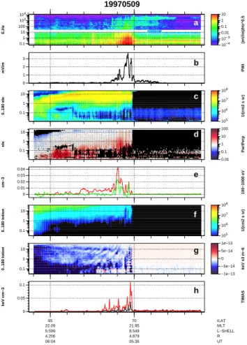
In Fig. 3 we show Polar data from various instruments for 9 May 1997. Panel (a) is the electric wave amplitude spectrogram combined from EFI (frequencies below 20 Hz) and PWI (frequencies above 26 Hz) data and panel (b) shows the PWI electric amplitude integrated between 26 Hz and 500 Hz interpolated to 12 s time resolution (originally 33 s). Panel (c) is the standard HYDRA electron differential en-ergy flux spectrogram and panel (d) is derived from that, showing the energy-dependent anisotropy (Sect. 3.2). The energy-dependent anisotropy is the ratio of the parallel ver-sus perpendicular distribution function, positive values (red) meaning Tk>T⊥type electron anisotropies. The red line in
0.1 1 10 100 103 104 E,Hz (mV/m)/Hz^0.5 10−4 10−3 0.01 0.1 1 10 0 1 2 3 mV/m PWI 0.1 1 10 0..180 ele 1/(cm2 s sr) 105 106 107 108 0.1 1 10 ele Par/Perp 0.01 0.1 1 10 100 0 0.01 0.02 0.03 0.04 cm−3 100−1000 eV 0.1 1 10 0..180 totion 1/(cm2 s sr) 105 106 107 108 0.1 1 10 0..180 totion keV s3 m−6 −1e−13 −5e−14 0 5e−14 1e−13 65 70 ILAT 0 0.05 0.1 keV cm−3 TIMAS 22.09 21.95 MLT 5.599 8.549 L−SHELL 4.206 4.879 R 06:04 05:36 UT 19970509 a b c d e f g h
Fig. 3. Polar data for event 9 May 1997: (a) EFI (<20 Hz) and PWI (>26 Hz) omnidirectional electric wave field amplitude spec-trograms between 0.1 Hz and 10 kHz, (b) PWI electric wave ampli-tude in frequency range 26–500 Hz, (c) HYDRA pitch-angle aver-aged electron differential energy flux spectrogram, (d) ratio of par-allel to perpendicular distribution function (Janhunen et al., 2004a),
(e) parallel versus perpendicular middle-energy anisotropy (0.1–1 keV) in red and up minus down anisotropy in green, (f) TIMAS pitch-angle averaged total ion differential energy flux spectrogram,
(g) quantity S (Eq. 1) computed from panel f, (h) “free” energy density of ion shell distributions in black, ’original’ minus “free” in red. The CPS/BPS boundary in this event is probably near ILAT 64. Panels b, e and h are correlated.
in the middle energy range (0.1−1 keV), computed as ex-plained in Sect. 3.2, while the green line is the up minus down anisotropy. Panel (f) is a standard TIMAS total ion dif-ferential energy flux spectrogram and panel (g) is the quan-tity S(E) derived from it using Eq. (1). Finally, panel (h) shows the “free” energy density of the ion shell distributions in black and the “original” minus “free” energy density in red, see Sect. 3.3 and Olsson et al. (2004).
Concerning the question what frequency waves correlate best with either of the quantity shown in panel (h), we found that in our events, the best correlation is usually provided by waves with frequency of the order of 100 Hz, e.g. 50–300 Hz. The correlation remains about equally good if the frequency range is extended to 26–500 Hz as we do in panel (b), see
also the discussion of Table 1 above. Above 500 Hz the correlation is sometimes reduced by auroral hiss emissions that are also visible in Fig. 3, e.g. above 70 ILAT they are the predominant emission that occurs most intensely above 1 kHz. In the data we are using here, the frequency range 10– 26 Hz is typically not covered, although in the event shown in Fig. 3, EFI does measure up to 20 Hz (40 samples per second) for a brief time near 71 ILAT. The correlation of 1–10 Hz waves between quantities in panel (h) is clearly inferior to 26–500 Hz, although not poor.
Figure 4 shows a second example event. Again the corre-lation between panels (b), (e) and (h) is good. Ion beamlets in the BPS and PSBL giving rise to noticeable shell distribu-tion free and original energy occur in the ILAT range 71–74. The correlation of the red line in panel (h) with the PWI wave amplitude in panel (b) is quite good in the sense that almost every peak is correlated, although the amplitude of the peaks does not always scale in the same way. We make the inter-pretation that the ion beamlets contain the free energy which is feeding the waves. A more detailed look of the PWI spec-trogram (not shown) indicates that the most important waves have frequency around 100 Hz, which is somewhat below the lower hybrid frequency and in good agreement with the sim-ulation results of Janhunen et al. (2003a). In that simsim-ulation, it was shown that ion Bernstein waves excited over very sim-ilar frequency range as seen in panel (a) can use an ion shell distribution free energy and grow to rather large amplitude and also energise electrons in the parallel direction. It is pos-sible that this process is in action in Fig. 4: there is good cor-relation between ion shell distributions and ∼100 Hz waves and, furthermore, the electron anisotropy (panel e, red line) also is enhanced at each wave amplitude peak of panel (b). Significant electron anisotropies also occur at 69–71 ILAT, i.e. outside the region of waves and ion shells. Perhaps this is explained by a finite lifetime of the electron anisotropies and continuous convection of the plasma towards lower ILAT.
In this paper we are only interested in ion beamlets and shell distributions occurring in the BPS and PSBL. We have marked the estimated CPS/BPS boundary in Fig. 4. The shell distribution free and original energy (panel h) are enhanced also at 65–66 ILAT, i.e. in the CPS, but this phenomenon is outside the scope of this paper.
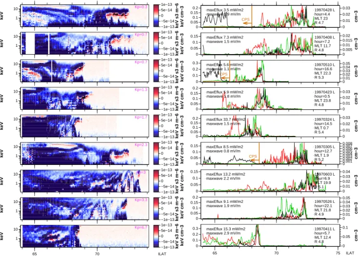
In Fig. 5 we show examples of events with ion beamlets, waves and electron anisotropies. The left-hand panel shows
S(E)(Eq. 1) for each event and the right-hand panel shows multiple lineplotted quantities for the corresponding event. The black line is the “original” minus “free” energy density associated with the ion shell distributions (same as red line in panels h earlier in Figs. 3 and 4). The red line is the elec-tron anisotropy (same as red line in panels e earlier) and the green line is the 26–500 Hz PWI amplitude (same as panel b earlier). The black line scale (keV cm−3) is on the left-hand vertical axis and the red line scale (cm−3) is on the right-hand axis. The scale of the green line (PWI amplitude) can be in-ferred from the maximum amplitude value (mV/m) shown textually on the left side of each panel. The maximum in-tegrated downward ion energy flux is also shown textually
P. Janhunen et al.: Latitude-energy structure of multiple ion beamlets 873 0.1 1 10 100 103 104 E,Hz (mV/m)/Hz^0.5 10−4 10−3 0.01 0.1 1 10 0 0.5 1 mV/m PWI 0.1 1 10 0..180 ele 1/(cm2 s sr) 105 106 107 108 0.1 1 10 ele Par/Perp 0.01 0.1 1 10 100 −0.005 0 0.005 0.01 0.015 cm−3 100−1000 eV 0.1 1 10 0..180 totion 1/(cm2 s sr) 105 106 107 108 0.1 1 10 0..180 totion keV s3 m−6 −1e−13 −5e−14 0 5e−14 1e−13 65 70 ILAT 0 0.05 0.1 0.15 0.2 keV cm−3 TIMAS 1.866 1.706 MLT 5.599 8.549 L−SHELL 4.31 5.023 R 10:16 09:46 UT 19970311 a b c d e f g h CPS −1.0×10⁶ 0.0×100 1.0×10⁶ 1.8×10⁶ −1.8×10 −1.0×106 0.0×100 1.0×10⁶ 1.8×10⁶ vPerp (m/s) vPar (m/s) 100 400 700 1e+03 4e+03 7e+03 1e+04 4e+04 7e+04 1e+05 4e+05 7e+05 1e+06 4e+06 7e+06 1e+07 4e+07 7e+07 1e+08 −1.0×10⁶ 0.0×100 1.0×10⁶ 1.8×10⁶ −1.8×10⁶ −1.0×10⁶ 0.0×100 1.0×10⁶ 1.8×10⁶ TOTION 19970311, 09:24:39 .. 09:24:51 vPerp (m/s) vPar (m/s)
Relative original energy 0.074884
100 400 700 1e+03 4e+03 7e+03 1e+04 4e+04 7e+04 1e+05 4e+05 7e+05 1e+06 4e+06 7e+06 1e+07 4e+07 7e+07 1e+08 −1.0×10⁶ 0.0×100 1.0×10⁶ 1.8×10⁶ −1.8×10⁶ −1.0×10⁶ 0.0×100 1.0×10⁶ 1.8×10⁶ TOTION 19970311, 09:27:34 .. 09:27:46 vPerp (m/s) vPar (m/s)
Relative original energy 0.0727459
100 400 700 1e+03 4e+03 7e+03 1e+04 4e+04 7e+04 1e+05 4e+05 7e+05 1e+06 4e+06 7e+06 1e+07 4e+07 7e+07 1e+08 −1.0×10⁶ 0.0×100 1.0×10⁶ 1.8×10⁶ −1.8×10 −1.0×106 0.0×100 1.0×10⁶ 1.8×10⁶ vPerp (m/s) vPar (m/s) 100 400 700 1e+03 4e+03 7e+03 1e+04 4e+04 7e+04 1e+05 4e+05 7e+05 1e+06 4e+06 7e+06 1e+07 4e+07 7e+07 1e+08 −1.0×10⁶ 0.0×100 1.0×10⁶ 1.8×10⁶ −1.8×10⁶ −1.0×10⁶ 0.0×100 1.0×10⁶ 1.8×10⁶ TOTION 19970311, 09:24:39 .. 09:24:51 vPerp (m/s) vPar (m/s)
Relative original energy 0.074884
100 400 700 1e+03 4e+03 7e+03 1e+04 4e+04 7e+04 1e+05 4e+05 7e+05 1e+06 4e+06 7e+06 1e+07 4e+07 7e+07 1e+08 −1.0×10⁶ 0.0×100 1.0×10⁶ 1.8×10⁶ −1.8×10⁶ −1.0×10⁶ 0.0×100 1.0×10⁶ 1.8×10⁶ TOTION 19970311, 09:27:34 .. 09:27:46 vPerp (m/s) vPar (m/s)
Relative original energy 0.0727459
100 400 700 1e+03 4e+03 7e+03 1e+04 4e+04 7e+04 1e+05 4e+05 7e+05 1e+06 4e+06 7e+06 1e+07 4e+07 7e+07 1e+08
Fig. 4. Polar data for event 11 March 1997. Format is similar to Fig. 3. The estimated CPS/BPS boundary is also shown. On the bottom of the main plot, three example distribution functions corresponding to shell distributions are shown as well.
in mW/m2. On the right we show the event date, the let-ter “L” or “R” indicating whether Polar moves to the left (L) or to the right (R) in the plot, an approximate central UT hour of the event and the mean MLT and radial distance
Rvalue during the event. An estimated CPS/BPS boundary position is marked where applicable. Finally, the Kp value
for each event is shown on the left-hand panel near the up-per right corner. In Fig. 5 the events are arranged so that
Kp increases from top to bottom. The events were selected
among cases where energy-dispersed structures (left panel)
are clearly seen and which represent many different Kp
con-ditions. During selection process, no attention was paid to how well the variables in the right panel correlate among themselves.
We shall not discuss each event in Fig. 5 in detail. We point out that the correlation between the 26–500 Hz waves and the shell distribution original minus free energy density is rather good (∼50%) in all cases, although not all peaks seen in wave data can be identified in ion data and vice versa.
Kp=0.3 1 10 keV keV s3 m−6 −1e−13 −5e−14 0 5e−14 1e−13 Kp=0.7 1 10 keV keV s3 m−6 −1e−13 −5e−14 0 5e−14 1e−13 Kp=0.7 1 10 keV keV s3 m−6 −1e−13 −5e−14 0 5e−14 1e−13 Kp=1.3 1 10 keV keV s3 m−6 −1e−13 −5e−14 0 5e−14 1e−13 Kp=1.7 1 10 keV keV s3 m−6 −1e−13 −5e−14 0 5e−14 1e−13 Kp=2.3 1 10 keV keV s3 m−6 −1e−13 −5e−14 0 5e−14 1e−13 Kp=3 1 10 keV keV s3 m−6 −1e−13 −5e−14 0 5e−14 1e−13 Kp=3.3 1 10 keV keV s3 m−6 −1e−13 −5e−14 0 5e−14 1e−13 Kp=6.7 65 70 ILAT 1 10 keV keV s3 m−6 −1e−13 −5e−14 0 5e−14 1e−13 CPS 19970428 L hour=4.4 MLT 23 R 4.7 maxEflux 3.5 mW/m2 maxwave 1.9 mV/m 0 0.05 0.1 0.15 0.2 0 0.01 0.02 0.03 keV cm−3 cm−3 19970408 L hour=7.2 MLT 11.7 R 4.8 maxEflux 7.3 mW/m2 maxwave 1.5 mV/m 0 0.05 0.1 0.15 0 0.005 0.01 0.015 0.02 keV cm−3 cm−3 CPS 19970510 L hour=16.6 MLT 22.3 R 5.3 maxEflux 5.6 mW/m2 maxwave 1.1 mV/m 0 0.1 0.2 0.3 0 0.01 0.02 0.03 0.04 0.05 keV cm−3 cm−3 19970423 L hour=0.5 MLT 23.8 R 4.8 maxEflux 5.9 mW/m2 maxwave 1.8 mV/m 0 0.05 0.1 0.15 0.2 0 0.01 0.02 0.03 keV cm−3 cm−3 19970324 L hour=14.5 MLT 0.7 R 5.4 maxEflux 33.7 mW/m2 maxwave 1.5 mV/m 0 0.05 0.1 0.15 0.2 0 0.01 0.02 0.03 keV cm−3 cm−3 CPS 19970305 L hour=12.7 MLT 1.9 R 5.2 maxEflux 8.5 mW/m2 maxwave 0.8 mV/m 0 0.05 0.1 0.15 0 0.001 0.002 0.003 0.004 0.005 0.006 0.007 0.008 keV cm−3 cm−3 19970603 L hour=6.9 MLT 19.9 R 5.1 maxEflux 13.2 mW/m2 maxwave 2.2 mV/m 0 0.05 0.1 0.15 0 0.01 0.02 0.03 0.04 keV cm−3 cm−3 19970526 L hour=22.1 MLT 21.8 R 4.9 maxEflux 9.1 mW/m2 maxwave 1.9 mV/m 0 0.05 0.1 0.15 0.2 0 0.01 0.02 0.03 0.04 0.05 keV cm−3 cm−3 19970411 L hour=5.7 MLT 12.4 R 4.8 maxEflux 15.3 mW/m2 maxwave 2.9 mV/m 65 70 75 ILAT 0 0.1 0.2 0.3 0 0.05 0.1 keV cm−3 cm−3
Fig. 5. Each panel is one event, where the Polar/Timas satellite passes through the auroral zone. Black line is free energy from TIMAS (scale on the left) and red line is magnitude of electron anisotropy from HYDRA (scale on the right). Green line is unnormalised perpendicular wave power from EFI (12-s averaged); its attained maximum is written on the left (“maxwave”). Maximum downward ion energy flux from TIMAS during time when free energy exceeds 0.02 keV cm−3is also given; the value is given at the ionospheric level by multiplying the measured value by flux tube scaling factor. Event date and average UT-hour, MLT and radial distance are also given. The letter L(R) after the date indicates that satellite is moving to the left (right), i.e. towards decreasing (increasing) ILAT.
6 Summary and discussion
The motivation for this study is to show observations of mul-tiple ion beamlets in the PSBL and BPS regions. Multi-ple beamlets have previously been predicted in theoretical work. We present the basic properties of multiple ion beam-lets in the PSBL and BPS and study how the beambeam-lets sta-tistically depend on altitude, MLT and Kp. For 30 events
we had the possibility to study high frequency wave data (Polar/PWI), electron anisotropy (Polar/HYDRA) and free energy of ion shells in ion beamlets (Polar/TIMAS). In all events we found that the parameters correlated and in the study we present some examples of individual events. We believe that the multiple ion beamlets, waves (26–500 Hz) and electron anisotropy are all important parameters in the auroral process and are part of the energy chain in the upper part of the auroral acceleration region. The frequency inter-val can be made more narrow than 26–500 Hz without much
reducing the correlation as long as the range 50–180 Hz or so is included. Below we summarize our findings.
1. Ion beamlets occur in the PSBL and BPS. They are most common in the midnight and late evening MLT sectors. 2. The ion beamlets are about equally common at low (R<3 RE) and high (R>4 RE) altitude, but their types
are different. The low-altitude events usually contain only one energy-latitude dispersed feature (VDIS) of-ten over broad ILAT range, while multiple beamlets are often observed at high altitude. The high altitude beam-lets usually show a steeper energy-latitude profile than the low altitude ones.
3. Ion beamlets probably occur on most auroral crossings in the nightside and late evening MLT sectors where the observation is not too much disturbed by a motion of the plasma sheet while Polar is crossing it. Based on the
P. Janhunen et al.: Latitude-energy structure of multiple ion beamlets 875 manual search the occurrence frequency in the evening
and midnight MLT sectors is 30–50%.
4. The occurrence frequency and other characteristics of the beamlets do not markedly depend on the Kpindex.
5. The ion beamlets often correlate with electron anisotropy (0.1–1 keV electrons) and electrostatic waves (26–500 Hz).
The study of ion beamlets is related to the question of what powers stable discrete auroral arcs and gives the highly struc-tured latitudinal profiles of the low-altitude electron energy flux. The ion beamlet study emphasises the morphology in latitude-energy space whereas our earlier study of the free energy density of ion shell distributions (Olsson et al., 2004) emphasised the more quantitative energy aspect. One moti-vation for this morphological study is that the 6-D ion phase space could possibly contain free energy in subtler ways than in the form of traditional ion shell distributions (e.g. for lower hybrid drift waves, spatial inhomogeneities could be impor-tant). Thus the ion shell and beamlet approaches are comple-mentary: the ion shell approach is quantitative, but more lim-ited in the type of structures that are considered, the beamlet approach is qualitative and morphological, but reveals more general structures.
A natural question first hinted at by Ashour-Abdalla et al. (1992) is: are ion beamlets responsible for the observed rich latitudinal structure of auroral arcs and arc systems? Al-though we cannot give a definite answer yet, based on the data presented here we consider this as a real possibility. The latitudinal scale sizes and extents of the beamlets correspond to that of typical arc structures. It takes Polar about half an hour to pass through the beamlet region above R=4 RE;
al-ready the fact that beamlets are consistently observed is by itself an indication that they have something to do with per-sistent, slowly varying structures such as stable auroral arcs. In disturbed events the energy-latitude structures break up, which is also what happens to auroral arcs in such condi-tions.
If the ion beamlets are responsible for creating stable dis-crete auroral arcs, the overall energetics should also find an explanation. The net parallel downward ion energy flux is of-ten sufficient locally to power the aurora below, but there are usually nearby regions where the net ion energy flux is up-ward (often this is due to intense upgoing ion beams). Thus, energetically the parallel downward ion energy flux does not seem to be quite sufficient to power stable aurora plus ion beams. One must remember, however, that the plasma sheet ions can also move considerably in the perpendicular direc-tion during one bounce period. While drifting earthward and westward, they are also continually energised by the betatron and Fermi acceleration (i.e. they gain energy from the large-scale electric field). A study of the auroral energy balance taking into account also the perpendicular components of the energy flux vector should therefore be made before the en-ergetic importance of plasma sheet ions in powering stable aurora can be answered.
Finally, we comment item 2 listed above, i.e. why at low altitude one rarely sees multiple beamlets, but usually one sees only one velocity-dispersed structure. The latitudinal width of the single structure is also typically larger than at high altitude, i.e. the slope of the energy versus latitude fea-ture is smaller. The fact that the instrument time resolution of 12 s is not enough at low altitude to resolve latitudinally nar-row structure is one factor, but we think that it is not enough to explain this finding. Sensitive and high time resolution ion instruments on satellites at low and middle altitude would be good for studying this question.
Acknowledgements. We are thankful to H. Laakso and F. S. Mozer
for EFI data, C. A. Kletzing and J. D. Scudder for providing HY-DRA data and J. S. Pickett, D. A. Gurnett for PWI data. The work of PJ was supported by the Academy of Finland and that of AO by the Swedish Research Council. WKP acknowledges support from NASA grant NAG5-11391.
The editor in chief thanks two referees for their help in evaluat-ing this paper.
References
Ashour-Abdalla, M., Zelenyi, L. M., Bosqued, J.-M., Peroomian, V., Wang, Z., Schriver, D., and Richard, R. L.: The formation of the wall region: consequences in the near Earth magnetotail, Geophys. Res. Lett., 19, 1739–1742, 1992.
Ashour-Abdalla, M., Berchem, J. P., B¨uchner, J., and Zelenyi, L. M.: Shaping of the magnetotail from the mantle: global and local structuring, J. Geophys. Res., 98, 5651–5676, 1993.
Ashour-Abdalla, M., Zelenyi, L. M., Peroomian, V., Richard, R. L., and Bosqued, J. M.: The mosaic structure of plasma bulk flows in the Earth’s magnetotail, J. Geophys. Res., 100, 19 191–19 209, 1995.
Baumjohann, W., Paschmann, G., and L¨uhr, H.: Characteristics of high-speed ion flows in the plasma sheet, J. Geophys. Res., 95, 3801–3809, 1990.
Bosqued, J. M., Ashour-Abdalla, M., El Alaoui, M., Zelenyi, L. M., and Berthelier, A.: AUREOL-3 observations of new boundaries in the auroral ion precipitation, Geophys. Res. Lett., 20, 1203– 1206, 1993a.
Bosqued, J. M., Ashour-Abdalla, M., El Alaoui, M., Peroomian, V., Zelenyi, L. M., and Escoubet, C. P.: Dispersed ion structures at the poleward edge of the auroral oval: Low-altitude observations and numerical modeling, J. Geophys. Res., 98, 19 181–19 204, 1993b.
Burkhart, G. R., Dusenbery, P. B., Speiser, T. W., and Lopez, R. E.: Hybrid simulations of thin current sheets, J. Geophys. Res., 98, 21 373–21 390, 1993.
Chen, J. and Palmadesso, P. J.: Chaos and nonlinear dynamics of single-particle orbits in a magnetotaillike magnetic field, J. Geo-phys. Res., 91, 1499–1508, 1986.
Delcourt, D. C. and Martin, R. F.: Pitch angle scattering near energy resonances in the geomagnetic tail, J. Geophys. Res., 104, 383– 394, 1999.
Dusenbery, P. B. and Lyons, L. R.: The generation of electrostatic noise in the plasma sheet boundary layer, J. Geophys. Res., 90, 10 935–10 943, 1985.
Eastman, T. E., Frank, L. A., Peterson, W. K., and Lennartsson, W.: The plasma sheet boundary layer, J. Geophys. Res., 89, 1553– 1572, 1984.
Elphic, R. C. and Gary, S. P.: ISEE observations of low frequency waves and ion distribution function evolution in the plasma sheet boundary layer, Geophys. Res. Lett., 17, 2023–2026, 1990. Grigorenko, E. E., Fedorov, A., and Zelenyi, L. M.: Statistical study
of transient plasma structures in magnetotail lobes and plasma sheet boundary layer: Interball-1 observations, Ann. Geophys., 20, 329–340, 2002,
SRef-ID: 1432-0576/ag/2002-20-329.
Grigorenko, E. E., Fedorov, A., Zelenyi, L. M., and Sauvaud J.-A.: Coupling of transient plasma structures observed in the plasma sheet boundary layer and in the auroral region, Adv. Space Res., 31, 5, 1271–1276, 2003.
Gurnett, D. A., Persoon, A. M., and Randall, R. F. et al.: The Polar Plasma Wave Instrument, Space Sci. Rev., edited by Russell, C. T., Kluwer Acad., 71, 597–622, 1995.
Harvey, P., Mozer, F. S., Pankow, D., Wygant, J., Maynard, N. C., Singer, H., Sullivan, W., Anderson, P. B., Pfaff, R. Aggson, T., Pedersen, A., Falthammar, C. G., and Tanskanen, P.: The electric field instrument on the polar satellite, Space Science Reviews 71, 583–596, 1995.
Hirahara, M., Mukai, T., Nagai, T., Kaya, N., Hayakawa, H., and Fukunishi, H.: Two types of ion energy dispersions observed in the nightside auroral regions during geomagnetically disturbed periods, J. Geophys. Res., 101, 7749–7767, 1996.
Hirahara, M., Mukai, T., Sagawa, E., Kaya, N., and Hayakawa, H.: Multiple energy-dispersed ion precipitations in the low-latitude auroral oval: evidence of E×B drift effect and upward flowing ion contribution, J. Geophys. Res., 102, 2513–2530, 1997. Janhunen, P., Olsson, A., Vaivads, A., and Peterson, W. K.:
Gener-ation of Bernstein waves by ion shell distributions in the auroral region, Ann. Geophys., 21, 1–11, 2003a.
Janhunen, P., Olsson, A., Laakso, H., and Vaivads, A.: Middle-energy electron anisotropies in the auroral region, Ann. Geo-phys., 22, 1–13, 2004a.
Janhunen, P., Olsson, A., and Laakso, H.: The occurrence frequency of auroral potential structures and electric fields as a function of altitude using Polar/EFI data, Ann. Geophys., 22, 1233–1250, 2004b.
Lennartsson, O. W., Trattner, K. J., Collin, H. L., and Peterson, W. K.: Polar/TIMAS survey of earthward field-aligned proton flows from the near-midnight tail, J. Geophys. Res., 106, 5859–5872, 2001.
Olsson, A., Janhunen, P., Peterson, W. K., and Laakso, H.: Ion shell distributions as free energy source for plasma waves on auroral field lines mapping to plasma sheet boundary layer, Ann. Geo-phys., 22, 2115–2133, 2004,
SRef-ID: 1432-0576/ag/2004-22-2115.
Olsson, A. and Janhunen, P.: Some recent developments in un-derstanding auroral electron acceleration processes, IEEE Trans. Plasma Sci., 31, 1178–1191, 2003.
Onsager, T. G. and Mukai, T.: Low altitude signature of the plasma sheet boundary layer: Observations and model, Geophys. Res. Lett., 22, 855–858, 1995.
Sauvaud, J.-A., Popescu, D., Delcourt, D. C., Parks, G. K., Brit-tnacher, M., Sergeev, V., Kovrazhkin, R. A., Mukai, T., and Kokubun, S.: Sporadic plasma sheet ion injections into the high-altitude auroral bulge: satellite observations, J. Geophys. Res., 104 28 565–28 586, 1999.
Schriver, D. and Ashour-Abdalla, M.: Generation of high-frequency broadband electrostatic noise: the role of cold elec-trons, J. Geophys. Res., 92, 5807–5819, 1987.
Scudder, J. D., Hunsacker, F., and Miller, G. et al.: Hydra − A 3-dimensional electron and ion hot plasma instrument for the Polar spacecraft of the GGS mission, Space Sci. Rev., 71, 459–495, 1995.
Shelley, E. G., Ghielmetti, A. G., Balsiger, H., Black, R. K., Bowles, J. A., Bowman, R. P., Bratschi, O., Burch, J. L., Carl-son, C. W., Coker, A. J., Drake, J. F., Fischer, J., Geiss, J., John-stone, A., Kloza, D. L., Lennartsson, O. W., Magoncelli, A. L., Paschmann, G., Peterson, W. K., Rosenbauer, H., Sanders, T. C., Steinacher, M., Walton, D. M., Whalen B. A., and Young, D. T.: The Toroidal Imaging Mass-Angle Spectrograph (TIMAS) for the Polar Mission, Space Science Rev., 71, 1–4, 1995.
Winningham, D., Yasuhara, F., Akasofu, S.-I., and Heikkila, W. J.: The latitudinal morphology of 10-eV to 10-keV electron fluxes during magnetically quiet and disturbed times in the 21:00– 03:00 MLT sector, J. Geophys. Res., 80, 3148–3171, 1975. Zelenyi, L. M., Kovrazkhin, R. A., and Bosqued, J. M.:
Velocity-dispersed ion beams in the nightside auroral zone: AUREOL 3 observations, J. Geophys. Res., 95, 12 119–12 139, 1990.