Dynamics of belt-driven servomechanisms : theory and experiments

(1)

Dynamics of Belt-Driven Servomechanisms

Theory and Experiments

by

Dhanushkodi D. Mariappan

Bachelor of Technology (B.Tech), Mechanical Engineering

Indian Institute of Technology, Madras 2001

Submitted to the Department of Mechanical Engineering

in partial fulfillment of the requirements for the degree of

Master of Science in Mechanical Engineering

at the

MASSACHUSETTS INSTITUTE OF TECHNOLOGY

June 2003

@

Massachusetts Institute of Technology 2003. All rights reserved.

Author ...

...

Department of Mechanical Engineering

May 23, 2003

Certified by...

...

Samir A. Nayfeh

Assistant Professor

sis Supervisor

Accepted by ...

...

Ain A. Sonin

Chairman, Department Committee on Graduate Students

MASSACHUSETTS INSTITUTE OF TECHNOLOGY

JUL 0 8 2003

(2)

t

I

/

K.

i')

7 4

a

(3)

Dynamics of Belt-Driven Servomechanisms

Theory and Experiments

by

Dhanushkodi D. Mariappan

Submitted to the Department of Mechanical Engineering on May 23, 2003, in partial fulfillment of the

requirements for the degree of

Master of Science in Mechanical Engineering

Abstract

There is an ever increasing demand for high speed precision positioning systems from a wide range of industries. These machines typically employ ball-screws, linear motors, or belt-drives and operate in closed loop to achieve high performance. In this thesis, we study the dynamics of belt-driven servomechanisms. In these belt-driven machines,

the primary limitation to the performance arises from the belt compliance. The

performance is characterized by parameters which include bandwidth, tracking in the presence of disturbances, etc. We model the axial dynamics of the belt drives and discuss collocated and noncollocated feedback strategies. The design and assembly of a belt-driven linear motion stage is explained in detail. We measure the transfer functions through sine sweep measurements to verify the theoretical model. Damping plays a key role in determining the maximum achievable bandwidth of the belt-driven servomechanism. We present a model for the microslip phenomenon and quantify the damping that arises out of microslip. In summary, this thesis lays out a dynamic model of belt-driven servos, a model for microslip, a detailed design process, and experimental methods for measuring transfer functions.

Thesis Supervisor: Samir A. Nayfeh Title: Assistant Professor

(4)

(5)

Acknowledgment

First of all, I would like to thank Prof. Samir Nayfeh for giving me the opportunity to work on this exciting project. He continues to amaze me with his vast treasure house of knowledge and remarkable physical intuition. His deep insights in design, dynamics, controls and his excellent analytical depth always sets standards I strive to achieve. He has been very tolerant in admitting all the costly mistakes I did in the course of completion of this work. I would like to thank Prof. Sanjay Sarma for his encouraging words and help in moments of trouble. Sanjay's energy is incredible and I cherish the moments I spent listening to his words of wisdom. My undergraduate advisor Prof. V. Ramamurti has been a great inspiration in my academic path during and after my days at IIT, Madras. I would like to thank Kripa for his invaluable guidance and support. In addition to his lessons on dynamics theory and experiments, he has been a great mentor . I owe a lot to Kripa for the time he has spent teaching me. Mauricio always answered my questions patiently and suggested references. I owe a significant percentage of my design knowledge to him. Justin Verdirame is a very resourceful person. I always admired his cool and composed approach and I learnt to talk things with high signal to noise ratio. I consider myself unfortunate not to have worked with Greg for he is such a vibrant man with lots of design expertise. Andrew Wilson, a cheerful companion has answered my questions for the nth time without complaining.

I also thank Nader and Lei for their help. I always worked with machines which

needed atleast two people to handle and I thank Justin, Mauricio, Jonathan, Sup and others in the lab who took time off from their work and helped me. The LMP machine shop experience was fun and a lot of learning. I would like to thank Mark and Jerry for all the hours they spent teaching me patiently and admitting my mistakes. I acknowledge Jonathan's help in the file conversion issues with Solidworks drawings. I would like to thank Rick for his help with LVDT and other lessons. Hari, Srini and Madhu have been excellent companions and motivators. I thank Srini, Ajay and Hari for patiently proof reading my thesis and giving critical comments. Ajay has been a great companion who always made me set high standards in research and work

(6)

towards achieving them. I also thank Anand anna, Carlos, Karen, Vijay, Sriram, Harsh, Mahadevan, Shorya, Rama, and many others who were directly or indirectly involved in succesful completion of this work. Above all, I thank my appa, amma, murugappa, aachi, Juno and Venkatesh who were with me and will continue to be with me when it matters most. God is great and He has helped me strive, seek, find and not to yield.

(7)

List of Figures

2-1 Two-degree-of-freedom model . . . . 21

2-2 Collocated transfer function . . . . 33

2-3 Noncollocated transfer function . . . . 34

2-4 The effect of change in stiffness in the noncollocated transfer function 35 2-5 The effect of damping in the noncollocated transfer function . . . . . 36

2-6 Three-degrees-of-freedom model . . . . 36

2-7 Closed-loop servomechanism . . . . 37

2-8 Transfer function _x . . ... .. ... 37

1 2-9 3 DOF model -collocated transfer function . . . . 38

2-10 3 DOF model -noncollocated transfer function . . . . 39

2-11 Nyquist representation of crossover frequencies, Varanasi [3] . . . . . 40

2-12 Adding phase at cross over 3 leading to instability, Varanasi [3] . . . 41

2-13 Nyquist interpretation of robust gain margin (RGM) and phase margin (PM ), Varanasi [3] . . . . 42

3-1 Two spheres in contact under normal and tangential load . . . . 47

3-2 A typical belt drive showing the control volumes on the driven and driving pulleys . . . . 52

3-3 Free body diagram to show the forces on the belt . . . . 53

3-4 Variation of loss factor with friction coefficient p for different values of drive ratio n . . . . 59

4-1 The m achine . . . . 79

(12)

4-3 Assembly procedure to align the drive mount on the base . . . . 81

4-4 Air bearing assembly . . . . 82

4-5 Measuring the flyheight . . . . 82

4-6 Assembling the belt between the blocks . . . . 83

4-7 Pre-tensioning mechanism . . . . 83

4-8 Stiffness of the 40 mm flat air bearings [22] . . . . 84

4-9 Stiffness of the 50 mm flat air bearings [22] . . . . 85

4-10 Figure showing the pitch, roll and yaw axes of the carriage . . . . 86

4-11 Load-deflection characteristics of ball bearings [24] (Reprinted with permission from the author) . . . . 86

4-12 Comparision of preloaded versus non preloaded bearings [24] (Reprinted with permission from the author) . . . . 87

4-13 Locknut and lockwasher mounted on a threaded shaft (Reprinted from Whittet Higgins catalog with permission) . . . . 87

4-14 Current mode operation . . . . 88

5-1 Sine sweep experimental setup -Schematic . . . . 90

5-2 Measured and predicted collocated transfer function . . . . 91

5-3 Measured and predicted noncollocated transfer function . . . . 92

A-i Equivalent circuit of a DC motor . . . . 97

A-2 Equivalent-circuit representation of commutation . . . . 99

A-3 Voltage mode operation . . . . 101

B-i Drawing of the pulley . . . . 104

B-2 Drawing of the carriage plate 1 . . . . 105

B-3 Drawing of the carriage plate 2 . . . . 106

B-6 Drawing of the motor mount - Front view . . . . 109

(13)

List of Tables

2.1 Belt parameters . . . .

2.2 Mode shape - eigenvectors . . . .

2.3 The rigid body modes . . . .

4.1 Specifications: BM500E . . . .

4.2 Coupling dimensions and specifications . . .

4.3 Bearing nomenclature 7909A5 . . . .

4.4 Loading conditions and fits [23] . . . .

A.1 Inner-rotor versus outer-rotor BLDC motors

A.2 PMDC Vs BLDC Motors . . . . . . . . 23 . . . . 26 . . . . 28 . . . . 63 . . . . 65 . . . . 69 . . . . 70 . . . . 99 . . . . 100

(14)

(15)

Chapter 1 Introduction

Precision positioning systems are essential in a wide range of industries. These in-clude the eiefniconductor,-machine tool, robotics, material handling, packaging, data storage, and printing industries. Typically these systems use rotary actuators, such as brushless DC motors and convert the rotary motion to linear motion using me-chanical power transmission elements like belts, chains, ball screws, or lead screws. In addition, linear motors are used in several applications. The choice of the drive system is often based on the following factors which might vary depending on the application 1. speed 2. positioning accuracy 3. repeatability 4. range of travel 5. load-carrying capacity

(16)

1.1 Servomechanisms: Feedback

-

Performance

Cri-teria

These precision machines may or may not operate in closed loop. When not operated in closed-loop, they run in open loop using actuators like stepper motors. Open-loop control is simpler to implement since there is no need for sensors. Feedback control is more complex and may cause stability problems, but one can achieve significant im-provements in the performance of these precision machines using closed-loop control. When compared to open-loop control, feedback can be used to

1. reduce steady-state error due to disturbances by a factor of 1 + L where L is

the loop gain. L is the product of the controller and plant transfer functions 2. reduce the system's transfer function sensitivity to parameter variations

3. speed up the transient response

4. reduce the sensitivity of the output signal to parameter changes

1.1.1 Parameters of Performance

The two most important issues that concern the designer while designing a machine that operates in closed loop are the stability and performance. The broad classifica-tions of stability fall into two categories

1. External (OR) Input-Output Stability

2. Asymptotic Stability (OR) Internal Stability

In most cases, these two notions of stability converge as we often work with SISO sytems that are completely observable and controllable. The most appropriate way of characterizing stability will be, in the open loop frequency response L(jw), the phase be greater than -1800 at the cross-over frequency.

Primarily, one has to make sure that the system (in our case, the machine) is stable under closed-loop control. Once we have a stable system, we can improve the

(17)

performance of the system by designing the machine and the controller to meet the following closed loop performance specifications.

1. Trajectory Tracking

2. Disturbance Rejection

3. Noise Rejection

4. Performance Robustness

For detailed descriptions of each of these performance specifications, refer to [1] and

[2]

1.1.2 Design for Closed-Loop Performance [3]

The closed-loop performance specifications that are mentioned in the previous section depend on the loop transmission L. The loop transmission encompasses the plant and the controller dynamics. Therefore, it is important that the controller and the plant be designed simultaneously to extract the best possible performance out of these precision machines. This approach to solving the inverse problem of motion control was addressed by Varanasi and Nayfeh [3]. The inverse problem in motion control can be stated as: 'Given the performance specifications, design the loop transmission.' In

[3], the authors demonstrate this inverse approach with a case study on a ball-screw

servo system. The ultimate goal in this approach is to be able to obtain closed-form expressions which serve as strict guidelines for a mechanical designer who sets out to solve a 'design of precision machines for performance' problem. In this thesis, we lay out the design of a belt-driven linear motion stage for dynamic performance.

1.1.3 Limitations

The solution to the inverse problem necessitates a good model of the dynamics of the system. In this thesis, we develop a model of the dynamics and study the maximum bandwidths attainable with collocated and noncollocated control. The bandwidth

(18)

of the belt-driven servomechanism is limited by the drive resonance that arises from the compliance of the belt. In addition, if the stiffness of the components in the structural loop are not high enough, the compliances add up in series and bring down the stiffness of the drive. This translates in the form of the axial resonant frequency of the drive. The lower the resonant frequency, the lower the attainable bandwidth and hence the larger the time constant of the machine. Hence serious consideration is to be given to the design of various joints, preloading of bearings, choice of the coupling, optimization of the structural loop. Damping of the resonant peak also plays a role in determining the bandwidth. The amount of damping determines the degree of robustness of the system. In a belt drive, the question of adding deterministic damping in the load path is yet an unsolved problem. In this thesis, we investigate the significance of the damping that arises out of microslip in belt drives. We discover that the damping that arises out of microslip is insignificant and hence one has to find ways to add damping into the system.

1.2 Contributions

1. A model of the dynamics of the belt-drive.

2. A model for microslip in belt-drives.

3. Development of a design for stiffness approach with details on component

se-lection and the assembly process.

4. Experimental validation of the theoretical results by transfer function measure-ments.

(19)

Chapter 2 Modeling the Axial Dynamics of

the Belt Drive

2.1 Introduction

The axial resonance that arises from the compliance of the belt limits the performance of the belt-driven servomechanism. In this chapter, we derive the equations of motion for the drive and obtain a closed-form expression for the axial resonance which de-pends on the inertias in motion: the drive pulley inertia (Ji), the idler pulley inertia

(J2) and the mass of the carriage (M). In the subsequent chapters on the design of

the belt drive, we lay emphasis on the importance of the various compliances in the dynamic loop. Our model treats the belt compliance as the dominant compliance. This will not hold true if a bad design of the various components of the machine leads to one or more compliances at parts of the machine other than belt like joints, couplings, and so on. The most important assumptions are:

1. The mass of the belt is very small compared with the rest of the inertia.

2. The idler pulley inertia is lumped on to the carriage inertia.

(20)

We can check the validity of these assumptions depending on how well the experi-mental results match with theoretical predictions.

2.2 Modeling the Dynamics

The distributed inertia of the belt is negligible compared to the rest of the inertia in the system. This allows development of a lumped parameter model consisting of discrete masses connected by springs and dampers. Thus, the problem formulation involves a set of ordinary differential equations, the solutions of which propagate in time; these are commonly referred to as the initial value problems. If the inertia of the belt were to be included, it becomes a continuous system. The motion of such continuous systems is described by variables depending not only on time but also on spatial position. These are governed by partial differential equations. For continuous systems, the equations of motion are derived by formulating the problem

using Lagrangian mechanics. Then it becomes a boundary value problem where

solutions satisfy a differential equation in a given open domain and certain conditions on the boundaries of the system. A very detailed description of distributed parameter systems is available in [4]. In addition, the interested reader can refer to [1] and [5] for an introduction to modeling of dynamical systems and their control.

2.2.1 Model for the Belt Drive

The torque developed by the motor provides the actuation for the system. We

rep-resent this torque by T. J is the overall inertia on the drive side which comprises of

the inertia of the motor and the drive pulley inertia. We can lump these two inertias together if the torsional stiffness of the coupling that connects the motor shaft to the pulley shaft is very high. We will lay more emphasis on this fact in the Chapter 4. In

the Fig. 2-1, F refers to the generalized force which is the torque T. The coordinates

X1 and X2 represent the displacements of the drive pulley and the carriage

respec-tively. X1 and X2 will be referred to as 0 and x2 through the rest of this chapter. The

(21)

X, X2

F M1 2 n

K3

Figure 2-1: Two-degree-of-freedom model

r is the radius of the pulley. Since the pulley m3 is an idler, it does not transmit

any torque. Provided that the inertia M3 is small, the tensions on either side of the

pulley are equal. Hence, we can consider springs K2 and K3 to be in series. Their

equivalent stiffness is given by K' = K2K. Hence, the system reduces to a two-mass

system held together by two springs K1 and K' in parallel.

Writing the equations of motion for this system, we obtain

JiO + K(rO - X2) = 7 (2.1)

(M3 + m2)f 2 + K(x2 - rO) = 0 (2.2)

Here, K represents the overall stiffness. K1 is the stiffness of the steel belt between

the drive pulley and the carriage given by 1, where 1 is the length of the belt

between the carriage and the drive pulley. From these equations of motion, we derive expressions for the transfer functions by taking Laplace transforms, in order to obtain the behaviour of the system in the frequency domain. This leads to the following set of equations.

J1s2E + K(rG - X2)r = r (2.3)

(M2 + m3)s2X2 + K(X2 - r3) = 0 (2.4)

Here, X2 and

E

are functions of s. Solving these equations, we obtain the collocated

(22)

(s) I(S2 + )

- 2 +M3(2.5)J,

T(s) s2(S2 + K(m + ())

X2(s) Kr 1

T(s) Ji(m₂+ M3) s2(M2 + K(4 + ₍₂₎₎

The collocated and noncollocated transfer functions are so named because of the location of the sensors with respect to the actuator. In the former, a rotary encoder that measures the rotary angle of the drive is mounted on the drive shaft. In the latter case, a linear encoder provides feedback signal on the position of the carriage.

2.2.2 Equations with Damping Terms Included

In any dynamical system, there are several mechanisms of energy dissipation and it is important that we characterize these energy dissipations and quantify the damping in the system. In this section, we derive a model that accounts for damping in the system. In our dynamic model, for convenience, we use the familiar viscous dashpot model, where the damping force is given by C where ± represents the relative speed of the masses. Assuming that the overall damping is characterized by C, we can write

J

±S2E

+

Cr(rse - sX2) + K(re - X 2) = T (2.7)

Ms2

X2 + C(sX2 - rsE) + K(X2 - rE ) = 0 (2.8)

Note that M=m₂+ m3

The transfer functions are given by

E(s)

MS2

+ Cs + K

T(s) s2_(JiMs2 ₊_{C(Ji + Mr}2_{)s + K(J + Mr}2₎₎

-X2(s) (Cs

+

K)r

T(S) s2_(J

1Ms2 + C(J1 + Mr2)s + K(J1 + Mr2))

Using the values of the parameters listed in Table 2.1, we can plot the above transfer

functions for the case s =

jw,

the Bode plots as shown in Figs. 2-2 and 2-3.

The values of K1, K2 and K3 are based on an arbitrary location of the carriage.

(23)

Table 2.1: Belt parameters

Parameter Symbol Value Units

Mass of the carriage M2 22.0821 Kg

Inertia of the drive pulley J 2.234 x 10-4 Kg m2

Lumped Mass of the idler pulley m3 = 0.259 Kg

Stiffness K1 372528 Nm

K2 1358631 Nm

K3 230967 Nm

Radius of the pulleys r 0.0285 mm

location along the length of travel of with the location, we expect the poles

the stage. As these values of stiffnesses change and zeros on the Bode plots to shift accordingly.

2.3 Effect of Varying the Stiffness and Damping

We have derived closed form expressions and we have plotted the Bode plots for the collocated and noncollocated transfer functions. The stiffness of the belt and the damping in the system are the two most important parameters that govern the resonant frequencies and the magnitudes of the resonant peaks. We present a short discussion on the effects of varying the stiffness and damping in the Bode plots of transfer functions.

2.3.1 Stiffness

Stiffness of the belt is a function of the three factors

1. area, A

2. elasticity modulus, E

(24)

While varying the area of cross section, one has to always compare the stress values in the belt, which is a constraint on the design. When attempting to increase the stiffness by increasing the thickness of the belt t, we may cause very high stresses on the belt as it bends around the pulley. The bending stresses vary as a function of t/R. This necessitates an increase in the radius of the pulley and hence the inertia of the pulley. The effect of an increase in the inertia is to lower the axial resonant frequency. Hence, we have a set of competing constraints. The change in the frequency response with the change in the stiffness is plotted in Figs. 2-4 and 2-5.

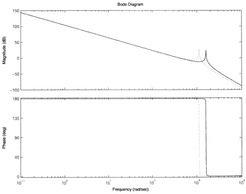
2.3.2 Damping

A very deterministic way of adding damping in belt drives is yet an area that could be

explored more. Damping has a key role to play on changing the dynamical behaviour of the system and hence impact the performance of the system. We see the effect of damping on the transfer functions in the Fig. 2-5. Damping affects the maximum achievable bandwidth and the degree of robustness of the system. We discuss this in detail in the Section 2.5.

2.4 Three D.O.F. Model to Include the Pitch Mode

of the Carriage

The belt mounts onto the carriage at a height above the center of mass. Hence, in addition to the force transmitted to the carriage, there is a torque. This torque causes the pitching motion of the carriage. Depending on the moment stiffness of the air bearings, the natural frequency of this mode could be very high or of the same order as that of the axial resonance. This could affect the closed-loop performance. The carriage can be modeled as a two-degree-of-freedom system with a translation and rotation. We are not accounting for the yaw and roll modes. A schematic of the model is shown in Fig. 2-6. We are assuming that the natural frequencies for the roll and yaw motions of the carriage remain the same even after coupling with the rest of

(25)

the system. We will derive these values also at the end of this section.

2.4.1 Equations of Motion

J101 + KR(ROi- X2- a ) + CR(ROi -: 2 - a) = T (2.11)

mf2 + K(x2 + aO - R01) + C1(- 2 + a6 - R01) = 0 (2.12)

I 1

+

Ka(x2+ a0

-

R01)+ C1(_22+

aO - RO1) + M,0 =

0 (2.13)

Here, 01, X2, and 0 represent the angle of rotation of the drive, translation of the

carriage, and the pitching angle of the carriage respectively. Now, we can develop a state space model for this dynamical system with three degrees of freedom. The state variables are the three displacements and the three velocities. Hence, we have the following

Y1 = 01; Y2 = 61; Y3 = X2; y4 = Y2; Y5 - 0; Y6

(2.14)

2.4.2 Eigenvalues and Eigenvectors

We write the dynamical equations (Eqs. (2.12) - (2.14)) in the following form.

y = Ay + Bu (2.15)

z = Cy + Du (2.16)

The eigenvalues of matrix A represent the natural frequencies of the system and the eigenvectors represent the mode shapes. We have not derived closed-form expressions for the three-degree-of-freedom model as in the two-mass model that we presented in Section 2.2. Using the values for various quantities from Table 2.1, we use MATLAB and solve the equations numerically to obtain the eigenvalues and eigenvectors. The predicted modes are 0 Hz, 226 Hz, 441 Hz. The rigid-body mode of the system is the 0 Hz mode. Table 2.2 shows the relative phases of the three degrees of freedom. From the relative phases of the three degrees of freedom, we deduce the mode shapes for the three modes.

(26)

Table 2.2: Mode shape -eigenvectors

The mode at 0 Hz is the rigid-body mode, when everything is moving in phase. As we go to higher frequencies, we find that the carriage's translation becomes out of phase with its rotation and drive's rotation at 226 Hz. At 441 Hz, the drive is out of phase with the carriage's degrees of freedom.

2.4.3 Transfer Function

The transfer function representations can be obtained by taking Laplace transforms of equations of motion. From the state space model (Eqs. (2.15) and (2.16)), we obtain the transfer function H(s) given by

H(s) = C(sI - A)- B + D _(2.17)

This works for most SISO systems. The matrices are

A

-/

₀

KR 2 J

0

KR m

0

KaR 7P_ 1 J 0 CIR m 0 CaR 'p

0

KR Ji 0 K m 0 Ka 0 CIR J 1 m 0 _P1

0

KaR J

0

Ka m

0

(Mp+Ka2 ) 'p

0

CiaR Ji

0

Cia m 1 Cia 'p (2.18)

I

Frequency r01 = ryi X2 = Y3 aO = ay5

magnitude phase magnitude phase magnitude phase

0 Hz 2.8488 x 10-2 90 2.8488x 10 2 _{90 8.0219}

x 10-6 90

226 Hz 2.0081x 10-5 180 2.5012x 10-7 0 1.0211x IO-7 180

(27)

0 1 B 0 (2.19) 0 0 0

For the case where the sensor and the actuator are collocated, the measured output

variable is 01, i.e., z = yi. Therefore,

C = 1 0 0 0 0 0 (2.20)

D = 0 (2.21)

The Bode plots corresponding to the collocated and noncollocated transfer functions are as shown in Figs. 2-9 and 2-10.

2.4.4 Roll and Yaw Modes

In the 3 d.o.f. model, we have modeled the pitch mode. But the carriage has yaw and roll modes also. The roll motion is orthogonal to the direction of travel of the carriage. Though the yaw motion has a projection in the axial direction (direction of travel), we have not included it in the model assuming that there is no significant change in the natural frequency of this mode when added to the rest of the system. Therefore, we estimate the natural frequency for the yaw and roll motions of the carriage treating it as a rigid body. The natural frequency for these motions is given

by

1 K(2.22) 2 ir I!

Km is the net moment stiffness provided by the air bearings for the roll or yaw motion of the carriage. Km depends on the configuration.

Km K l2 _{+ Kil} 2 _(2.23)

(28)

Table 2.3: The rigid body modes

There are 2 pairs of air bearings preloaded against each other and they are separated

by a distance of l. Hence, the summation of two terms K₁11.2 The inertia is the

moment of inertia of the carriage about the corresponding axis of rigid-body rotation of the carriage. The Table 2.3 lists the calculated theoretical values for the rigid body modes of the carriage.

2.5 Bandwidth of the Belt Drive

The classical definition of bandwidth is the maximum frequency at which the output of a system will track an input sinusoid in a satisfactory manner. The closed loop transfer function is given by

Y(s) G(s)H(s)

R(s) 1 + G(s)H(s)

A plot of this would have a value of 1 at low excitation frequencies and a value

G(s)H(s) at higher excitation frequencies. The frequency which marks this tran-sition is the bandwidth. For systems that have a continuous roll-off (low-pass filter behaviour), the cross-over frequency is a good approximation for the bandwidth of the system. In general, the cross-over frequency is defined as the frequency at which the gain is 0 dB or the magnitude is 1.

2.5.1 Collocated Control

We are interested in precisely positioning the payload (or) the carriage i.e., m2. To

achieve this, we can either use

Stiffness Inertia Natural Frequency

Yaw 1.5608 X 106 Nm 0.4779 Kg-M2 288Hz

Pitch 1.5128 X 106 Nm 0.1982Kg-M2 439Hz

Roll 3409420 Nm 0.5241Kg-m2

(29)

1. Collocated control: Feedback from the rotary encoder mounted on the motor

shaft (drive pulley).

2. Noncollocated control: Feedback from the linear encoder reading the posi-tion of the carriage in the direcposi-tion of travel or axial direcposi-tion.

There are some limitations in using collocated control to precisely position the car-riage.

1. Going by the definition of the bandwidth in Section 2.5, we can deduce that

the collocated control can theoretically give an infinite bandwidth precision machine i.e., the carriage will track the input over all frequencies. But this is

not really true. The collocated transfer function is given by 0/. But, we are

interested in X2 or the position of the carriage (M2). Therefore, we look at

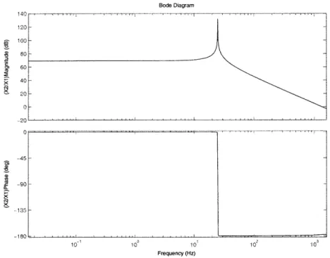
the transfer function X2/X1, the ratio of the carriage position X2 and motor

position X1. This transfer function is shown in the Fig. 2-8. We see that the

roll-off behaviour starts after the peak in the magnitude plot, which occurs at

the frequency k/rm2. This means that the carriage position does not follow

the input signal beyond this frequency. Hence, the frequency range is limited

to this frequency. The frequency k/m 2 is the frequency of the zero of the

collocated transfer function shown in Fig. 2-2.

2. (Refer to Fig. 2-7) The disturbance rejection transfer function X2

/D

looks

similar to the transfer function in the Fig. 2-8. The roll-off in the transfer

function means that the disturbances get amplified, and is not desirable.

3. Microslip between the belt and the pulley leads to a cumulative error. Due to

this error, it is difficult to determine the position of the carriage from the rotary encoder signal.

Therefore, it is difficult to achieve precise positioning of the carriage through collocated control. In the next section, we present a discussion on the maximum achievable bandwidths through noncollocated control.

(30)

2.5.2 Noncollocated control

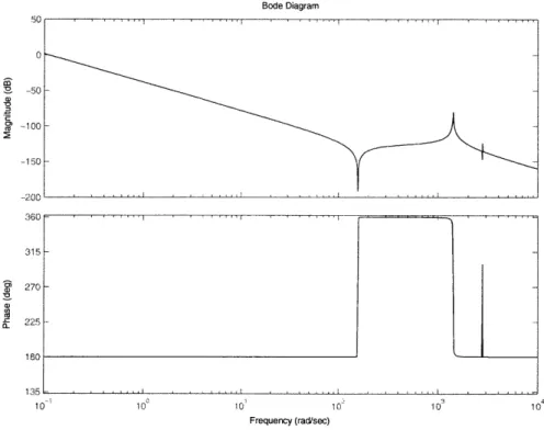
Applying the definition of bandwidth in Section 2.5 to the noncollocated transfer function, we have several possible cross-over frequencies as shown in the Fig. 2-3.

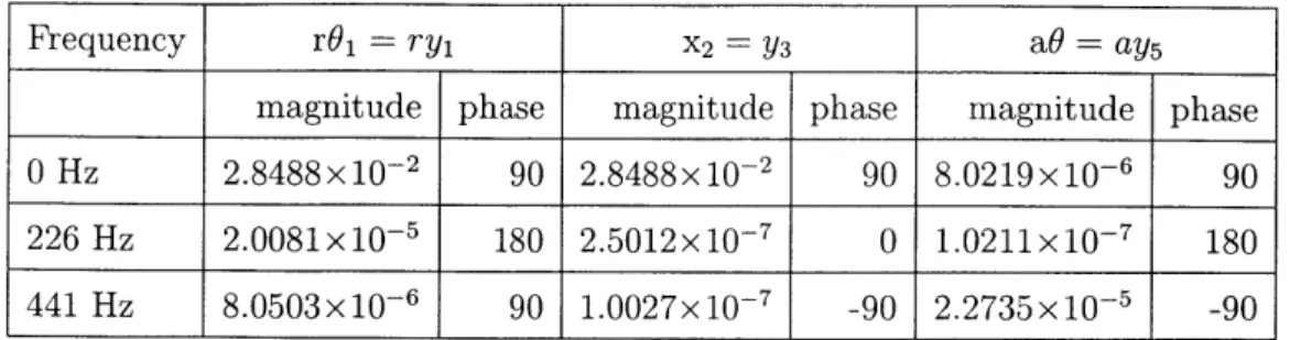
Of these 5 different crossovers possible, crossover of type 2 is the most practical.

We present arguments supporting this optimality of crossover of type 2 in the next section. Hence, as a rule of thumb, "Draw a line from the resonant peak and locate

the frequency at which it intersects the transfer function. This is the bandwidth of the system". But this crossover of type 2 is not realistic due to robustness issues which is the topic of the next section.

2.5.3 Robustness

Detailed discussions on the detrimental effects of cross overs of type 3 are presented in [3]. _{We will briefly summarize results to emphasize the fact that one cannot}

conclusively derive results on stability by just looking at the Bode plots. Nyquist plots give a more complete picture of stability and the stability margins. These are important to get insights about rather abstract mathematical definitions of stability robustness, the small gain theorem, and so on, which are the foundations of robust control. In Fig. 2-11, unit circle intersects the loop transmission at three points. These are the three crossover frequencies corresponding to type 2, 3, and 4 crossovers shown in Fig. 2-3. Going by Bode plots in Fig. 2-3, it appears that at points B and

C, gain is unity and the phase is less than -1800. Hence, we could say that the system

is unstable. But, Nyquist criterion for stability when applied to a crossover of type

3 shows that the system is stable always since the loop transmission L = GHdoes

not encircle the -1 point. Hence, it appears that crossover of type 3 gives us higher bandwidth. But, due to uncertainties in a system, crossover frequency of type 3 does not work in reality. We have to design systems with robustness, i.e. systems that continue to perform satisfactorily even in the presence of uncertainties. The stability problem in robust control is about designing a controller that works for a set of plants rather than a given plant. This is a more realistic description of a physical

(31)

system as we often do not have an exact description of the plant. Hence, our metrics for performance and stability should always address robustness issues. To give an example, our description of damping of the system is not always accurate. If we use a theoretical value for damping and estimate the bandwidth using our rule of thumb (cross over of type 2) and it turns out in practice that we overestimated the damping, we end up making a cross over of type 3. But, cross over of type 3 is detrimental as it has a very little phase margin and hence not robust. The familiar solution to this problem is to add a lead compensator to increase the phase margin. Adding a lead compensator will add phase at the cross over but make the system unstable at resonance, i.e, loop transmission will encircle the -1 point in the nyquist diagram (refer to Fig. 2-12). The next best possible cross over would be of type 2. But the crossover of type 2 is also not very robust, if our plant model had some uncertainties. For example, how do we accommodate an overestimated value of damping?. Hence we introduce a gain margin at resonance. The resonance gain margin (RGM) is defined as the factor by which the loop transmission has to be multiplied without resulting in multiple cross overs at resonance. This is shown in Fig. 2-11. For a detailed discussion on robust stability, the reader is referred to Dahleh [2] and Doyle [6]. In summary, crossover of type 1 works best in reality. The stability margins are important because our ultimate objective is to be able to derive synthesis rules for designing a high bandwidth belt-driven servomechanism. In other words, the designer should be able to size the various components like belt, motor inertia etc., to meet the performance criteria such as bandwidth. Hence, we have to derive closed-form expressions for maximum achievable bandwidth for a robust belt-driven system.

2.5.4 Crossover of Type 5

The phase has already dropped to -3600 at the crossover frequency (Type 5 in Fig.

2-3). To keep the system stable, we need to add a phase of atleast 1800 which would

lead to high gains, often leading to actuator saturation. This point can be explained as follows. A phase increase of 1800 would require a compensator with two zeros ahead of the resonance. This compensator would be accompanied with two poles and

(32)

hence akes te form(8+Z)2 _Ti

hence takes the form ,p . This means amplifying the input to the amplifier at the

rate of 40 dB/decade, which will lead to actuator saturation. In practice, this method rarely works.

2.6 Chapter Summary

In this chapter, we have developed a lumped-parameter model for the belt drive. We have also presented closed-form expressions for the collocated and noncollocated transfer functions. We have presented a discussion of the maximum achievable band-widths of the belt-driven system with certain robustness in the presence of uncertain-ties in the system modeling and other errors.

(33)

Bode Diagram

10 10,

Frequency (rad/sec)

Figure 2-2: Collocated transfer function

100 50 0 -50 -100 150 5 - 0-0 c 13 18 1 0 10 .4 9 10

(34)

Bode Diagram .Typ~e 1 Type 2 RGM Type 3 A Type 4 Type 5 10 10 102 Frequency (rad/sec)

Figure 2-3: Noncollocated transfer function

100 01 501 -a_CD Ca .r-CL 10 10 180 135 45 Z_CM Ca 2 0 10

(35)

Bode Diagram 100 50 -50 135 90 45 0~ 0 10 100 10 104 Frequency (rad/sec)

Figure 2-4: The effect of change in stiffness in the noncollocated transfer function

F

4

'

1 f

b

i

- -

i

r -L

CO 2

(36)

Bode Diagram 100 50 0 .50 a 135 90 45 10 10 10 10 Frequency (rad/sec) 10 3ed 104

Figure 2-5: The effect of damping in the noncollocated transfer function

m

1

X2

a6

Figure 2-6: Three-degrees-of-freedom model 50I

Drop in resonant -peak due to increa damping

-Ii

CO 2

(37)

motor carriage

distu bance disturbance

D(s)

X(s) + + Y(s)

+ H(s) G(s)

F

Figure 2-7: Closed-loop servomechanism

Bode Diagram

10 10 103

Frequency (Hz)

Figure 2-8: Transfer function x_xi

140 10 80, 60 401 2i -45 -90 135

(38)

-Bode Diagram 50 3150 31 -270 - 22-180 135 -10 10 10 10 Frequency (rad/aec)

(39)

Bode Diagram -50 100 -Q> 2 -20r- 250--225 -270 -315 10 10 10 10 10 10 Frequency (rad/sec)

Figure 2-10: 3 DOF model - noncollocated transfer function

(40)

hn(L(jw)) Unit Circle for

Unit Circlefa ,Cossover (3):

Unit Circle fot

Crossover (4)

Figure 2-11: Nyquist representation of crossover frequencies, Varanasi [3]

(41)

Incg2asing _has

(42)

CMIL Robustness Margin PM 2sin M/2) D curve Nominal P~lant R*~(LUw)) unit eircj

Figure 2-13: Nyquist interpretation of robust gain margin (RGM) and phase margin

(43)

Chapter 3 Energy Dissipation due to Slip in

Belt Drive: Damping and Loss

Factor Estimates

3.1 Introduction

This chapter presents a model for microslip in belt drives and estimates for the damp-ing due to microslip. We characterize the dampdamp-ing by the loss factor which is defined as the ratio of the energy loss and the maximum potential energy during one cycle of harmonic motion. We are interested in understanding how the slip region varies under harmonic excitations. We explain the origin of microslip and model the slip region on the belt-pulley interface as a deformable control volume. Using the mass conservation, we obtain the rate at which the slip region changes. The size of the slip arc is given by the capstan formula. We obtain expressions for the loss factor in terms of parameters like belt preload To, the drive ratio n, the length of the drive L, the cross section A, and friction coefficient p. The loss factor estimates show that the damping one can achieve due to microslip is not very significant. The loss factor is estimated to be of the order of 10-% for a typical configuration.

(44)

3.2 Notation

#

Slip are T Tangential traction - Stress p Poisson's ratio G Rigidity modulus q Traction distribution

p Normal pressure distribution

P Normal load

Q

Tangential load

6 Tangential displacement

To Belt preload (or) pre-tension

R2 Radius of the driving pulley

R1 Radius of the driven pulley

V2 Peripheral speed of the driving pulley

V1 Peripheral speed of the driving pulley

A Area of cross section of the belt

p Density of the belt material

4

Rate of change of slip arc

p Coefficient of friction

3.3 Microslip

-

Background

The earliest investigation of slip and the associated energy loss was by Mindlin et al [7]. In this section, we will elucidate some of the results from their work. We also describe the origin of slip and a method used by Mindlin et al for estimating the energy loss due to slip. They first studied the problem where a pair of elastic bodies were pressed against each other and a small tangential force is applied across the elliptic contact surface [8].

(45)

3.3.1 Microslip and Sliding

A tangential force whose magnitude is less than the force of limiting friction, when

applied to two bodies pressed into contact, will not give rise to a sliding motion. But this force will induce tangential surface tractions which arise from a combination of normal and tangential forces; this does not cause the bodies to slide relative to

each other. When a tangential force

Q

is applied to two bodies of non-conformal

geometries (refer to Fig. 3-1) pressed against each other with a normal force P, the

tangential force

Q

deforms the bodies in shear. This causes the points on the contact

surface to have tangential displacements relative to the distant points on the bodies. There will be atleast one point which is at rest as long as there is no gross sliding

motion. But, there are points which slip even though

Q<

pP, i.e., there is some slip

even in the absence of gross-sliding. This is referred to as microslip. This slip can be mathematically expressed as

slip, s=, ={ui - 6X1} - {ux2 - x22 (3.1)

where 621 and 6x2 are displacements of points far away from the contact surface, which

are used to define the tangential compliance.

3.3.2 Boundary Conditions

In order to solve the boundary value problem of two nonconformal spheres in contact, we need to state the boundary conditions that distinguish the stick and slip regions. These boundary conditions are

stick region sx =0; = Ux1 - Ux2 = 6x1 - 6x2 (3.2)

(46)

3.3.3 Assumptions

Effect of the Tangential Force

Q

on Hertzian Distribution of Normal Pres-sure, p(x, y)

A normal force pressing the two bodies together is the Hertzian contact problem [11]. When a tangential traction exists on the contact surface, we could say that, if

the two solids have the same elastic constants, any tangential traction transmitted between them gives rise to equal and opposite normal displacements of any point on the interface and it does not affect the distribution of normal pressure predicted by Hertz theory. This is because the normal displacements due to these tractions are

proportional to the respective values of (1-2v) Therefore, we have

G

G1 _G2

Y

I v zi (X, y) = - 2v Uz2(,y (3.4)

where, uz refers to displacements in the normal direction. But even between different materials, the influence of tangential tractions on the distribution of normal pressure is generally small and it is ignored in all the analysis presented in the previous section.

Amonton's Law

Amonton's Law of static friction is applicable at each elementary area of the interface. It can be stated as

Iq(x, y)I

IQ|

p(x,

y) - _(3.5)

3.3.4 Mindlin's Solution and Results

Hence the problem of two spheres (refer to Fig. 3-1) solved by Mindlin is a boundary value problem where the tangential displacement u. and normal pressure p(x, y) are given over part of the boundary, i.e., the contact region and the three components of traction (=O) are given over the rest. The solution of this problem assuming 'no slip' through out the contact region leads to the following distribution of tangential

(47)

P

-- +Q

Figure 3-1: Two spheres in contact under normal and tangential load

traction over the surface.

T = r < a (3.6)

27ra(a 2 _- _{r2 ,}

The tangential traction is everywhere parallel to the direction of the applied force. The contours of constant tangitial traction are concentric circles. The displacement is linear and the tangential compliance is given by

1 2 - v 2 - v2

C-1-(

)

(3.7)

8a G1 G2

where v = Poisson's ratio and G = rigidity modulus. We see that at the boundary

of the contact area, i.e., at r = a, the tangential traction goes to infinity. But, we presume that the tangential traction cannot exceed p times the normal traction if there is no slip. Hence, some portion of the contact region has to slip. Assuming that there is a slip region and an adherent region, Mindlin solved the boundary value problem using the second boundary condition given by Eq. (3.3) over a part of the boundary. The following are some of his results. The inner radius of the annulus of the slip region is given by

c = a(1 - Q) (3.8)

pP

From this expression we can see that when the applied tangential force

Q

exceeds PP,

c goes to zero and gross sliding occurs, which we are familiar with. The distribution of the tangential traction on the contact surface is

3p-P 2_21

T = 2703 (a2 r2), c < r < a (3.9)

(48)

and the displacement of distant points w.r.t the uniform displacement of the adhered portion is

(2 - v)p-P

_Q

S= 3 _ [1 - (I - P)] (3.11)

16[pa (1-P_

The tangential compliance for this configuration can be derived as

dJ 2 - v

Q

1

C8 (1 - ) (3.12)

dQ 8pa pP

Note that in this solution the compliance is a function of

Q,

i.e., the Q-6 curve is

non-linear. Considering a case of cyclic loading, where the normal force is kept constant and the tangential force is varied, the expressions for the traction distributions, com-pliance for loading and unloading and displacements have been derived by Mindlin

[8]. We can see a hysteresis effect and the associated energy loss due to slip over one

cycle is given by

9( 2 - V )p2 p2 QmaT 5Qmax [1+ QMax)

{1 - (1 -- )3 - [1 + (1 - )3]} (3.13)

1OEa PP 6pQ pP

Experimental results for hard steel spheres pressed against flats are in good agree-ment with the above results and confirm the energy dissipation due to microslip [9]. In this paper, Johnson has presented the observations from the damping tests con-ducted to obtain the energy dissipation due to microslip. In the dynamic tests, he has demonstrated the marked distinctions between the microslip and gross sliding. In the regime of microslip, the oscillations are harmonic and are about an unvarying datum

position. When

Q

exceeds pP, slide ensues and unsteady non-harmonic motion is

setup. Following this work, there were other researchers who demonstrated the valid-ity of the theory proposed by Mindlin [10]. The experimental studies investigating the effect of oblique forces and their angles of inclination w.r.t. the plane of contact were by Johnson [11].

So far, we have discussed the theoretical framework for studying microslip under static conditions when the bodies are in contact and are at rest, even though the forces could be oscillating in magnitude.

(49)

3.4 Belt Drive

-

Microslip

In this section, we discuss the origin of microslip in the belt drive and derive expres-sions for energy dissipation when the system is driven by harmonic excitations. This problem is different from the microslip under static conditions that we have discussed in the previous sections. In the traction drive under study, the contact surfaces are moving relative to each other. The boundary condition that defines the slip region is different in this problem when compared with the one given by Eq. (3.3) and it is

given as A_ = 0 in the stick region. Different components of velocities occur in the

expression for slip velocity

s,

depending on the complexity of the configuration. This

includes rolling, spinning, sliding, and so on. A detailed discussion of the microslip in rolling elastic bodies in contact is done by Johnson [12].

3.4.1 Motivation

Belt-driven servomechanisms are widely employed in precise positioning applications which include semiconductor and optical industries. The most important limiting factors on the performance of these precision machines arise from the inherent dy-namics of the system. Hence, in the design of such servomechanisms, a complete understanding of the dynamics of the system is essential. This would help us derive synthesis rules for the design of such drives to achieve high bandwidth, accelerations, and speeds. Damping plays a very important role in the stability and performance of the belt-driven servos. For example, a well-damped resonance peak would help us achieve high crossover frequencies and hence high bandwidth [3]. In a belt drive, there is some energy loss when the belt slips on the pulley [12]. Researchers have worked on modeling the slip and obtaining the power loss and efficiency in the context of power transmission [13, 14]. These researchers study the mechanics of a steadily rotating belt drive. Our objective is to understand the mechanics of energy dissipa-tion under harmonic excitadissipa-tions and derive an analytical expression for the loss factor in the belt drive.

(50)

3.4.2 Loss Factor

-

Definition [15]

Loss factor is a measure of the damping in a system. A vibrating system may have different types of energy dissipation mechanisms and their mathematical descriptions in terms of the damping force are quite complicated. Instead, we can characterize damping by the amount of energy dissipated under steady harmonic motion. The most common measure of this dissipation is the loss factor q, which is formed by taking the ratio of the average energy dissipated W per radian to the peak potential energy U during a cycle. That is

w

2WU (3.14)

3.4.3 _{Origin of Microslip in Belt Drives}

Due to the compliance of the belt, the belt stretches. The tight side has a higher tensile force and hence stretches more than the slack side. This explains the origin of the microslip in the belt drive. To develop a complete picture of how the slip occurs and locations where the belt slips, we present the following arguments, discussed

in detail by Johnson [11]. Consider an infinitesimal element of the belt dx. Let

the tensile strain experienced by that element be c. Using the familiar constitutive relation

= Ec (3.15)

dl (1 + E)dx (3.16)

Differentiating the above expression w.r.t. time, we obtain

dl

V =dt

dx -dx

(1 + E) _dt + _{E dt})(3.17)

where L defines the unstretched velocity of the belt. This clearly indicates that the tight side of the belt moves faster than the slack side of the belt. Now we obtain expressions for the speeds of the belt on the tight side and the slack side as V and

(51)

V2 respectively given by TO + T1 dx FA= 1+ - (3.18) E A dt

T - T

1

dx

V2E (+ ) (3.19) E A dt

Consider the instant of time when the direction of motion of the driven and driving pulleys are as shown in the Fig. 3-2 The frictional traction pulls the belt forward on the driven pulley and it opposes the belt motion on the driving pulley. We also know that the direction of the frictional traction is such that it opposes the direction of slip. Therefore,

1. The driving Pulley must be moving faster than the belt in the slip arc.

2. The driven Pulley must be moving slower than the belt in the slip arc.

Hence we deduce that the belt adheres where it runs onto the pulley and it slips as it leaves the pulley on both driver and driven pulleys.

3.5 Model: Deforming Control Volume

We are interested in estimating the energy loss during one cycle of harmonic motion of the form eiwt. When the direction of rotation changes, the location of the stick arcs shift to satisfy the condition stated at the end of the previous section, i.e., the belt adheres where it runs onto the pulley. The slip arcs are expected to vary with time as the harmonic input varies from a maximum to a minimum. We propose a deforming control volume model to accommodate the above variations in slip arcs. The control volume is as shown in the Fig. 3-2.

3.5.1 Slip Rate: Mass Conservation

Applying the continuity equation for this deformable control volume which is moving relative to the pulley, we obtain

ddr +

I>pV.VdQ

(3.20)

Dynamics of belt-driven servomechanisms : theory and experiments

Dynamics of Belt-Driven Servomechanisms

Theory and Experiments

by

Dhanushkodi D. Mariappan

Bachelor of Technology (B.Tech), Mechanical Engineering

Indian Institute of Technology, Madras 2001

Submitted to the Department of Mechanical Engineering

in partial fulfillment of the requirements for the degree of

Master of Science in Mechanical Engineering

at the

MASSACHUSETTS INSTITUTE OF TECHNOLOGY

June 2003

@

Massachusetts Institute of Technology 2003. All rights reserved.

Author ...

...

Department of Mechanical Engineering

May 23, 2003

Certified by...

...

...

Samir A. Nayfeh

Assistant Professor

sis Supervisor

Accepted by ...

...

Ain A. Sonin

Chairman, Department Committee on Graduate Students

JUL 0 8 2003

I

/

i')

a

Dynamics of Belt-Driven Servomechanisms

Theory and Experiments

by

Dhanushkodi D. Mariappan

Abstract

Acknowledgment

Contents

List of Figures

List of Tables

Chapter 1

Introduction

1.1

Servomechanisms: Feedback

-

Performance

Cri-teria

1.1.1

Parameters of Performance

1.1.2

Design for Closed-Loop Performance [3]

1.1.3

Limitations

1.2

Contributions

Chapter 2

Modeling the Axial Dynamics of

the Belt Drive

2.1

Introduction

2.2

Modeling the Dynamics

2.2.1

Model for the Belt Drive

E

2.2.2

Equations with Damping Terms Included

±S2E

+

E(s)

MS2

+

jw,

2.3

Effect of Varying the Stiffness and Damping

2.3.1

Stiffness

₀