Dynamics of a continuum characterized by a non-convex energy function

Dynamics of a

Continuum Characterized

by a Non-convex Energy

by

Yier Lin

M.S. Mechanical Engineering

Northeastern University

(1988)

SUBMITTED TO THE DEPARTMENT OF

MECHANICAL ENGINEERING

IN PARTIAL FULFILLMENT OF

THE REQUIREMENTS FOR THE

DEGREE OF

DOCTOR OF PHILOSOPHY IN MECHANICAL ENGINEERING

at the

MASSACHUSETTS INSTITUTE OF TECHNOLOGY

June 1993

©

1993 Massachusetts Institute of Technology

All rights reserved

Signature of Author

Department of Mechanical Engineering

April 10, 1993

Certified by

Rohan Abeyaratne

Associate Professor, Department of Mechanical Engineering

Thesis Supervisor

Accepted by

Ain Ants Sonin

Chairman, Graduate Thesis Committee

ARCHIVES

MASSACHUSETTS INSTITUTE

Function

Dynamics of a Continuum Characterized

by a Non-convex Energy Function

by

Yier Lin

Submitted to the Department of Mechanical engineering on April 12, 1993 in partial fulfillment of the requirements for the Degree of Doctor of Philosophy in

Mechanical Engineering

Abstract

This thesis investigates the dynamics of nonlinearly elastic bars when the energy function that characterizes the material is a non-convex function of strain. Such energy functions have been used, for example, to describe the behavior of solids that can undergo stress-induced phase changes. Dynamic problems for such a material typically involve two types of prop-agating strain discontinuities, phase boundaries and shock waves. The classical continuum theory of dynamics involves the field equations and jump conditions stemming from mo-mentum balance and kinematic compatibility together with the entropy inequality. In the setting of this theory, even one-dimensional problems often possess an infinite number of so-lutions when the energy function is non-convex, and the theory is therefore not well-posed. The theory must be supplemented with additional information from the physics of phase

transitions.

In part A, we study the propagation of a phase boundary separating a stable phase from a metastable phase. We consider a general non-convex material and show that the propagation of such a phase boundary is controlled by its kinetics.

In part B, we consider a phase boundary separating a stable phase from an "unstable phase". In this case we show that the propagation is controlled by inertia rather than kinetics.

In part C, we model and analyze a plate impact experiment for this class of materials. The results are compared with experimental observations on limestone undergoing the calcite

I -* calcite II transition.

Thesis Supervisor: Dr. Rohan Abeyaratne

Acknowledgments

My deepest appreciation goes to my thesis supervisor, Professor Rohan Abeyaratne for

his generous support and unlimited patience throughout the course of this research. His enthusiasm and dedication constituted a very important factor for the conclusion and the achievements of this work. Without his guidance, technical assistance, and encouragement, this thesis would not have been possible.

I am also greatly indebted to the other members of my thesis committee, Professors David

M. Parks and Triantaphyllos R. Akylas. Their comments and suggestions for improving this thesis are greatly appreciated.

I would like to express my appreciation to my colleagues and friends in the Mechanical

Engineering Department. Especially I would like to thank Sang-joo Kim for the many conversations we had. Special thanks also go to Xiaojun Liu and Yunpeng Gu for their insightful suggestions that were very valuable to me in presenting my thesis defence.

To my parents, Dejiang Lin and Suzhen Zhang, I owe the unconditional love they have given me and the sacrifices they have made for me. I also would like to thank my brother, Li Lin, who motivated me to study at MIT. Special thanks go to my uncle, Tak-ming Lam, and aunt Ulla Lam, for their moral support and encouragement.

My wife, Jihong Zhang, has been my source of strength. This thesis would never have

been completed without her love, patience and understanding. It was her unfailing confidence in my ability to attain my doctoral degree that inspired and motivated me to continue in times of doubt. Moreover, I am forever indebted to her for giving birth to our daughter, Elizabeth. Elizabeth has given a new meaning to our lives.

This work was supported by the U.S. Office of Naval Research to whom we express our thanks.

Contents

Abstract

Acknowledgments

1 General Introduction

1.1 General Description . . . . 1.2 Review of Continuum Modeling of Reversible Phase Transitions . . . . 1.3 Present Thesis . . . .

PART A. Propagation of an Interface into a Metastable Phase

2 Introduction

3 Basic Equations

4 Material; Local Properties of Discontinuities

5 The Riemann Problem: Construction of Solutions

5.1 Form ulation . . . .

5.2 The Structure of Admissible Solutions to the Riemann Problem . . . .

6 Explicit Solutions to the Riemann Problem

1

3

10 10 12 15

17

18 22 25

33

33

36

42

6.1 Solutions Involving No Phase Change . . . .

6.2 Solutions Involving a Phase Change . . . .

6.3 Summary of All Solutions . . . . 7 Kinetics and Nucleation

PART B. Propagation of an Interface into an Unstable Phase

8 Introduction

9 Equilibrium States 10 Quasi-static Motions

11 The Regularized Theory: A Traveling Wave Problem

11.1 Construction of the Traveling Wave Problem . . . .

11.2 Solutions to the Taveling Wave Problem . . . .

12 The Dynamic Theory

12.1 B ackground . . . . 12.2 The Riemann Problem . . . .

12.3 The Structure of Admissible Solutions to the Riemann Problem . . . .

12.4 Solutions to a Riemann Problem . . . .

13 Conclusions

PART C. An Application: The Impact Problem

14 Introduction 42 46 52 58

62

63

67 73

77

77 80 88 88 90 91 95 103

104

105

15 Formulation of Impact Problem

16 Local Properties at a Phase Boundary 17 Two Preliminary Problems

17.1 The Signalling Problem . . . . 17.1.1 The Initial Data in the Low-strain Phase . . . .

17.1.2 The Initial Data in the High-strain Phase . . . . 17.2 The Riemann Problem . . . . 17.2.1 A Riemann Problem Involving Two Distinct Materials 17.2.2 A Riemann Problem for a Two-phase Material . . . . . 18 The

18.1 18.2

Impact Problem: Construction

No Phase Change in the Specimen With phase change in the specimen

of Solution

. . . .

. . . .

. . . .

. . . .

. . . .

. . . .

19 Results and Discussion

19.1 Non-dimensionalization . . . . 19.2 Results . . . . 19.3 Experimental results . . . . 19.4 Comparison . . . . 20 Concluding Remarks

References

109 114 119

119

120 124 125 125

127

132

133

134 141 141 143 145 146 154

159

List of Figures

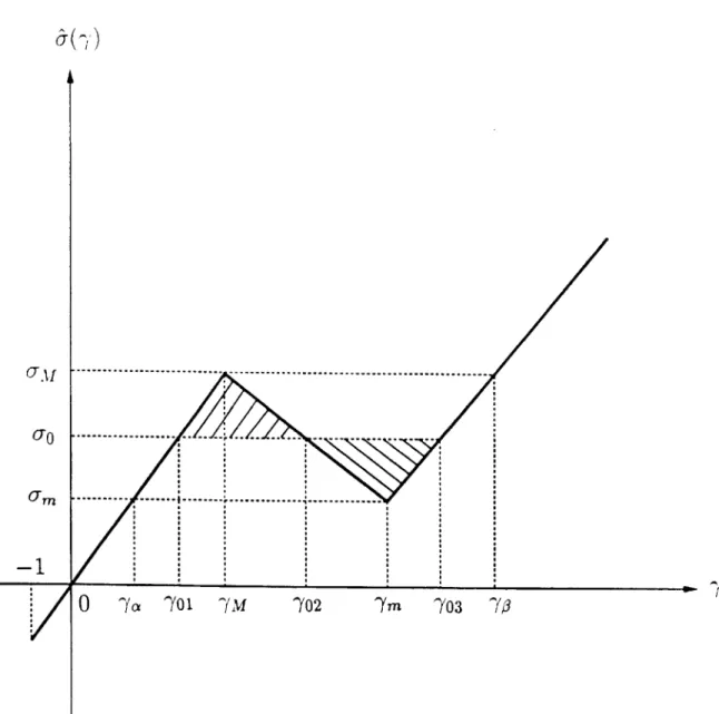
4.1 Stress-strain curve . . . .

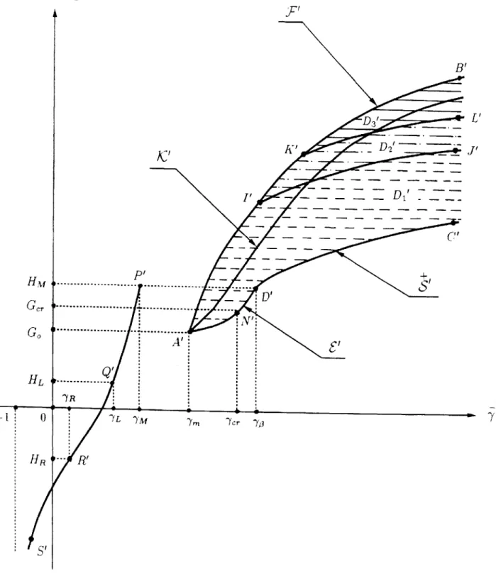
4.2 The regions Fj in the (7,7)-plane . . . . 4.3 Admissible images of Fj in the (., f)-plane . . . .

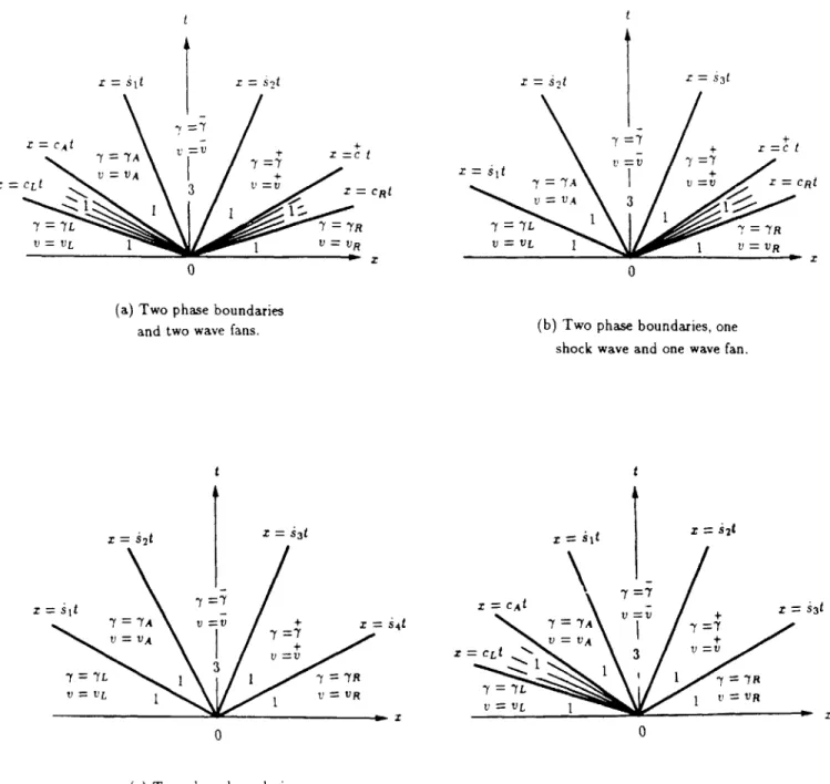
5.1 General form of solutions to the Riemann problem . . . .

6.1 Form of solutions to Riemann problem without phase change

6.2 Form of solutions to Riemann problem with phase change . .

6.3 The regions Di in the (7,7)-plane . . . .

6.4

The

(1,7R -

VL)-plane . . . .

8.1 Free-energy versus strain at temperature perature ... ...

above and below

. . . .

the critical 9.1 9.2 Stress-strain curve . . . . The (6, o-)-plane . . . .

10.1 The (6, o)-plane. Admissible directions .

11.1 The (.,7)-plane . . . .

12.1 Assumed form of solutions to the Riemann 12 .2 . . . . problem

30

31 32 . . . . 41 54

55

56 57

tem-66

71 72

76

87

100 101

. . . .

. . . .

12.3 Form of solutions to Riemann problem . . . 102

14.1 Plate im pact assem bly . . . 108

15.1 Stress-strain curve . . . . 112

15.2 Initial conditions, boundary conditions and interface conditions of impact problem . . . 113

16.1 The (7,4)-plane . . . . 117

16.2 The (A,f)-plane . . . . 118

17.1 Form of solutions to the signalling problem . . . . 128

17.2 The (A, o-B)-plane . . . 129

17.3 Form of solutions to Riemann problem involving two distinct materials . . . 130

17.4 Form of solutions to Riemann problem involving a single material . . . 131

18.1 Wave pattern without phase change . . . 137

18.2 Velocity at free-end of specimen versus time for the case without phase change 138 18.3 Velocity at free-end of specimen versus time when both impactor and specimen are composed of the same material . . . 139

18.4 Wave pattern with phase change . . . 140

19.1 Wave pattern without phase change . . . 148

19.2 Velocity at free-end of specimen involving no phase change versus time . . . 149

19.3 Wave pattern with phase change . . . 150

19.4 Velocity at free-end of specimen involving a phase change versus time . . . . 151

List of Tables

19.1 Comparision between exact and approximate solutions . . . 153 19.2 Grady's experimental results . . . 153 19.3 Results of present calculation . . . 153

Chapter 1

General Introduction

1.1

General Description

Many alloys occur in more than one crystal structure, each crystal structure being termed a phase. One phase exists under certain conditions, while another exists under different conditions. Such materials can transform from one phase to another when they are subjected to an appropriate change in either stress or temperature. Examples of such materials are the shape-memory alloy NiTi, the ferroelectric alloy BaTiO3, ferromagnetic alloy FeNi and

the high-temperature superconducting ceramic alloy ErRh4B4.

Consider for instance the class of In-Ti alloys described by Burkart and Reed (1953). These alloys can exist in two solid phases. A cubic phase (austenite) is preferred at a stress below the transformation stress oo, and a tetragonal phase (martensite) is favored above it. When a specimen of austenite is subjected to a monotonically increasing stress, the martensite phase is nucleated at the "martensite start stress" oM.( ao). The specimen now

consists of a mixture of both austenite and martensite. The coexistent phases are separated from each other by one or more interfaces-phase boundaries; the phase boundaries are said to be coherent in the sense that the deformation is continuous across them even though the deformation gradient is not. As these phase boundaries propagate, the entire specimen will

eventually be converted into martensite. If the stress is now decreased, the whole process is reversed, with the martensite to austenite transformation being initiated at the "austenite start stress" O'A,5( oo). This is a reversible or thermoelastic phase transition. The values of

the nucleation stresses u, and 0

A, as well as the transformation stress 0o depend critically

on the alloy composition, the heat treatment and the temperature (Otsuka (1986)).

The mechanical properties of a material sometimes can be improved by exploiting a phase transformation. For example, if steel in its austenite phase is cooled to below the martensite nucleation temperature, the martensite can precipitate as finely dispersed particles. Since these closely spaced precipitates of stronger martensite can obstruct dislocation motion, there is an increase in the strength of the steel (e.g. Cottrell (1967)). Another example is the toughening of certain ceramics (Evan et al (1986), Green et al (1988)). In PSZ (partially stabilized zirconia), sub-micron sized zirconia particles in their tetragonal phase are dispersed within a zirconia matrix which is in its cubic phase. When sufficiently stressed, the tetragonal zirconia transforms into its monoclinic phase, and there is an accompanying order of magnitude increase in the toughness of the material (Evan et al (1986)). A third example is provided by the thermoelastic behavior of shape memory alloys. Since these materials have very different stress response on different ranges of temperature, it has been possible to design a material to possess various desired mechanical responses at various

chosen temperatures (Schetky (1979)).

Many phase transitions, such as those occurring in steel, are not reversible, the de-formation associated with the transde-formation being coupled with plastic dede-formation, e.g.

1.2

_{Review of Continuum Modeling of Reversible Phase}

Transitions

Various aspects of the theory of finite thermoelasticity associated with reversible phase trans-formations in crystalline solids have been studied in a number of recent papers; see for exam-ple Ericksen (1980,1986), James (1986) and Pitteri (1984). For a thermoelastic material, the Helmholtz free-energy function 0 depends only on the deformation gradient tensor F and the temperature 9: 0 = _{#(F, 9). If the stress-free material can exist in more than one phase,}

then the energy function $ must have multiple energy-wells, each well being associated with a phase. In particular, for a two-phase material, one minimum corresponds to austenite and the other to martensite. At the transformation temperature OT, the two energy minima have the same value. For 9 < OT, the martensite minimum is smaller; in this case, we speak

of the martensite as being stable and the austenite as being metastable. For 9 > OT, the

austenite minimum is smaller; thus the austenite is stable and the martensite metastable. As the stress-free material is cooled or heated, it often transforms between the martensite and the austenite. In the presence of stress S, one must consider the potential energy func-tion G = _{G(F, S, 9) involving multiple energy-wells where S is the first Piola-Kirchhoff stress}

tensor. In this case, the material can transform from one phase to another if it is stressed or heated by a suitable amount.

Since the deformations on either side of a phase boundary are distinct, and there is a finite discontinuity in the deformation gradient tensor across a phase boundary, the constitutive relations which can be used to model phase transitions must have the capability of sustain-ing such deformations. The occurrence of such deformation fields is closely related to the changing of type of the (displacement) equations of equilibrium from elliptic to non-elliptic. The interpretation of these ellipticity conditions has been a source of considerable difficulty.

Abeyaratne (1980) showed in two-dimensions that strong ellipticity is essentially equivalent to the convexity of the potential energy. The analogous issue within the three-dimensional theory was investigated by Rosakis (1990).

Continuum mechanical studies of reversible phase transitions have been focused on two basic issues; the first is related to energy minimizing deformations corresponding to the stable configurations of a body, the second is associated with the non-equilibrium evolution of a body towards such stable configurations through intermediate states of metastability.

Ericksen (1975) studied the deformation of a bar composed of a two-phase material. In this one-dimensional setting, he showed that, for certain values of the prescribed elongation, the stable configuration of the bar involves a mixture of coexistent phases. In seeking such an absolute minimizer, he showed that an additional jump condition, the "Maxwell condition", must hold at the phase boundary. The related question of the minimization of energy in the three-dimensional theory was examined by James (1981), Abeyaratne (1983) and Gurtin

(1983); they derived a supplementary jump condition (analogous to the Maxwell condition)

which should hold at a singular surface if the equilibrium field is to be stable.

Silling (1988) examined certain implications of the Maxwell condition within the setting of anti-plane shear of a two-phase material. He observed that, in many reasonable boundary-value problems, the Maxwell condition cannot be satisfied exactly, and that it can only be satisfied in the sense of a limit of an infinite sequence of increasingly chaotic deformations. Ball and James (1987) examined this same issue in three dimensions and showed that the absolute minimizers of energy can involve a stable configuration of fine mixtures of phases; in particular, they studied an austenite/twinned martensite interface in detail, and showed that the consequences of their theory are in agreement with the crystallographic theory of martensite.

The usual continuum theory of thermoelasticity, though adequate for describing the en-ergy minimizing deformations of the two-phase material, does not, by itself, characterize quasi-static or dynamic processes of a body involving phase transitions. This can be il-lustrated by the lack of uniqueness of solution to certain initial-boundary-value problems; Abeyaratne and Knowles (1988, 1991).

Quasi-static or dynamic processes generally involve states that are merely metastable and so fall under the category of "non-equilibrium thermodynamic processes." Considerations pertaining to the rate of entropy production during such a process naturally leads to the notation of the driving force (or Eshelby force) f acting on a phase boundary, Abeyaratne and Knowles (1990); see also Eshelby (1956), Knowles (1979), Rice (1975). The theory of non-equilibrium processes can then be used to argue for the need for a constitutive equation - a kinetic law - relating the propagating speed V, of the phase boundary to the driving force

f and the temperature 9: V, = V,(f, 9). The kinetic law controls the rate of progress of the

phase transition; the importance of a kinetic law in the description of phase transitions in solids has long been recognized in the materials science literature, e.g. Christian (1975); in fact, some, though not all, micro-mechanical models of kinetics lead to the kinetic laws of the form V, = V,(f, 9). The kinetic relation controls the progress of the phase transition once it

has commenced. A separate nucleation condition is required to signal the initiation of such a transition. This is analogous to the roles played by a flow rule and a yield condition in continuum plasticity theory. A general discussion of nucleation theory in phase transitions, from a materials science point of view, may be found in Christian (1975). Thus a complete constitutive theory which is capable of modeling processes involving thermoelastic phase transitions consists of three ingredients: a Helmholtz free-energy function, a kinetic relation and a nucleation criterion.

Most multi-dimensional problems associated with phase transitions must be solved nu-merically. Collins and Luskin (1989) have studied energy minimizing deformation in this way, and Silling (1988) has studied questions related to propagation. Molecular dynamics simulations have also been carried out, e.g. Yu and Clapp (1989).

1.3

Present Thesis

Many martensitic phase transformations take place at very high rates; sometimes, phase boundaries move at speeds which are of the order of the shear wave speeds in the solid (Bunshak and Mehl (1952)). According to Grujicik, Olson and Owen (1985), reported mea-surements of phase boundary velocities vary widely, from values small enough to permit direct optical observation to values approaching the speed of shear waves in the parent phase of the material. Dynamic effects would therefore be very important in the study of such phase transformations.

From the theoretical point of view, there are a number of important questions pertaining to the dynamics of a material undergoing phase transformations. In the mathematical study of systems of conservation laws in one space dimension (see, for example, Dafermos (1983,

1984), Lax (1973)), it is known that the solution to an initial-value problem, subject to the entropy inequality, is unique, provided that the curvature of the underlying stress-strain relation is always of one sign and that it is monotonic (Oleinik (1957)). However, in the absence of monotonicity and convexity (or concavity), the entropy inequality is not strong enough to secure uniqueness. This is, of course, precisely the class of materials that is of interest in studying phase transformations.

The purpose of the present thesis is to explore the effects of inertia on the continuum theory of reversible phase transitions. In parts A and B of this thesis we consider theoretical

issues related to the propagation of a phase boundary. Having thus addressed the formulation of dynai. ic problems, in part C, we turn to a specific dynamic problem, viz. an impact problem. More specific introductions to each of the issues studied in the three parts A, B,

PART A:

Propagation of an Interface

into a Metastable Phase

Chapter 2

Introduction

In the simplest one-dimensional theory describing the longitudinal motions of an elastic bar, one employs a pair of conservation laws associated with momentum balance and kinematic compatibility. When the motion of the bar involves a propagating strain discontinuity, it is subject to a pair of jump conditions associated with these conservation laws. In addition, the second law of thermodynamics requires that the dissipation associated with the moving discontinuity be non-negative, a condition usually referred to as the entropy inequality.

The character of the material of the bar enters the conservation laws and jump conditions through the stress-strain relation a-= &(-y). If the material of the bar is such that stress is a monotonically increasing function of strain that is strictly convex or strictly concave, then phase transformations cannot occur, and all propagating discontinuities are shock waves. For a bar made of such a material, it follows from a result of Oleinik (1957) that the Cauchy problem for the associated field equations and jump conditions has at most one piecewise smooth solution that fulfills the entropy inequality; Liu (1976) discussed Oleinik's theorem and related results.

When the material can undergo a reversible, or thermoelastic, phase transformation, the one-dimensional elastic continuum can be characterized by a non-monotonic relation

Typically one encounters a stress response function 3-) in which stress first increases with increasing strain, then decreases, and finally increases again; for example, Ericksen (1975). The rising branches of such a stress-strain curve are identified with different phases of the material, while the declining branch is associated with an "unstable phase." For suitable value of stress, the associated potential energy G(y, o) = W(-) - oy has multiple energy-wells, each energy-well being associated with a distinct phase of the material. During a typical thermomechanical process, the material often moves from one energy-well to another, or equivalently, from one branch of the stress-strain curve to another.

When the stress-strain curve is non-monotonic and undergoes a change in the sign of its curvature, the Cauchy problem need no longer have a unique solution, even with the entropy inequality in force; see the remarks of Dafermos (1984). _{In order to secure uniqueness,} many researchers have replaced the entropy inequality with various "admissibility conditions" which are to be satisfied by the weak solutions. For example, two different notions of maximum entropy production have been proposed by Dafermos (1973), and augmenting the elastic theory with viscosity and capillarity effects has been proposed by Slemorod (1983), Truskinovsky (1982). The implications of these criteria for dynamic phase transitions have been examined by, for example, James (1980), Hattori (1986) and Shearer (1986).

A completely different approach has been proposed and studied by Abeyaratne and

Knowles (1981, 1988, 1991(a), 1991(b), 1991(c)). They (1981) observed that the lack of

uniqueness arises not only in dynamic motions, but in quasi-static motions as well. They

(1988) suggested that in addition to the usual constitutive law between stress and strain,

further material description in the form of a nucleation criterion and a kinetic relation per-taining to the phase transitions are needed. The importance of a nucleation criterion and a kinetic relation in the description of phase transitions in solids has long been recognized in

the materials science literature, e.g. Christian (1975).

Abeyaratne and Knowles(1988) showed that the inclusion in the continuum theory of the nucleation criterion and the kinetic relation leads to a determinate quasi-static theory whose predictions are in qualitative accord with experiments on shape memory alloys that involve slowly propagating phase boundaries. A similar result in the dynamical setting

for the Riemann problem for a special piecewise linear elastic material was established by Abeyaratne and Knowles (1991(b), 1991(c)). They showed that the maximum entropy rate admissibility criterion and the viscosity-capillarity admissibility criterion may in fact be viewed as being two particular examples of kinetic relations.

The study of Abeyaratne and Knowles(1991(a)) was restricted to a piecewise linear elastic material. The nature of this trilinear material model leads to a considerable simplification in the analysis. First, this material does not sustain wave fans. Second, shock waves always travel at the sound speed (and so perhaps ought better to be called acoustic waves). Third, shock waves are dissipation-free. For these reasons, it is natural to question whether the results found by Abeyaratne and Knowles (1991(a)) were special to the trilinear material and inquire whether its conclusions hold for more general rising-falling-rising stress-strain curves. This is the objective of part A of this thesis. We show for a material whose rising-falling-rising stress-strain curve is smooth and has a single inflection point, that the nucleation criterion and the kinetic relation (applied to all subsonic and sonic phase boundaries) serve to single out a unique solution to the Riemann problem with initial data in a single, metastable phase. We note in passing that if the kinetic law is applied only to phase boundaries that are subsonic and not to those that are sonic, we do not have uniqueness of solution for all initial data. Truskinovsky (1992) takes the view that the kinetic relation should not be applied to sonic phase boundaries and that the accompanying non-uniqueness is an instability.

After dealing with various preliminary issues in Chapters 3 and 4 we turn, in Chapter

5, to deduce the general solution forms to the Riemann problem that are consistent with

the entropy inequality. In Chapter 6 we explicitly construct all solutions to the Riemann problem corresponding to initial data with strains in the low-stain phase; the results are summarized, and the nature of the associated non-uniqueness characterized, in Section 6.3. Finally in Chapter 7 we introduce the nucleation criterion and the kinetic relation, thus leading to uniqueness.

Chapter 3

Basic Equations

Consider longitudinal motions of an elastic bar that is regarded as a one-dimensional con-tinuum with unit cross-sectional area. The motion of the bar is assumed to take place isothermally. During such a motion, the particle at x in the reference configuration is car-ried to x + u(x, t) at time t, where u(x, t) is the displacement. The displacement is assumed to be continuous with piecewise continuous first and second derivatives throughout the re-gions of space-time to be considered. The strain and particle velocity are defined by y = u,

and v =_ t at points (x, t) where the derivatives exist. Necessarily, 7(x, t) > -1 in order to

ensure that the mapping x-*x + u(x, t) is invertible at each instant t. The stress Oi(x, t) is related to the strain through

or = '(7),

(3.1)

where & is the stress response function of the material. At points where y and v are smooth, balance of momentum and kinematic compatibility require that

&'(-)7.= PVt,

vX

=

7t,

(3.2)

where the constant p is the mass density in the reference configuration. If there is a moving discontinuity at x = s(t), the following jump conditions must hold:

=-p (V

(3.3)

where for any function g(x, t) we write 9 = g(s(t)±, t) for the limiting values of g on either side of the discontinuity.

Consider the motion of the piece

x

1 < x < x2 of the bar during a time interval [tl,t 2].

Suppose that

-y

and v are smooth on [Xi,X2] x

[ti,t

2] except at the moving discontinuity X =

s(t).

Let E(t) be the total mechanical energy at time t associated with this piece of bar:

E(t)

=

[

W(7(x, t)) + - p v2(x, t)

] dx,

(3.4)

XI 2

where W(7) is the strain energy per unit reference volume of the bar, i.e.

W(Y)

=

( Ae)de,

-y

>

-1.

(3.5)

The following work-energy relation can be readily established:

o-(x

2, t) v(x 2, t) -

o-(X

1, t) v(Xi, t) -

E(t)

=

f(t) .(t),

(3.6)

where the driving force (or driving traction)

f(t)

acting on the strain discontinuity is defined

by

+1 + -+

f

=

f(I,-7)

=

-()dy

-

((

) + &(7))(1

-

7).

(3.7)

Note that

f

may be interpreted geometrically as the difference between the area under the stress-strain curve between 7 =y and 7 =1 and the area of an associated trapezoid having the same base. The right-hand side of (3.6) represents the instantaneous dissipation rate due to the moving discontinuity and the requirement that it be non-negative implies that

Under isothermal conditions, the inequality (3.8) is a consequence of the second law of thermodynamics.

A motion of the bar is governed by the field equations (3.2) at all points of smoothness,

Chapter 4

Material; Local Properties of

Discont inuit es

In this part, we consider a material whose stress response function

&(7)

is twice continuously differentiable with 6 first increasing with increasing -y, then decreasing, and finally increasing again as shown in Figure 4.1. More specifically we suppose that there are three numbers -yM,

7m and yi, with 0 < 7M

<

tin < -m such that

>

0,

-1

< 7 < 7M,

= 0, _{7 = 7M,}

&'(7)

<<

0,

7M

<

7

<

7m,

(4.1)

= 0,

_{7 = ^m,}

>

0,

7 > 7m,

and < 0, -1 < 7 < 7in, "()= 0, 7Y = -Yin,

(4.2)

> 0 7Y > 7 in.

Moreover, we suppose that &(0) = 0 and that

6(-) = + 0r

+

o(1)

as

7 -+

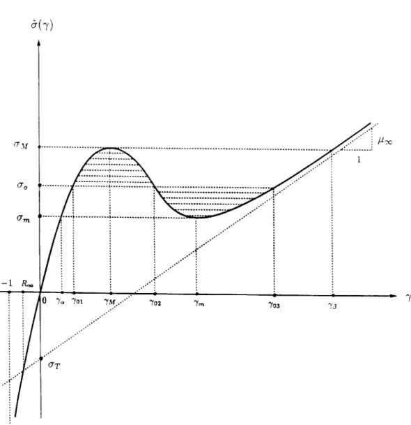
oo, (4.4)

where /tp,(> 0) and 9T are constants. The stress-strain curve therefore consists of three branches, two of which are rising, while the other is declining; it has a single inflection point at the strain-level 7 - 7, and is asymptotic, at large tensile strains, to the straight line 0- p-&y

+

o-T. It is useful for later purposes to note that there are two unique values of

strain R. and P, such that

UooRoo + O-T

=

&(Ro),

&'(P.)

=

po,

where -1

< Ro < Pw < yM;

(4.5)

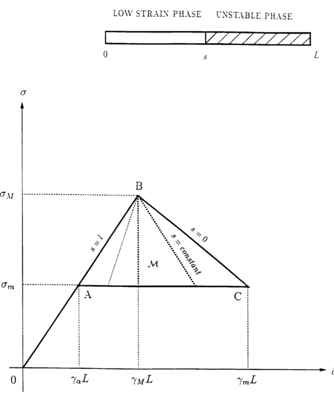
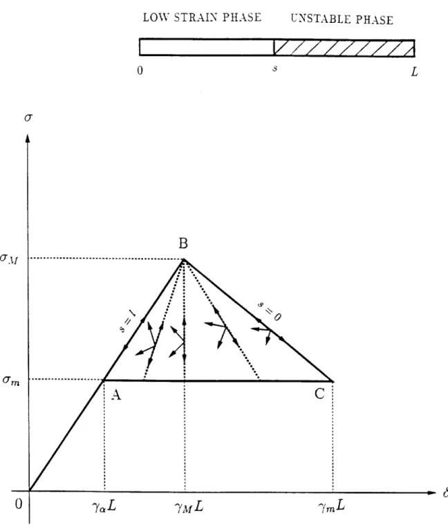
R, is the strain-level at which the asymptote o- = p-Y + 9T intersects the first branch of the stress-strain curve, while P, is the value of strain on the first branch at which the slope equals the slope of this asymptote. Certain other material parameters are defined in the figure. In particular, the Maxwell stress e, is the stress-level for which the two hatched areas of Figure 4.1 are equal.

We shall say that a particle of the bar labeled by x in the reference state is in the low-strain

phase, the "unstable phase" or the high-strain phase at time t during a motion if Y(x, t) lies

in the respective intervals (-1,-YM], (YM7ym) or [7m, oc). At a moving discontinuity x = s(t), the jump conditions (3.3) imply

2 - (>0). (4.6)

A discontinuity is called either a shock wave or a phase boundary according to whether Y

and 7 both lie in the same phase or in distinct phases. The sound speed of the material at a strain - is defined by

c()

=

,

(4.7)

where it is necessary that - in (4.7) not belong to the unstable phase. Let c,, = I1/p.

Let c c(7) stand for the sound speeds on the two sides of a discontinuity. The propagation

speed . of the discontinuity is said to be subsonic if .i

<C

and c , intersonic if c< <

<c

or

c< *.l <C, and supersonic if . 1 >c and c.

We shall speak of a low-strain shock wave and a high-strain shock wave according to whether the strains 7,7 both belong to the low-strain phase or to the high-strain phase. For the material (4.1)-(4.4) considered here, it can be readily seen that all shock waves are

intersonic. Moreover, it follows from (3.7) and (4.1)-(4.4) that the entropy inequality (3.8)

holds at a shock wave if and only if

Low-strain shock:

{

+ if > '1 (4.8)

<

if

A < 0,

High-strain shock:

+<^Y

if- >O0

(4.9)

if < 0.

This implies in particular that a shock wave always moves into the phase whose sound speed is smaller than the speed 1Aj of the shock wave.

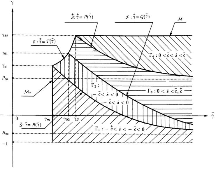
Turning next to phase boundaries, we will show in the next chapter that a phase boundary for which either y or is in the unstable phase cannot arise in the problem to be considered here. Thus suppose that t belongs to the high-strain phase and 7 to the low-strain phase. In the y, y-plane, the set of all pairs (7, 7) for which - is in the high-strain phase, 7 is in the

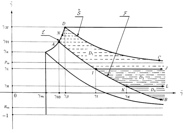
low-strain phase and the right side of (4.6) is non-negative is represented by the union F of the hatched regions in Figure 4.2; it is the region bounded by the lines 7= -1,7= 7M)7= 7m and the curve

&(7)

= &(Y). The region F of the 7,7-plane will play a major role in the analysis that follows in the next chapters. The boundary segment .6 is defined by

E :&(9

=

(')--7

T(7), ym < 'Y < 70,

(4.10)

SOMENNONNNO-where the material parameters y4 and -ym are defined in Figure 4.1. By (4.6), A = 0 at points on E and so this segment represents instantaneously stationary or equilibrium states of the phase boundary. One can verify that T'(-y) > 0 for 7m < y < 70 and that T'(ym)=

0, T'(70) oo; the curve 0

E

therefore rises monotonically as 7 increases. Next, consider the curve

F

which is defined as the set of points

(7,

4

)

at which the driving force

introduced in (3.7) vanishes:

F: f(,)

= 0 -=Q(y), Y 0 , (4.11)

where the material parameter 703 is defined in Figure 4.1. One can verify that Q'(-Y) < 0 and

that Q(-y) - R:,

Q'(7)

- 0 as 7 - oo where P. is the value of strain defined previously in

(4.5). The curve F therefore declines monotonically as y increases as shown in the figure. In view of (3.8), a phase boundary associated with a point on F propagates without dissipation. Since f(j,$) > 0 above F, the entropy inequality indicates that A 0 there; likewise f < 0 and A < 0 below F. Consider next the curves S and S which are defined as the ("sonic")

curves on which the speed A of the phase boundary is equal, respectively, to the sound speeds

c and c:

+S:

(&9

()/9-5

'9

=P(7), 7 > 70,

(4.12)

5:

( ( )-

( ))(

-7)=

'( )

7= R(7), 7

7

-One can

verify

that P'(-), R'(y) < 0

and

that P(-y)

-+

P,,

R(y)

-+

R",

P'(Y), R'(-)

-+

0

as - -> 00 where P, and R, were defined earlier in (4.5). The curves S and S therefore decline monotonically with increasing y as shown in the figure. One can also verify that the three curves 5, S and

F

do not intersect each other; necessarily, the curves

F

and S approach each other asymptotically as 7 -> oo. The region F is thus divided into four subregions 11,

propagate into the high-strain phase at, respectively, intersonic and subsonic speeds; the regions 13 and r4 correspond to phase boundaries which propagate into the low-strain phase at, respectively, subsonic and intersonic speeds. Points on the curves S and S correspond to sonic phase boundaries. For the material (4.1)-(4.4) under consideration, supersonic phase boundaries cannot occur. We note that the figure has been drawn for the case 7Y > P0

though we do not assume this in the analysis.

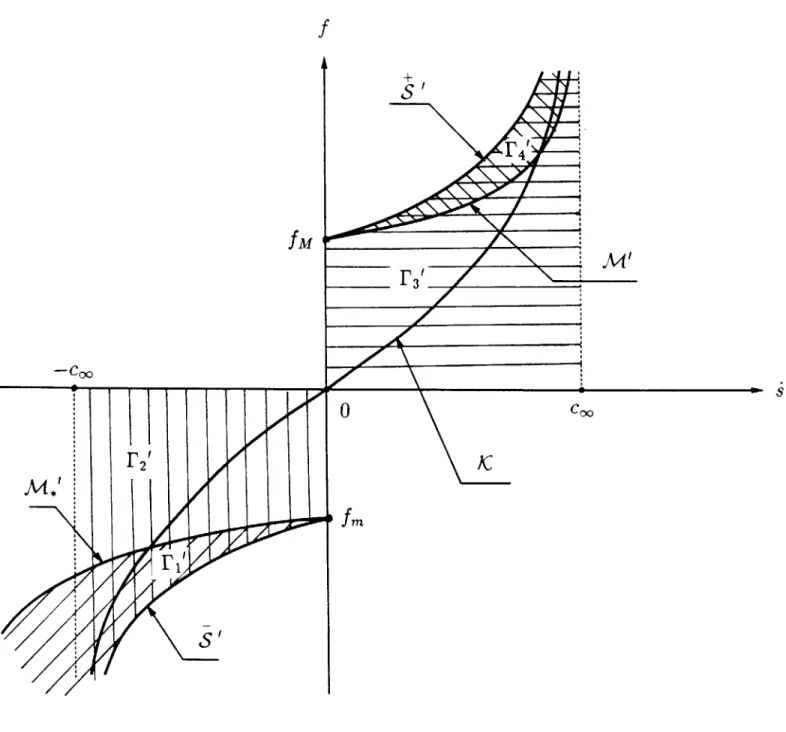
Finally we consider the mapping

(,IY)

(.,f)

defined by (3.7), (3.8) and (4.6). One

can verify that the Jacobian determinant of this mapping vanishes when y, corresponds to a sonic phase boundary, i.e. on the curves S and S. Considering the subsonic and intersonic regions separately, one can map each of the regions F, into the .,

f-plane;

Figure 4.3 shows the images F that result from this mapping. Each of the curves S', S', M' and M' rises

monotonically as . increases. As . -- c.. the curves S' and M' rise without bound; when

-* -cc, the curve S' declines without bound. In Figure 4.3, c,0 = 1ty/p, fm = f( o, Yi)

A +

and

f

m = f (-m,). Note that though this mapping of r from the t, 7-plane to the ., f-plane is not one-to-one, when restricted to the subsonic region F2U F3, it is one-to-one.

&N

(7 ... ... _... ... ... ... ... ... ... 010 ... ... 4 --- ... ... ... ... ... ... .... --- ... ... .... R. 7, 'Yol 702 ₇₀₃ ' 3 (7T

'Y03 70 + c< S < - c< 0 .... .... ... .. . . . .... ... .... .... ... ... ... ... .... .... ... .... . ... .... ... ... . .. ... ... ... .... ... ... ... ... . .... .... .. ... z 0 7m s: ROO ... ---Roo - I

Figure 4.2. The regions ri in the

+)-plane.

... Y= T(-O ... .... c c r4 0 <+< < ---... _... 4 ... r2 + r3 0 < <c c c< q < 0 + c < q < 0

P(-Y)

Q(10

7cf POO

f

fM - coo

SI

4 POW _M' A~~~'*\

z.-~

0

coo

AZ

I fm

Figure 4.3. Admissible images of Pi in (s. f)-plane.

S

0/ 00000

elo

00e

1100or

140"

-I

Chapter 5

The Riemann Problem: Construction

of Solutions

5.1

Formulation

We now formulate the Riemann problem for the field equations and jump conditions

(3.2)-(3.3). We seek weak solutions of the differential equations (3.2) on the upper half of the x, t-plane that satisfy the following initial conditions:

fL7,VL,

-oo <

X

<

O,

(X, 0), v(x, 0) =

(5.1)

7R, VR, 0 < X < oo,

where -L, 7R, VL and VR are given constants with -Y > -1 and yI > -1.

Since the initial value problem described above is invariant under the scale change t--+kt, X-+kx, we restrict attention to solutions that have this property as well. Where such solutions exist, they must have the form y(x,t) = ((), v(x,t) = O( ) where = x/t. It then follows

from (3.2) that for such solutions, either -y and v are both constant, or they are the wave

fans which are given by

=

p(,

(5.2)

A

The left side of (5.2) must necessarily be non-negative for any ^ that satisfies (5.2). Thus for the material (4.1)-(4.4) wave fans can occur only if

-

takes values in either the low-strain phase or the high-low-strain phase. We shall speak of a low-low-strain fan or a high-low-strain fan according to whether belongs to the low-strain phase or the high-strain phase respectively. In view of (4.1)-(4.4), it follows that (5.2) defines a unique function ^(') = Y(L)( ) for -o < < oo, such that -y(L) E (-1,YM; Y(L) describes the strain field in a low-strain fan.

Similarly (5.2) can be uniquely solved for a function

^(

)

= 7

(H)( ) for -c. < < c.,

such that 7(H) E -Y_m

,

10); 7 (H) describes the strain field in a high-strain fan. Thus (5.2),

(5.3) lead to the two wave fans

)= ( () =v()( ), i = L H, where (5.4)

()

-

v(i)((o))

=

±i]

c(7-)d-y,

i = L, H,

(5.5)

and , describes an arbitrary ray x/t = , within the fan; necessarily (, must lie in the interval (-oo, oo) for a low-strain fan and in the interval (-c,, c.) for a high-strain fan. The positive and negative signs are taken in the right side of (5.5) according to whether the wave fan occurs in the first quadrant or second quadrant of the x, t-plane, respectively.

Consider two rays x = Ct and x = ct with C < c in the (x, t)-plane between which the

field is a fan. Let 7= 7t(Ct+,

t),

V= v(Ct+, t), t= Y(ct-, t), V= v(ct-, t) denote the limiting

values from within the fan of strain and particle velocity at these rays. It follows from (4.7) and (5.2) that

C= icy), c = ±c(y), (5.6)

and from (5.3) that

where the positive and negative signs are taken according to whether the fan occurs in the first or second quadrant of the x, t-plane, respectively. Equation (5.7) is the analog for a fan of the kinematic jump condition for a discontinuity in (3.3). Since the field within the fan is smooth, the entropy inequality is trivially satisfied at points within it. For the material

(4.1)-(4.4), it follows from (5.2) that necessarily

Low-strain fan:

{

if fan is in first quadrant,

(5.8)

7>-f if fan is in second quadrant,

High-strain fan: 7>-Y if fan is in first quadrant, (5.9)

<Y if fan is in second quadrant.

Equations (5.8)-(5.9) are the analog for fans of equations (4.8)-(4.9) for shocks. Conversely, given numbers (7, ), (7, v) which conform to (5.7)-(5.9), one can construct a unique fan

between the rays x =t and x = ct where c is given by (5.6).

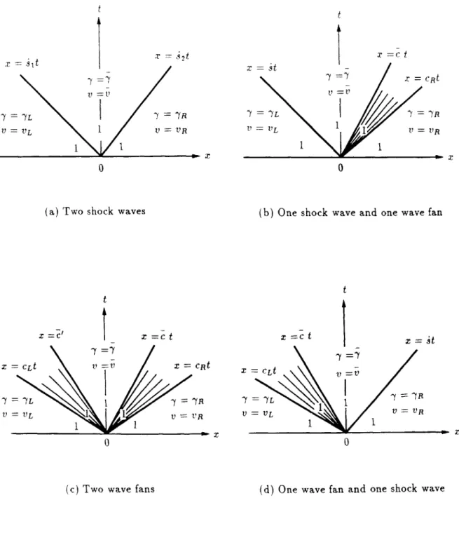
The general scale-invariant solution to the Riemann problem has the form shown in Figure 5.1: between any two rays x = .it and x = i+it the fields ,v are either constants or fans; the rays themselves may or may not correspond to discontinuities. If x = .,t is a

discontinuity, the jump conditions (3.3) must be satisfied across it so that

(7i

-

71-1)

=

-(vi

-

v _ ),

where (yi, vi) and (yi_1, v_1) are the limiting values of strain and particle velocity on the right and left respectively of this discontinuity. Let

fi

= f(-yi1,y) with

f

defined by (3.7) stand for the driving force on this discontinuity; the entropy inequality (3.8) then requires that

fi

i ;> 0.

(5.11)

An admissible solution of the Riemann problem is a pair 7(x, t), v(x, t) of the form just described with (5.10)-(5.11) enforced at all discontinuities.

5.2

The Structure of Admissible Solutions to the

Rie-mann Problem

The initial data in (5.1) is said to be metastable if neither of the initial strains (L, YR belong to the unstable phase. Before constructing explicit global solutions to the Riemann problem, it is helpful to establish some general results pertaining to the permissible solution forms that are consistent with the entropy inequality.

Let (-, v) be an admissible solution of the Riemann problem with metastable initial data.

(i) The strain y(x, t) does not belong to the unstable phase at any point (x, ) in

the upper-half plane.

This result implies that if the initial data does not involve the unstable phase, then at no later time does the solution involve the unstable phase. We prove this claim by contradiction. Suppose that this proposition is false. Since unstable phase fans and shocks do not exist, there must necessarily be two phase boundaries in the (x, t)-plane, say x = .kt and x = k+1t

with .k < k+1, such that the state between them is constant with the associated strain yk in

the unstable phase and with neither of the strains -f_1 = y( t-, t) and 7yk+l = 7(hk+1t+,t) in the unstable phase. From (3.7) and (4.1)-(4.4) one sees that the driving force on the discontinuity x = hkt is positive; the entropy inequality (5.11) thus implies that .k > 0. Similarly the driving force on x = k+1t must be negative and so hk+1 < 0. Thus hk ;> hk+1 which is a contradiction. This establishes the proposition.

The next six propositions are concerned with the possibility of having shock waves, phase boundaries and wave fans adjacent to each other. When addressing fans, it is sufficient for our purposes to restrict attention to fans which do not terminate on discontinuities. Thus in the propositions that follow, if x = skt and x = .k+1t are two rays in the (x, t)-plane between

which the field is a fan, these two rays will be assumed not to be discontinuities. Features of fans which do terminate at discontinuities can be deduced from the following results by

suitable limiting arguments.

Let (-y, v) be an admissible solution of the Riemann problem with metastable initial data.

(ii)

Let x = t, x = .k+1 t, x = .k+2t and x = k+, be

four

rays in the same

quadrant of the (x,t)-plane. If the

field

in the interior wedge jk+ 1t < x < .k+ 2t

is constant, then the field in the other two wedges cannot both be fans.

(iii) Let x =kt and x = .k+lt be two rays in the same quadrant of the

(x,t)-plane between which the field is constant. Then these two rays cannot both be shock waves.

(iv) Let x = kt and x = k+1t be two rays in the same quadrant of the (x, t)-plane

between which the field is constant. Then these two rays cannot both be phase boundaries.

(v) Let x = kt, x = k+1t and x = k+2t be three rays in the same quadrant of

the (x,t)-plane. Suppose that the field between any two of these rays is a

fan.

Then the third ray cannot be a shock.

(vi) Let x = kt, x = .k+lt and x = k+2t be three rays in the same quadrant of the (x, t)-plane. Suppose that the field between the two slowest rays is a

fan.

Then the remaining ray cannot be a phase boundary. (The converse case is possible: if the field between the two fastest rays is a fan the remaining ray may be a phase boundary.)

(vii) Let x = .kt and x = Ak+lt be two rays in the same quadrant of the (x, t)-plane. If the slower ray is a shock, then the faster ray cannot be a phase boundary.

(The converse case is possible: if the faster ray is a shock, the slower ray may be a phase boundary.)

The first three of these propositions state that two wave fans, two shock waves and two phase boundaries cannot be adjacent to each other. The next one states that a fan and a shock cannot be adjacent to each other. On the other hand according to proposition (vi), a fan and a phase boundary may be adjacent to each other provided the phase boundary is subsonic. Similarly a shock and a phase boundary may be adjacent to each other provided the phase boundary travels more slowly than the shock.

It is clearly sufficient to prove these results in any one quadrant of the upper-half of the (x, t)-plane and so we shall consider only the first quadrant. Thus in each of these propositions we have 0 < 5

k < 8k+1 < sk+2 < 3

k+3-To prove proposition (ii), suppose that it is false so that the field in .kt < X < k+1t

and k+2t < X < k+3t are fans while the field is constant in the intermediate wedge. It is not possible that one of these fans is a low-strain fan while the other is a high-strain fan, since such fans belong to different phases and so must necessarily be separated by a phase boundary. For two fans of the same type, (5.2) directly shows that they must in fact be smoothly connected to each other to become a single fan with .k+i = .k+2. This contradicts

the assumption that k+1 < k+2. The assertion (ii) is thus proved.

We now turn to the proof of proposition (iii). Suppose that the proposition is false so that x = .kt and

x

= k+1 t are both shocks and the field between them is constant. Note first that a low-strain shock cannot be adjacent to a high-strain shock, since they must be separated by a phase boundary. Suppose that both x = .kt and x = k+1t are low-strain

vk-l k-1 i

J

X =

.kt-7(X, t), V(X, t) =kk, Vk, 4t < X < 4k+1t,

(5.12)

Yk+l, Vk+1, X = 4k+1t+

where 7k1, -Yk and 7k+1 are distinct and all three belong to (-1,yMl. According to (5.11), the driving forces acting on these two shock waves must be non-negative. With the help of

(3.7) one finds that this implies that N-1 < -k < -/k+1. Since 6'(y) > 0 and &"(-)

<

0 on

(-1,7M), this, together with the fact that -1 < 7k_1 < -k < 7k+1 7M, implies that

&(Yk+1) -&(7k) K &(7k) -{(-1) _(5.13)

Jk+1 - k 7k - ^/k-1

Equations (5.10) and (5.13) then yield 4, > 4+1 which is a contradiction. In a similar way, we can prove that two high-strain shocks cannot be adjacent to each other. This proves proposition (iii).

Propositions (iv) and (vii) may be established by arguments that are very similar to the above.

Next we turn to the proof of proposition (v). Suppose that it is false. Note first that a low-strain shock cannot be adjacent to a high-strain fan (or vice versa) since they must be separated by a phase boundary. Suppose that x = 4t is a low-strain shock and that the

field between the rays x = 4+ 1t and X = 4+ 2t is a low-strain fan:

k-1, Vk-1, X =

kt-N ,Vk, kt < X < k+1t,

7(x,

t), v(xt)

=

(5.14)

7 (L)(X/t), V(L)(Xlt), 4k+1t <_ X <_ 4+2t,

^/k+2,1k+2, X = 4+2t+,

where 7_Y1,7Y, and 7k+2 all lie in the strain phase and -y(L) is the strain field in a low-strain fan given by (5.4). For the material (4.1)-(4.4), equation (5.2) and the fact that

Sk+1 < sk+2 implies that 7k > 7k+2. Next, the entropy inequality (5.11) requires the driving

force f(Yk_1,Yk) at x = kt to be non-negative; by (3.7), this implies that Yk-1 < 74. Since d'(-) > 0 and 4"(-) < 0 on [7k_1, yk, this, together with the fact that -1 < 7k-1 < 7k 7M implies that

&,(7k) &(7k) - 6Yk-1)

(5.15)

7 - ^A-1

Equations (4.7), (5.10) now yield > 4+1 which is a contradiction.

The remaining cases where x = 4+2t is a low-strain shock and the field between the rays

x = 4t and = k+1t is a low-strain fan, and when the shock and fan are both high-strain ones, can be treated similarly. This establishes proposition (v).

The proof on proposition (vi) is entirely analogous.

The preceding results imply that the form of admissible solutions to the Riemann problem with metastable initial data is in fact much simpler than that described in Figure 5.1. Note that the results (iii)-(vii) depend critically on the entropy inequality (5.11).

t

x

=

t

X ₂

_t

_4.

*... X=SN-it SNt

0

= 7L, V = VL

Figure 5.1.

1

= 7RV V = yR

General form of solutions to the

Riemann problem.

Chapter 6

Explicit Solutions to the Riemann

Problem

The results established in the preceding chapter allow one to determine all admissible solu-tions to the Riemann problem in the case of metastable initial data. From here on we shall consider only the special Riemann problem in which the initial strains 7L and YR are both

in the low-strain phase, and -YR is smaller than 7L:

-YL E ( -L l, ^M] G3 (-1,7M], 7R < tL-

(61

At the initial instant, the entire bar is in the low-strain phase. At a later instant, a particle of the bar may or may not change its phase. It is convenient in the following analysis to consider these two cases separately.

6.1

Solutions Involving No Phase Change

In this case, the solution does not involve any phase boundaries. In view of the first propo-sition in Section 5.2, neither does it involve the unstable phase at any time t > 0. Next, in view of propositions (ii), (iii) and (v), the solution -, v can only involve a single low-strain shock wave or a single low-strain fan in each quadrant of the upper half of the x, t-plane.

(i(a)) Solution with two shock waves. Figure 6.1(a). Consider a solution having the form

shown in Figure 6.1(a):

7L, VL, y,v = y,V,

7fR,

VR, -00 < x

< ilt,

.st < X < 2t, 2t < X < OCoi

in which 7,i, i and 2 are to be found such that ' E

(-1,7M]

and .1 < 0 < 2.

The jump conditions (5.10) and the entropy inequality (5.11) at each of the two shock waves require that

-(yR - V) = A2( ---(V - VL) = -S2 = _ , po_ -7) pC~Y - xL)

The inequalities in (6.1), (6.3), (6.4), together with the requirement that 7 be in the low-strain phase, imply that

-1<

<YR

(6.5)

Combining (6.3)-(6.4) yields

VR - VL = H(),

where H(-y) is defined on (-1,7R] by

H(7')

- [ (-M) - 6(-Y)(7R - /p

-

v'a~~-y

-It can be verified that H(-y) increases monotonically on (-1,7R] from the value -oo at

S-= -1 to the value HR = H(-YR) at -y = -R. Thus if the initial data is such that -oo <

(6.2)

71R > Y, (6.3)

Y<

7L-

(6-4)

(6.6)

yR - VL < HR, there is a unique root y of (6.6) in the range -1 < I < -YR(< -M). The remaining unknowns s, . and '2 are then given immediately by (6.3) and (6.4).

Thus, there exists a unique admissible solution of the form (6.2) corresponding to Figure

6.1(a) if and only if the given initial data (5.1), (6.1) is such that -oo

< VR - VL< HR.

(i(b)) Solution with a shock wave and a wave fan. Figure 6.1(b). Consider next a solution

of the form shown in Figure 6.1(b):

't rVL,

-00 < x < R7,

7,1 VI < x <ct,

I, =(6.8)

'(x/t), i(x/t), Ct < X < CRt,

, RVR, CRt <X 00,

where , s ., c and CR are to be determined such that (-1,yM] 1 and < K 0 < C <

CR-The functions -(x/t) and i(x/t) are the strain and velocity fields pertaining to a low-strain

fan and are given by (5.4)-(5.5).

At the shock wave x = t, the jump conditions (5.10) and the entropy inequality (5.11) must hold:

(6.9)

tu net t the fan, a y i 6( , < 7L.

Turning next to the fan, and by using

(5.6)-(5.8),

one finds

(V-

'R)

J

c()dy,

'YR

Equations (6.9)-(6.10) may now

VR - VL

H(m)

where

CR = c(YR), c = c(l), Y > .YR.

(6.10)

be combined to yield