Discrete time quantum walks : from synthetic gauge fields to spontaneous equilibration

(1)

HAL Id: tel-01230891

https://tel.archives-ouvertes.fr/tel-01230891

Submitted on 19 Nov 2015

HAL is a multi-disciplinary open access archive for the deposit and dissemination of sci-entific research documents, whether they are pub-lished or not. The documents may come from teaching and research institutions in France or abroad, or from public or private research centers.

L’archive ouverte pluridisciplinaire HAL, est destinée au dépôt et à la diffusion de documents scientifiques de niveau recherche, publiés ou non, émanant des établissements d’enseignement et de recherche français ou étrangers, des laboratoires publics ou privés.

Discrete time quantum walks : from synthetic gauge

fields to spontaneous equilibration

Giuseppe Di Molfetta

To cite this version:

Giuseppe Di Molfetta. Discrete time quantum walks : from synthetic gauge fields to spontaneous equilibration. Physics [physics]. Université Pierre et Marie Curie - Paris VI, 2015. English. �NNT : 2015PA066220�. �tel-01230891�

(2)

Université Pierre et Marie Curie

École Doctorale Physique en Île de France (ED 564)

Laboratoire d’Étude du Rayonnement et de la Matière en Astrophysique et Atmosphères (LERMA)

Discrete time quantum walks:

from synthetic gauge fields to spontaneous equilibration

Par Di Molfetta Giuseppe

Thèse de Doctorat en Physique Théorique

Directeur: Fabrice Debbasch (LERMA - UPMC) Co-directeur : Marc Brachet (LPS ENS, CNRS)

Présentée et soutenue publiquement le 28/07/2015

à l’Université Pierre et Marie Curie, devant un jury composé de :

M. Jean-Michel Raimond Professeur Examinateur

M. Dieter Meschede Professor Rapporteur

M. Pablo Arrighi Professor Rapporteur

M. Yutaka Shikano Professeur Examinateur

M. Fabrice Debbasch Maître de Conférence Directeur de thèse M. Marc Brachet Directeur de Recherche (Invité) Co-directeur de thèse

Except where otherwise noted, this work is licensed under http://creativecommons.org/licenses/by-nc-nd/3.0/

(3)

(4)

Remerciements

J’ai commencé ma thèse en septembre 2012 au Laboratoire d’Études du Rayonnement et de la Matière en Astrophysique et Atmosphères (LERMA) de l’Observatoire de Paris, dont je tiens à remercier l’ex-directeur Michel PÉRAULT et l’actuel l’ex-directeur Darek LIS pour leur accueil au sein de leur unité. Je remercie également Maryvonne GERIN pour m’avoir accueilli dans son èquipe du LRA à l’Ecole Nor-male Supérieure où j’ai passé mes deux premières années de these, et Chantal STEHLE pour avoir fait de même à Jussieu pendant ma dernière année.

Cette thèse a été dirigée par Fabrice DEBBASCH, que j’ai rencontré pendant mon premier stage de M1 à l’Université Pierre Marie Curie. Avec lui, j’ai découvert le sujet de ce doctorat et j’ai échangé sur une infinité de sujets scientifique. Je le remercie pour la confiance et le soutien dont il a fait preuve pen-dant tout mon travail, jusqu’aux derniers jours de rédaction du manuscrit. Ce qu’il ma donné de plus précieux, c’est son grand enthousiasme pour la science, la recherche et la découverte, que je garderai dans mon futur professionnel. Je voudrais également remercier Marc-Etienne BRACHET pour m’avoir co-encadré pendant ces trois ans. Notamment, je lui suis reconnaissant pour sa patience, son expertise scientifique et la transmission d’une partie de son énorme connaissance. À lui va aussi ma gratitude sa profonde humanité.

Je voudrais également remercier Martine BEN AMAR pour m’avoir accueilli dans le Master de Physique des systèmes complexes et Jean-Bernard ZUBER pour sa disponibilité pendant mes premiers mois de permanence à Paris. J’exprime ma plus profonde reconnaissance à Pablo ARRIGHI et Dieter MESCHEDE qui m’ont fait l’honneur d’accepter d’être rapporteurs de la prèsente thèse (thank you Prof. P. ARRIGHI and Prof. D. MESCHEDE to have accepted to be the examiners of this thesis). J’associe à ces remer-ciements les autres membres de jury: Jean-Michel RAIMOND et Yutaka SHIKANO. En particulier je remercie J.-M. RAIMOND pour l’intérêt qu’il a montré envers les résultats que j’ai obtenu lors de mon premier stage.

Je suis aussi reconnaissant envers Y. SHIKANO pour son accueil au sein de son unité à Okazaki. Mon séjour au Japon, qui a été la plus belle et intense expérience professionnelle pendant mon doctorat, aurait été très difficile sans la disponibilité et la sympathie de Naoko KONDO, Mayuko KATO et tous les autres membres du IMS. Je remercie parement Beatrice GUIBAL du LERMA pour avoir géré toutes mes questions administratives. Pendant ces trois années de travail, j’ai eu l’occasion de profiter de la grande expertise de Giorgio KRSTULOVIC, Stéphan FAUVE, Fabio SCIARRINO, Stéphane ATTAL, Carlo DI FRANCO, Christopher CEDZICH, Fumiaki MATSUOKA, Yu-Xiang ZHANG et Tatsuaki WADA. Je les remercie pour leurs nombreux et précieux conseils. Je remercie aussi, pour leur esprit convivial et la patience d’avoir partagé le bureau avec moi, Marco PADOVANI, Lionel de SA et Uddhab CHAULAGAIN. En particulier Pablo ARNAULT pour son humilité et son vrai enthousiasme pour la physique.

Merci aussi à mes frères de l’école Nam Anh qui m’ont aidé à tracer ma route, et à tous les amis qui m’ont soutenu et fait sourire sur ce chemin parfois difficile.

Une remerciement spécial va à ma famille, notamment ma mère qui n’a jamais arrêté de croire en moi et de m’encourager.

Je dédie cette thèse à Vera qui m’a enseigné à écouter avec amour.

Caminante, son tus huellas el camino y nada mas; Caminante, no hay camino, se hace camino al andar. (A.M.)

(5)

(6)

spontaneous equilibration.

ABSTRACT

Keywords: Discrete Time Quantum Walks, Quantum Simulations, Synthetic Gauge Fields Quantum Decoherence, Quantum Gauge Lattice, Thermalization.

Problems too demanding for classical computers can be approached promisingly with quantum simulators, which operate using one controllable quantum system in order to inves-tigate the behavior and properties of a less accessible one. Over the past few years, significant progress has been made in a number of experimental and theoretical fields. Quantum Walks (QWs) are simple and sophisticated discrete space and time dynamical systems and it has been shown that in the continuous limit different emergent quantum fields can be simulated. In this thesis we will draw on QWs to further explore various areas of interest in Physics. More specif-ically our analysis will branch out into three main directions: (i) the connection between QWs and quantum field theory, with particular attention to bridging the quantum coin of QWs with the geometrical properties of gauge field theories; (ii) the study of QWs’ classical limit and of the transient semi-classical dynamics, especially in relation with field theories; (iii) the spon-taneous equilibration and thermalization in some nonlinear QWs-like models. Every step of this thesis will be validated by specific analytical results and numerical implementations.

(7)

(8)

synthèse à l’équilibration spontanée

RÉSUMÉ

Les simulateurs quantiques, qui utilisent un système quantique contrôlable pour étudier le comportement et les propriétés d’un autre système quantique, moins accessible, sont une ressource prometteuse. Dans les dernières années, des progrès significatifs ont été faits dans de nombreux domaines expérimentaux et théoriques. Les marches quantiques à temps dis-cret sont des systèmes simples et sophistiqués. En particulier, il a été montré qu’à la limite continue, ces marches peuvent simuler certaines théories de champs. Dans ce travail de thèse, lesdites marches sont utilisées pour explorer certains sujets d’intérêt physique, qui s’articulent autour de trois axes : (i) la connexion entre les propriétés géométriques de la marche et celles de divers champs de jauge ; (ii) la limite classique et la limite quasi-quantique, en relation surtout avec les théories de champs ; (iii) l’équilibration spontanée pour certains modèles non linéaires de marches quantiques. Chaque résultat est appuyé par une étude numérique et an-alytique.

Mots-clés: Marches quantiques à temps discret, Simulation quantique, Champs de jauge de synthèse, Décohérence quantique, Théories de jauge sur réseau, Thermalisation.

(9)

(10)

List of Figures

1.1 Spread of probability density of a Hadamard walk on n grid points with

asymmet-ric initial state ™0=Pm√0,m(cL|bLi + ei ¡cR|bRi) T where (i) cL= 1,cR= 1,¡ = 0

or (ii) cL= 1,cR= °1,¡ = 0 and symmetric initial state cL= 1,cR= 1,¡ = º/2. The

spatial component is given by √0=Pm±0,m . . . 14

1.2 Square root of variance of a Hadamard Walk with symmetric initial state and lo-calized position in the origin. The slope is (1 °p1

2)

1/2_. _{. . . 15}

1.3 Spread of probability density of the DTQW with symmetric initial state and dif-ferent values of µ, for Æ = °º/2, ª = º/2 and ≥ = º/2. . . . 15

1.4 Value of Kµfor a given µ. . . . 16

1.5 Feynman’s Checkerboard representation in the discrete space time lattice (x, t). . 18

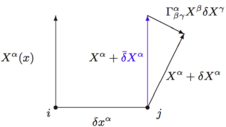
2.1 Distortion in a vector field in the transport from a point i to a point j of the curved spacetime.. . . 42

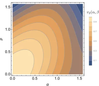
3.1 Variation of entropy of measurement (or entanglement) (Sr)j VS time for

differ-ent values of µ. Inside the figure: the variation of differ-entropy VS µ for a given number of steps. . . 74

4.1 Classical Galton Board.. . . 106

4.2 (Left) The optical ring cavity for the implementation of the Optical Galton Board. The EOMs are the electro-optical modulators and the BS is the beam splitter. The solid gray rectangle is the partially reflecting mirror serving as input and output port and the black ones are the fully reflecting mirror of the cavity.(Adapted from Knight et al. [10]) (Right) On the top the probability distribution of a classical Galton board, and on the bottom the density profile of frequencies in the wave-mechanical case within the Landau-Zener crossings. ©1is a control parameter

(15)

(16)

I

NTRODUCTION

Quantum simulation has recently established itself as an area of study in quantum physics that merges fundamental and applied questions. Such an interaction results in a more opera-tional understanding of some aspects of quantum mechanics in terms of nature description. The idea to simulate the dynamics of a quantum system by a quantum device was first intro-duced by Richard Feynman in a seminal article in 1982 [19] and developed in different frame-works, from quantum optics to condensed matter physics.

A way to describe quantum systems and their dynamics within a computational perspective is given by the large class of Quantum Cellular Automata (QCA), that is a grid of quantum au-tonomous systems, interacting through local rules [44,37,8,7,38]. Over the last years, many definitions and models of QCA have been proposed. For instance, Schumacher and Werner [37] proposed a class of reversible QCA, where the evolution of the QCA is given by local uni-tary operations that act on the neighborhood of a given cell, and it is further updated by a single cell unitary operation. This is in accordance with the expected microscopic fully quan-tum dynamics. However in recent years an agreement has been achieved and many definitions have been proven to be equivalent by Arrighi and Grattage [6].

This class of quantum systems displays a wide range of complex phenomena and it has been extensively used for the comprehension of Quantum Field Theory (QFT). Bialynicki-Birula [9] first underlines the connection between QCA and QFT. Then Meyer [29] showed that QCA mostly correspond to lattice gas models and are closely related to the Dirac equation; in addition to this, again Meyer and Shakeel [30], have recently proved that QCA with no particle interpretation exist and that they propagate information.

Quantum Walks (QWs) are a special case of reversible QCA , but in the sigle particle sector. Differently from QCA, they describe the unitary dynamics of one quantum particle. They have been introduced independently by Grossing and Zeilinger [22] and Y. Aharonov et al. [3] and then extended systematically on graphs by D. Aharonov et al. [2]. QWs have been, later, fully mathematically examined by Konno [27].

Quite surprisingly, this simple one-particle quantum automaton is an excellent tool for modeling a large spectrum of physical phenomena and it is interesting both for fundamen-tal quantum physics and for physical applications. Already in the formal introduction by Y. Aharonov, QWs appear as models of coherent quantum transport. Therefore it is not aston-ishing that Feynman and Hibbs [18] provided a model of QCA, the "Feynman Checkerboard", resembling QW, as path discretization of the Dirac propagator.

Let us remark that all these historical landmarks concern the so-called Discrete-Time Quan-tum Walk (DTQW), that is an automaton living in discrete time and discrete space. Whilst a continuous-time version of QW (CTQW) - living in continuous time and discrete space - has been introduced independently in the literature, we will not deal with it in the present work. Just let us keep in mind that, even though both models are mathematically defined in a

(17)

differ-2 INTRODUCTION

in the continuous limit.

Nowadays QWs can be realized experimentally with a large spectrum of physical objects and setups. A first natural way to physically implement a QW is in optical networks. For in-stance, Knight et al. [26] realized experimentally the first optical implementation of a QW in an optical ring cavity, as a modified experimental setup of the optical linear quincunx described by Bouwmeester et al. [10], the Optical Galton Board.

A second way to implement QWs is the Nuclear Magnetic Resonance (NMR), proposed by Ryan et al. [33] for a DTQW, subsequent to the work of Du et al. [15]. This method consists in manipulating and coupling spin orientations, in constituting quantum logic gates and in performing unitary operations on the nuclei quantum state in the magnetic field.

Other possible implementations can be realized in Quantum Electrodynamics (QED). In effect, the physical scheme proposed by Y. Aharonov in its seminal paper [3] has inspired Agar-wal and Pathak [1] to realize a DTQW in this framework. They implemented it by injecting a single Rydberg atom into an optical cavity and by driving it by a strong external field. The ef-fective Hamiltonian introduced in their article reproduces perfectly the Aharonov’s scheme. A more recent implementation of QW in cavity QED is due to Sanders et al. [34].

Other techniques range from quantum optics (Zhang et al. [45], [46]), to ion traps (Travaglione and Milburn [43]), and to neutral atom traps (Chandrashekar [12],Eckert et al. [17], Dür et al. [16]). In particular, quite useful for the implementation of QWs on cycle is the interacting quantum dots architecture presented by Solenov and Fedichkin [40] in a solid state framework. Recent developments, however, have shown an increasing interest for two or more corre-lated QWs, due to the large class of emergent quantum phenomena (Peruzzo et al. [32], San-soni et al. [35], Schreiber et al. [36] and more recently Defienne et al. [14]). However, this thesis is dedicated to the study of the single-particle dynamics and we will not take into account multi-particle systems.

As for the physical implementations, the potential applications of QWs are too numerous to be listed here. They spread from search algorithms [13] and graph isomorphism [4, 21] to modeling and simulating quantum dynamics [36] and classical system [41]. We can redi-rect the reader to Lovett et al. [28] for an introductory review on the quantum walk algorithm. Concerning modeling quantum dynamics we can recall some remarkable applications in con-densed matter. For instance, in topological insulators realization [25,24], for spintronic appli-cations [23], and for quantum transport on 2-dimensional layer, as in graphene-like materials [20].

This thesis is specifically devoted to only one of the various DTQWs’ applications: quan-tum simulation of quanquan-tum systems dynamics. In particular, let us remind the reader that, rather than a monograph, this manuscript appears as a collection of our main publications with an accurate introductory section to each of them. All our works deal with QWs propagat-ing in one spatial dimension.

The thesis is organized in three main parts and four chapters. In the first part, the Chapter (1) is devoted to introduce DTQWs and report their main features, largely explored in the cent literature. In particular, we present the method to perform the continuous limit and its

(18)

re-lated sufficient conditions. Moreover, we formally prove that not all families of homogeneous DTQWs (HDTQWs) admit such conditions. In Chapter (2), we extend the same analysis to the inhomogeneous DTQWs (IDTQWs) and we introduce the idea of synthetic gauge field. Above all, we prove that some special families of IDTQWs mimic the propagation in curved (1 + 1)-spacetime of a Dirac fermion, coupled to a gauge electric potential. Let us recall that similar results have been recently obtained by our group in a (1+2) spacetime dimension (Arnault and Debbasch [5]). We conclude the first part with Chapter (3), introducing a randomized version of the IDTQW. We analytically provide detailed calculations demonstrating the loss of coher-ence and the emergent classical diffusive behavior of the walk.

In the second part and last chapter, Chapter (4), our analysis concerns the very new prob-lem of equilibration in QWs. Generally, equilibration is the process through which a system, under a given dynamics, reaches a steady state. By thermalization we mean that this steady state can be interpreted as a thermal state at a given temperature.

Thermalization is observed typically in nonlinear systems, but all QWs describe the motion of a single particle and are linear by definition. Moreover nonlinear QW-like implementations have been considered in different contexts. In the context of optics, the so-called Optical Gal-ton Boards (OGB) [11] have been generalized to include nonlinear Kerr effects by Navarrete-Benlloch et al. [31] or in Shikano et al. [39], who proposed a DTQW with feed-forward quan-tum coin displaying high nonlinearities. In those models very complex and rich behaviors have been observed. The aim of this last chapter, and our main contribution, is to observe and characterize thermalization phenomena in a spatially-periodic version of the Nonlinear OGB.

(19)

4 INTRODUCTION

Bibliography

[1] G. S. Agarwal and P. K. Pathak. Quantum random walk of the field in an externally driven cavity.

Physical Review A, 72(3):033815, 2005.

[2] D. Aharonov, A. Ambainis, J. Kempe, and U. Vazirani. Quantum walks on graphs. In Proceedings of

the thirty-third annual ACM symposium on Theory of computing, pages 50–59. ACM, 2001.

[3] Y. Aharonov, L. Davidovich, and N. Zagury. Quantum random walks. Phys. Rev. A, 48:1687, 1993. [4] A. Ambainis. Quantum walks and their algorithmic applications. International Journal of

Quan-tum Information, 1(04):507–518, 2003.

[5] P. Arnault and F. Debbasch. Landau levels for discrete-time quantum walks in artificial magnetic fields. arXiv preprint, 1412.4337, 2014.

[6] P. Arrighi and J. Grattage. Partitioned quantum cellular automata are intrinsically universal.

Nat-ural Computing, 11:13, 2012.

[7] P. Arrighi and J. Grattage. Partitioned quantum cellular automata are intrinsically universal.

Nat-ural Computing, 11(1):13–22, 2012.

[8] P. Arrighi, V. Nesme, and R. Werner. One-dimensional quantum cellular automata over finite, unbounded configurations. In Language and Automata Theory and Applications, pages 64–75. Springer, 2008.

[9] I. Bialynicki-Birula. Weyl, dirac, and maxwell equations on a lattice as unitary cellular automata.

Physical Review D, 49(12):6920, 1994.

[10] D. Bouwmeester, I. Marzoli, G. P. Karman, W. Schleich, and J. Woerdman. Optical galton board.

Physical Review A, 61(1):013410, 1999.

[11] D. Bouwmeester, I. Marzoli, G. P. Karman, W. Schleich, and J. P. Woerdman. Optical Galton board.

Phys. Rev. A, 61:013410, Dec 1999. doi: 10.1103/PhysRevA.61.013410. URLhttp://link.aps. org/doi/10.1103/PhysRevA.61.013410.

[12] C. Chandrashekar. Implementing the one-dimensional quantum (hadamard) walk using a bose-einstein condensate. Physical Review A, 74(3):032307, 2006.

[13] A. M. Childs, R. Cleve, E. Deotto, E. Farhi, S. Gutmann, and D. A. Spielman. Exponential algorithmic speedup by a quantum walk. In Proceedings of the thirty-fifth annual ACM symposium on Theory

of computing, pages 59–68. ACM, 2003.

[14] H. Defienne, M. Barbieri, I. A. Walmsley, B. J. Smith, and S. Gigan. Control of two-photon quantum walk in a complex multimode system by wavefront shaping. arXiv preprint arXiv:1504.03178, 2015. [15] J. Du, H. Li, X. Xu, M. Shi, J. Wu, X. Zhou, and R. Han. Experimental implementation of the

quan-tum random-walk algorithm. Physical Review A, 67(4):042316, 2003.

[16] W. Dür, R. Raussendorf, V. M. Kendon, and H.-J. Briegel. Quantum walks in optical lattices. Physical

Review A, 66(5):052319, 2002.

[17] K. Eckert, J. Mompart, G. Birkl, and M. Lewenstein. One-and two-dimensional quantum walks in arrays of optical traps. Physical Review A, 72(1):012327, 2005.

[18] R. Feynman and A. Hibbs. Quantum mechanics and path integrals. International Series in Pure

(20)

[19] R. P. Feynman. Simulating physics with computers. International journal of theoretical physics, 21 (6):467–488, 1982.

[20] I. Foulger, S. Gnutzmann, and G. Tanner. Quantum walks and quantum search on graphene lat-tices. arXiv preprint arXiv:1501.07543, 2015.

[21] J. K. Gamble, M. Friesen, D. Zhou, R. Joynt, and S. Coppersmith. Two-particle quantum walks applied to the graph isomorphism problem. Physical Review A, 81(5):052313, 2010.

[22] G. Grossing and A. Zeilinger. Quantum cellular automata. Complex Systems, 2(2):197–208, 1988. [23] O. Kálmán, T. Kiss, and P. Földi. Quantum walk on the line with quantum rings. Physical Review B,

80(3):035327, 2009.

[24] T. Kitagawa, M. S. Rudner, E. Berg, and E. Demler. Exploring topological phases with quantum walks. Physical Review A, 82(3):033429, 2010.

[25] T. Kitagawa, M. A. Broome, A. Fedrizzi, M. S. Rudner, E. Berg, I. Kassal, A. Aspuru-Guzik, E. Demler, and A. G. White. Observation of topologically protected bound states in photonic quantum walks.

Nature communications, 3:882, 2012.

[26] P. Knight, E. Roldn, and J. Sipe. Quantum walk on the line as an interference phenomenon. Phys.

Rev. A, 68:020301, 2003.

[27] N. Konno. Quantum random walks in one dimension. Quantum Information Processing, 1(5): 345–354, 2002.

[28] N. B. Lovett, S. Cooper, M. Everitt, M. Trevers, and V. Kendon. Universal quantum computation using the discrete-time quantum walk. Physical Review A, 81(4):042330, 2010.

[29] D. A. Meyer. From quantum cellular automata to quantum lattice gases. Journal of Statistical

Physics, 85(5-6):551–574, 1996.

[30] D. A. Meyer and A. Shakeel. Quantum cellular automata without particles. arXiv preprint

arXiv:1506.01639, 2015.

[31] C. Navarrete-Benlloch, A. Perez, and E. Roldan. Nonlinear optical galton board. Phys. Rev. A, 75:062333, Jun 2007. doi: 10.1103/PhysRevA.75.062333. URLhttp://link.aps.org/doi/10. 1103/PhysRevA.75.062333.

[32] A. Peruzzo, M. Lobino, J. C. Matthews, N. Matsuda, A. Politi, K. Poulios, X.-Q. Zhou, Y. Lahini, N. Ismail, K. Wörhoff, et al. Quantum walks of correlated photons. Science, 329(5998):1500–1503, 2010.

[33] C. Ryan, M. Laforest, J. Boileau, and R. Laflamme. Experimental implementation of a discrete-time quantum random walk on an nmr quantum-information processor. Physical Review A, 72(6): 062317, 2005.

[34] B. C. Sanders, S. D. Bartlett, B. Tregenna, and P. L. Knight. Quantum quincunx in cavity quantum electrodynamics. Physical Review A, 67(4):042305, 2003.

[35] L. Sansoni, F. Sciarrino, G. Vallone, P. Mataloni, A. Crespi, R. Ramponi, and R. Osellame. Two-particle bosonic-fermionic quantum walk via integrated photonics. Physical review letters, 108(1): 010502, 2012.

(21)

Sil-6 INTRODUCTION

[37] B. Schumacher and R. F. Werner. Reversible quantum cellular automata. arXiv preprint

quant-ph/0405174, 2004.

[38] A. Shakeel, D. A. Meyer, and P. J. Love. History dependent quantum random walks as quantum lattice gas automata. Journal of Mathematical Physics, 55(12):122204, 2014.

[39] Y. Shikano, T. Wada, and J. Horikawa. Discrete-time quantum walk with feed-forward quantum coin. Scientific reports, 4, 2014.

[40] D. Solenov and L. Fedichkin. Continuous-time quantum walks on a cycle graph. arXiv preprint

quant-ph/0506096, 2005.

[41] R. Somma, S. Boixo, H. Barnum, and E. Knill. Quantum simulations of classical annealing pro-cesses. Physical review letters, 101(13):130504, 2008.

[42] F. Strauch. Connecting the discrete- and continuous-time quantum walks. Phys. Rev. A, 74:030301, 2006.

[43] B. C. Travaglione and G. J. Milburn. Implementing the quantum random walk. Physical Review A, 65(3):032310, 2002.

[44] J. Watrous. On one-dimensional quantum cellular automata. In Foundations of Computer Science,

1995. Proceedings., 36th Annual Symposium on, pages 528–537. IEEE, 1995.

[45] P. Zhang, X.-F. Ren, X.-B. Zou, B.-H. Liu, Y.-F. Huang, and G.-C. Guo. Demonstration of one-dimensional quantum random walks using orbital angular momentum of photons. Physical

Re-view A, 75(5):052310, 2007.

[46] P. Zhang, B.-H. Liu, R.-F. Liu, H.-R. Li, F.-L. Li, and G.-C. Guo. Implementation of one-dimensional quantum walks on spin-orbital angular momentum space of photons. Physical Review A, 81(5): 052322, 2010.

(22)

Part I

Quantum walks: from synthetic gauge

fields...

(23)

(24)

H

OMOGENEOUS

QUANTUM

WALKS

Summary

1.1 Quantum walks . . . . 9 1.1.1 Introduction. . . 9 1.1.2 From Classical to Quantum random walks . . . 10 1.1.3 General Setup of a Discrete Time Quantum Walks. . . 11 1.1.4 Qualitative description. . . 13 1.1.5 Quantitative description. . . 16 1.1.5.1 Fourier methods for the Hadamard walk . . . 16 1.2 Connections between Quantum Walks and Relativistic Wave Equations. . . 17 1.2.1 Quantum walks and Feynman’s Checkerboard. . . 17 1.2.2 Homogeneous DTQWs and Weyl equation . . . 19 1.2.3 Publication: "Massless Dirac Equation from Fibonacci Discrete-Time

Quan-tum Walk" . . . 20

1.1 Quantum walks

1.1.1 Introduction

Classical random walks (CRWs) are employed to model phenomena as chemical reactions [15,26,46], genetic sequence location [45,28,33], optimal search strategies [29,4,36], dif-fusion and mobility in materials [25,13,44], exchange rate forecasts in economical sciences [30,6,24] and information spreading in complex networks [35,34,41]. Furthermore, they can successfully implement efficient algorithms, for example they can solve differential equations [3,20], optimization [4,5] and clustering problems [38,48]. Random walks spread to every domain of science for more than a century and are still an important source for researchers nowadays.

Even though in the second half of last century the interest in a quantum analogous to the classical stochastic process led to further investigation of quantum mechanics and quantum information, since the 1960s, numerous scientists [42,21,17,14,12,1,23,37] have extended the Brownian motion and stochastic calculus to particles which exhibited quantum effects. Schwinger was the first to demonstrate the importance of coherence effects in the evolution of a Brownian quantum particle. Just few years later, Fjeldso et al. [11] proposed the first dis-crete model with the intention of recovering a quantum version of the CRW. This first example

(25)

10 Chapter 1. HOMOGENEOUSQUANTUMWALKS

random walk. Another important milestone was the work of Gudder [19] who studied system-atically quantum Markov processes and established formally a connection with Feymann path integral formalism.

Interestingly some years later, Godoy and Fujita [16] and Grossing and Zeilinger [18] had independently the same intuition of developing a quantum analogous to the CRW in discrete time and discrete space. Godoy proposed a one-dimensional Markovian quantum walk dis-playing a diffusive behavior and Grossing and Zeilinger [18] formalized the first model of uni-tary Quantum Walk (QW), which dynamics was fully propagative. Let us remark that, although the latter was defined as a QCA this model is completely equivalent to the one proposed later by Aharonov et al. [2].

Thanks to its features, especially the unitarity, QWs were immediately considered a new and efficient tools for solving, in a wider range of applications, technical problems in a more convenient way than classical random walks.

1.1.2 From Classical to Quantum random walks

In explicating the main differences between DTQW and its classical counterpart, we briefly recall the definition of a discrete time random walk (DTRW) on an unrestricted line. Let us imagine a man moving along a line, taking, at random, steps to the left and to the right with equal probability. The step are of unit length so that his position can take on only the value n, where n 2 Z. We want to know with what probability he reaches, at a given point, a distance n from the origin after a given elapsed time. The traditional way to solve this problem is to allow the walker to take steps at time N (N 2 N) at which time he must jump either left or right, with equal probability. The DTRW can be written:

P(n, N + 1 | n0, N0) =1

2[P(n + 1,N | n

0_{, N}0_{) + P(n ° 1,N | n}0_{, N}0_)] _(1.1) where P(n, N | n0, N0) is the probability to find the particle at time N at position n, if at time N0 _{it was at n}0_{. Once solved this equation and fixing one initial condition, the probability} distribution is known as the Bernoulli distribution. It gives the probability of a total of n heads in tossing an unbiased coin N times:

P(n, N | 0,0) = µ₁ 2 ∂N N! ∑µ_{N ° n} 2 ∂ ! µ_{N + n} 2 ∂ ! ∏°1 (1.2) Therefore, a DTRW, on a line, is defined in terms of classical particle’s probabilities, and it may show a very rich and complex dynamics (Revesz [39]). Notably the square root of variance æCW is proportional topn.

Now, if we imagine the particle to be quantum and completely isolated, we should con-clude that there is at least one fundamental difference from the classical case: a quantum analogous of CRW is described by complex amplitudes and not by probabilities. Moreover, the quantum nature of the particle implicates the existence of entanglement states, i .e. non factorizable states, that have no analogous in classical physics. The presence of internal quan-tum states is another striking difference, and we will see, for instance, that it will recover a fundamental role in the definition of QW.

(26)

Now, let us introduce more properly the theoretical background for the DTQW. 1.1.3 General Setup of a Discrete Time Quantum Walks

Let_Kbe a finite dimensional Hilbert space and let_H₌_K_{≠ Z}d. The Hilbert space_His that of a QW in Zd with k=dim(K) internal degrees of freedom. The spaceKis called the coin space and we denote the canonical basis of_Kby {|bøi}ø2K ={1,...,k}. The projectors on the basis of {|bøi}

are noted by_Pø= |bøihbø|. We shall indicate the canonical basis of Zdby {|mi}_m2Zdso that any vector ™ 2Hcan be written as:

™₌ X m2Zd ™m|mi, (1.3) where ™m=X ø2K √ø_m_|bøi 2K, (1.4) and ||™m||2< 1 where ||·||2= (P_m2Zd|·|2) 1

2. We specify, in the following, the elements of the

corresponding orthonormal composite basis of_Hby |bø,mi = |bøi ≠ |mi 2H. Let us now

in-troduce the shift operator_T defined by:

T = X

m2Zd X

ø2K

Pø≠ |m + S(ø)ihm|. (1.5)

The walker at the site m with internal degree of freedom bø, represented by the vector |bø,mi, is

just sent by_T to one of the neighboring sites depending on ø determined by the shift function S : K ! Zd_{. The action of}_T _{is given as follows:}

T|bø,mi = |bø,m + S(ø)i. (1.6)

Consider now_B(_K) the set of complex valued matrices acting on_Kand consider the map:

B(_K) : √ !B(_K)[™]. (1.7)

The one step evolution of the quantum walk is given by the map_U:_H_!_H ™₌ X

m2Zd

™m|mi !U[™] =T B(K)[™]. (1.8)

In order to recover a one space dimensional QW with two internal state, we simply choose d=1 andK= C2, whose basis we signal by {bø}ø2K and K = {+1,°1}. The shift function corre-sponds to:

S : {+1,°1} ! Z, (1.9)

where S(±1) = ±1.

We then choose the quantum coin B as an element of U (2): BÆ,µ,ª,≥= ei Æ

√

ei ªcosµ ei ≥sinµ °e°i≥sinµ e°iª_cosµ

!

(1.10) where the set of the four parameters (Æ,µ,ª,≥) lives in R4. Note that BÆ,µ,ª,≥2 SU(2) if Æ = kº, k 2 Z.

(27)

quantum coin recover the so called Hadamard coin, BHdefined as below:

BH=p1 2 √ 1 1 1 °1 ! (1.11) Also note that the global phase exp(i Æ) does not play any role in homogeneous walks and notably in the time evolution of the probability density. However, it will play an important role in the next chapter when the quantum coin will depend on time and space points of the lattice. Let us introduce the notation ™j=U· ... ·U[™0], where ™0=Pm√0,m (cL|bLi + cR|bRi)1,

where √0,m is a complex regular function, at least twice differentiable, and so that ||√0,m||2< 1. The couple of constants (cL,cR_{) 2 C}2_.

The finite difference equations after 1-fold iteration of the mapU, for each amplitude √L_j,m= hbL,m|™jand √R_j,m= hbR,m|™jare given by:

√L_{j +1,m}= ei Æ(cos(µ)ei ª√L_j,m°1+ sin(µ)ei ≥√R_j,m°1) (1.12) √R_{j +1,m}_{= e}i Æ(°sin(µ)e°i≥√L_j,m+1_{+ cos(µ)e}°iª√R_j,m+1) (1.13) The above equations usually define in the literature DTQW evolution. Nonetheless, there are other remarkable definitions of DTQW. For instance, let us recall the embedded QW Chan-drashekar [8], a generic quantum walk model that uses a quantum coin embedded in the uni-tary shift operatorT, where an additional degree of freedom is added. Let us stateK=K1≠K2 where_K1is the usual internal coin space andK2is an external coin space. The main role of the T is to move the particle in the superposition of position space at each time step, eliminating the need for a separate coin toss operation after every unitary step.

Another model definition is introduced in some of the publications included in this thesis, which simply consists in inverting the shift operator_T and the action of the quantum coin B:

™= X

m2Zd

™m|mi !U[™] =B(K)T[™] (1.14)

Then the amplitude, coding the probability of the particle to go towards the left √L_j,m and to-wards the right √R_j,mafter one time step, is:

√L_{j +1,m}_{= e}i Æ(cos(µ)ei ª√L_j,m°1_{+ sin(µ)e}i ≥√R_j,m+1) (1.15) √R_{j +1,m}_{= e}i Æ(°sin(µ)e°i≥√L_j,m°1_{+ cos(µ)e}°iª√R_j,m+1) (1.16) Observe that this definition of the walk is totally equivalent to the usual standard definition in case of homogeneous and static quantum coin and symmetric density time evolution.

Let us conclude with a comment on the formalism which will be useful in the following chapters. Suppose we want to represent the entire history of a quantum walk observed through a stroboscope of period n. For all (n, j ) 2 N2_{, the collection}

W_jn_{= (™}k,m)k=n j,m2Z. (1.17)

This collection represents the state of the quantum walk at time k = n j . For any given n, the

1_{More generally ™}

0=Pm√0,m(cL|bLi+ei ¡cR|bRi where ei ¡is a complex phase which can be tuned to modify

(28)

collection

Sn_{= (W}_jn)_{j 2Z}, (1.18)

where the final state observed through a stroboscope of period n. The evolution equations for Sn are those linking W_{j +1}n to W_jn for all j . These can be deduced from the original evolution (1.12,1.13) or (1.15,1.16) from the walk, which also coincides with the evolution equations of S1.

1.1.4 Qualitative description

A general qualitative description of quantum walk dynamics has been largely reported by Venegas-Andraca [47]. We recall here the main features of a DTQW moving on unrestricted line. For simplicity let us consider here the simplest version of the DTQW, the Hadamard walk. The discrete time equations read:

√L_{j +1,m}₌_p1 2(√ L j,m°1+ √Rj,m°1) (1.19) √R_{j +1,m}₌_p1 2(√ L j,m+1° √Rj,m+1) (1.20)

where the quantum coin is the Hadamard Coin (or Hadamard gate), BH has been defined in

(1.11).

The Hadamard walk has been extensively studied and it is known that the final distribution depends on the initial state of the particle. For instance, let us acknowledge an initial condition as ™0=Pm√0,m (cL|bLi + ei ¡cR|bRi), where √0,m is normally distributed and centered about

m = 0 and ¡ 2 R. From Fig.1.1we can notice that (i) the probability distribution is significantly different from the DTRW’s one, which is Gaussian; (ii) the unitary operator treats differently the initial condition if (a) cL= 1,cR = 1,¡ = 0 or (b) cL= 1,cR= °1,¡ = 0. Between the two cases,

there is a phase difference and the asymmetry arises from the constructive interference on one side, and from the destructive interference on the other side of the position space. In order to obtain a symmetric final state we can prepare a symmetric superposition state, as for example:

™0=X

m

√0,m

2 (|bLi + i|bRi). (1.21)

where cL= 1,cR= 1,¡ =º₂.

Let us remark that for a Hadamard walk on the line, it is proved by Venegas-Andraca [47] that after N steps, the probability distribution is spread on the interval [°pN

2,

N

p

2] and decreases quickly outside this region, as we can see in Fig.1.1.

The approximation of the root of the variance, for a large number of steps, varies as follow-ing:

æj/

s 1 °p1

2j. (1.22)

Let us now examine the U (2) quantum coin as in Eq. (1.10). It is possible to disregard the role of the particle’s initial state, in order to obtain a symmetric amplitude distribution, just tuning the three parameters (µ,ª,≥). In fact, let us consider P_±encoding the probability to find

(29)

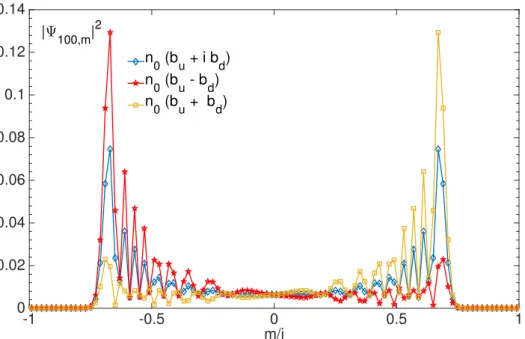
14 Chapter 1. HOMOGENEOUSQUANTUMWALKS m/j 0 0.2 0.4 0.6 0 0.05 0.1 m/j -1 -0.5 0 0.5 1 0 0.02 0.04 0.06 0.08 0.1 0.12 0.14 n 0 (bu + i bd) n 0 (bu - bd) n 0 (bu + bd) |Ψ_100,m|2

Figure 1.1:Spread of probability density of a Hadamard walk on n grid points with asymmetric initial state ™0=Pm√0,m(cL|bLi + ei ¡cR|bRi) T where (i) cL= 1,cR= 1,¡ = 0 or (ii) cL= 1,cR= °1,¡ = 0 and

symmetric initial state cL= 1,cR= 1,¡ = º/2. The spatial component is given by √0=Pm±0,m

™0, with cL= 1,cR= 1,¡ = 0, obeying to the Eqs.(1.12,1.13), the probabilities P±read:

PQW_® = (1 ± sin(2µ)cos(≥ ° ª)) (1.23) This probability distribution will be equal and lead to a left-right symmetry in position if ≥ ° ª= (2k + 1)º

2, k 2 N2. Otherwise the parameters ª and ≥ will introduce bias in the spatial probability distribution from the very first step.

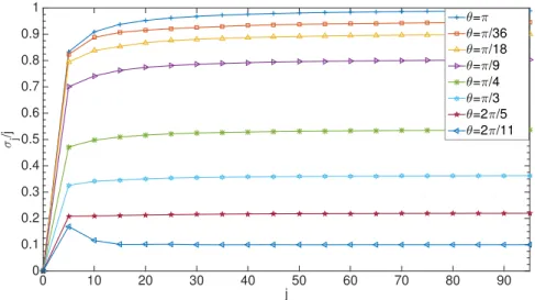
Concerning again the variance of the walk, the three Euler angles do not change qualitatively the dynamics in respect to the Hadamard case, which always remains ballistic. However, now the root of the variance æ is a function of all the three Euler angles:

æ_{/ K}µ,ª,≥j. (1.24)

A simple case can be shown taking into account, for instance, all the angles equal to zero ex-cept µ and Kµ/

p

1 ° sinµ [7]. Observe in Fig.1.4that the value of Kµdecreases as µ increases.

In particular in the limit of µ=º/2 the walker does not spread, but it is localized around the origin, therefore Kµ = 0. Conversely, if µ= kº, k 2 Z, the particle spreads with Kµ = 1.

Inter-mediate values of the variance are dominated by the interference effects, and the probability distribution spreads, after N steps, over the interval (- N cosµ, N cosµ). As in the Hadamard walk, the probability distribution decreases rapidly beyond |N cosµ|.

2_{Note that in case of Eqs.(}_1.15_,_1.16_{), the probability to find the particle in position m = ®1 starting from a}

symmetric initial state, reads P_®= (1 ® sin(2µ)cos(≥ + ª)). This probability distribution will be equal and lead to a left-right symmetry in position if ≥ + ª = (2k + 1)º

(30)

j 0 10 20 30 40 50 0 5 10 15 20 25 30

σ ∝ j

σ

j

Figure 1.2: Square root of variance of a Hadamard Walk with symmetric initial state and localized position in the origin. The slope is (1 °p1

2) 1/2_. m/j -1 -0.8 -0.6 -0.4 -0.2 0 0.2 0.4 0.6 0.8 1 0 0.02 0.04 0.06 0.08 0.1 0.12 0.14 0.16 0.18 θ = π/4 θ = π/3 θ = π/8 θ = π/16 |Ψ_100,m|2 σ ∝ (1-sinθ)1/2 j

Figure 1.3:Spread of probability density of the DTQW with symmetric initial state and different values of µ, for Æ = °º/2, ª = º/2 and ≥ = º/2.

(31)

16 Chapter 1. HOMOGENEOUSQUANTUMWALKS j 0 10 20 30 40 50 60 70 80 90 σ j /j 0 0.1 0.2 0.3 0.4 0.5 0.6 0.7 0.8 0.9 1 θ=π θ=π/36 θ=π/18 θ=π/9 θ=π/4 θ=π/3 θ=2π/5 θ=2π/11

Figure 1.4:Value of Kµfor a given µ.

1.1.5 Quantitative description

1.1.5.1 Fourier methods for the Hadamard walk

The analytical description of QWs dynamics has represented over the last few years an impor-tant field of investigation. Two methods have been extensively used: (i) the Fourier method and (ii) the combinatorial approach. In the former, the QW dynamics is studied in Fourier space in order to get a closed-form of the coin amplitude equations and, therefore, computing statistical properties of the walker. It was first introduced by Nayak and Vishwanath [32] and later by Kosik [27]. In the combinatorial approach, we shall compute the amplitude for a par-ticular position m component by summing up the amplitudes of all the paths which begin in the given initial condition and up in the same position m. This approach is also called discrete path integral approach and was developed mainly by Machida and Konno [31].

Here, we briefly recall the first method for the family of QWs obeying to Eqs. (1.12) and (1.13). Note that this could easily be extended to Eqs. (1.15) and (1.16). The closed-form of the coin amplitude is straightforward if we consider Eqs. (1.12) and (1.13) in Fourier space. Then let us look at ˆ™j,k =Pm™j,mei km Fourier transformed state of ™j,m. The finite difference

equations read: _√ ˆ √L_{j +1,k} ˆ √R_{j +1,k} ! = ei Æ √ ei (ª°k)_cosµ _ei (≥°k)_sinµ

°e°i(≥°k)sinµ e°i(ª°k)cosµ !√ ˆ √L_j,k ˆ √R_j,k ! (1.25) or more compactly ˆ™_{j +1,k}=Uk ™ˆj,k, where Uk is the Fourier transform of the unitary

opera-tor driving the walk and it is local. In order to compute the solution after N steps, we need to compute (Uk)N and this is easily accomplished if we diagonalize the unitary matrix

associ-ated with the operator Uk. A unitary matrix is always diagonalizable as a consequence of the

spectral theorem. Therefore Uk is diagonalizable:

Vk=O°1UkO (1.26)

(32)

real. Moreover, the power U_kNis simply given by Uk=O(Vk)NO°1or by: U_kN=O √ ∏1N 0 0 ∏2N ! O°1 (1.27)

To compute the solution, let us take into account as initial condition ˆ™0,k =Pm™0,mei km, where ™0,m = ±m,0|bLi. Computations of the exact expression for the Fourier-transformed

amplitudes ˆ√Land ˆ√R are straightforwards. For instance, we report the solution for the am-plitudes obeying to a Hadamard walk, that is for BH= B°º/2,º/4,º/2,º/2:

√L_j,m₌ √ 1 2º Zº °º °iei k 2p1 + cos2_k(e °i(!kj °km)_)dk ! (1.28) √R_j,m₌ µ ₁ 2º Zº °º1 + cos(k) p 1 + cos2_k(e °i(!kj °km)_)dk ∂ (1.29) where !k =sin°1(sin(k)p₂ ) and !k 2 [°º₂,º₂]. As we can see, the amplitudes for even m at odd j

vanish and the same for the odd n at even j . Having an analytical expression of ™jallows the

study of the asymptotical behavior of the probability distribution |™j,m|2. Results of this study

are extensively treated in [47], and confirm the previous qualitative description. We summa-rize here two important conclusions: (i) both amplitudes √L and √R are almost uniformly spread over the region [°j/p2, j /p2], in general over [°jKµ,ª,≥, j Kµ,ª,≥], and they decay rapidly to zero outside the region; (ii) the position probability distribution spreads as a function of j , in contrast to the standard deviation of an unrestricted CRW on a line, which is of order O(pj ).

1.2 Connections between Quantum Walks and Relativistic Wave

Equa-tions

1.2.1 Quantum walks and Feynman’s Checkerboard

In Feynman’s picture, a particle zig-zags at the speed-of-light across a spacetime lattice, flipping its chirality from left to right with an infinitesimal probability each time-step. The resulting dynamics, in the continuum limit, is the Dirac equation, with the flipping rate determined by the mass of the particle. (Strauch [43])

The Feynman’s Checkerboard was first introduced in its original version by Feynman and Hibbs [10] as a simple path integral representation for the retarded Dirac propagator in 1+1 dimensions. In this model the particle’s motion is restricted to be either forward (right) or backward (left) at the velocity of light. Feynman’s path integral results from a particular finite differencing of the massive Dirac equation in (1+1):

(@ @t ±

@ @x)√

L,R_{= i M√}R,L_. _(1.30)

where M is the real and constant mass of the fermion.

(33)

Feynman, read:

√L_j,m= √L_{j °1,m°1}+ i ˜M√R_{j °1,m+1} (1.31)

√R_j,m_{= √}R_{j °1,m+1}_{+ i ˜}M√L_{j °1,m°1} (1.32)

where ˜M = ≤M. These equations may be interpreted as following: the probability amplitude for a particle to be at (j,m) moving toward the right, is equal to the amplitude encountered at (j °1,m+1) moving toward the right plus i≤M times the amplitude encountered at (j °1,m°1) moving toward the left. Instead the probability amplitude for a particle to be at (j,m) moving toward the left, is equal to the amplitude encountered at (j ° 1,m ° 1) moving toward the left plus i ≤M times the amplitude encountered at (j ° 1,m + 1) moving toward the right. Iterating

Figure 1.5:Feynman’s Checkerboard representation in the discrete space time lattice (x, t). the finite difference Eqs. (1.32), √L,R _{may be expressed as a sum over paths leading to (j,m).}

The retarded propagator Kj,m is, therefore, the sum of number of paths, with N steps, leaving

the point m0_{in direction ¬}0_{and end at point m" in direction ¬ and switching direction B times.} Thus Kj,mcan be expressed as:

K¬¬0=X B

The convergence of Eq. (1.33) to the exact continuum propagator in the limit ≤ ! 0 is demon-strated by Jacobson and Schulman [22].

We can recognize that the probabilities (1.23) of a homogenous QW are related with what Feyn-man found for the Dirac particle of mass M. In fact, imposing µ=≤M₂ , the probability distribu-tion reads:

PQW_± º (1 ± ≤M). (1.34)

The relationship between the Feynman’s Checkerboard and QWs is even more clear if we con-sider the discrete path integral approach introduced in modeling quantum walks, for instance,

(34)

by Machida and Konno [31]. Thus, we dedicate the next section and the next chapter to un-derstand the nature of this connection.

1.2.2 Homogeneous DTQWs and Weyl equation

Differently to what Feynman did, in this section we want to investigate the formal continuous limit of DTQWs with homogeneous and static quantum coin operator BÆ,ª,≥,µ.

In order to investigate the continuous limit we first introduce a time step ¢t and a space step ¢x. We then introduce for any quantity a appearing in Eq. (1.15) and (1.16), a function ˜a defined on R+_{£ R such that the number a}_j,m _{is the value taken by ˜}_{a at the spacetime point} (tj= j ¢t, xm= m¢x). We then suppose ™(tj, xm) to be at least C2and that its characteristic

length § to be much larger than the lattice parameter ¢x. Let us consider here the equations (1.15) and (1.16): √ √L(tj+ ¢t, xm) √R(tj+ ¢t, xm) ! = BÆ,ª,≥,µ √ √L(tj, xm° ¢x) √R(tj, xm+ ¢x) ! (1.35) If the formal continuous limit exists, it will be obtained formally: (i) expanding each terms of the equations in ¢t and ¢x at fixed tjand xmand finally (ii) moving ¢t and ¢x to zero.

Let us now introduce a time-scale ø 2 R and a length-scale ∏ 2 R and an ≤ 2 R so that ø≤ ø 1 and ∏≤ ø 1. Define ¢t = ø≤ and ¢x = ∏≤±_{, where ± is a strictly positive real number,}

which traces the fact that ¢t and ¢x may tend to zero differently. The Taylor expansion of each spacetime dependent function in (1.35), up to order O(≤2), reads:

™L,R(tj+ ¢tj, xm) = ™L,R(tj, xm) + ø≤@t™L,R(tj, xm) +O(≤2) (1.36)

™L,R(tj, xm± ¢x) = ™L,R(tj, xm) ± ∏≤±@x™L,R(tj, xm) +O(≤2±)

The Eq. (1.35) then leads us to: √ √L(tj, xm) √R(tj, xm) ! + ø≤@t √ √L(tj, xm) √R(tj, xm) ! +O(≤2) = BÆ,ª,≥,µ(1 + ∏≤±@x+O(≤2±)) √ √L(tj, xm) √R(tj, xm) ! (1.37) Note that, in order to cancel the zeroth order contribution out, we have to impose that BÆ,ª,≥,µtends to the identity matrixI2of dimension 2 £ 2. Therefore the following equations must be satisfied:

ei (Æ+ª)cosµ = 1 (1.38)

ei (Æ°ª)cosµ = 1 ei (≥+Æ)sinµ = 0

The above relations imply µ = kº, Æ = (k + k+_{+ k}°_{)º, ª =(k}

+° k°)º, (k,k°,k+) 2 Z3. The angle ≥ does not enter this constraint and is therefore an arbitrary real value.

Finally, letting ≤ to zero, the Eqs. (1.37) admits formally two continuous limits: (i) one for ± > 1. In this case there is no propagation and the particle is localized at the initial condition; (ii) the most interesting case is for ± = 1 because all contributions are then of equal importance.

Let us now regard T = t/ø, X = x/∏, the equations of motion for the continuous limit of S1≤

in this simple homogeneous case read:

(35)

20 Chapter 1. HOMOGENEOUSQUANTUMWALKS ( @ @T + @ @X)√ R_{= 0} _(1.40)

Taken together, these two coupled first-order PDEs forms a system of relativistic wave equations describing massless spin-1/2 particles, otherwise known as Weyl equations. Let us remember that, in flat two-dimensional spacetime, the Clifford algebra can be represented by matrices acting on two-component spinors. This algebra admits two independent generators ∞0and ∞1, which can be represented by matrices obeying to the usual anti-commutation re-lation {∞a,∞b} = 2¥abI, where ¥ is the Minkowski metric and_Iis the Identity matrix. Consider the (non unique) representation ∞0_{= æ}

1and ∞1= °æ1æ3= iæ2, where æ1,æ2and æ3are the three Pauli matrices:

æ1= " 0 1 1 0 # , æ2= " 0 °i i 0 # , æ3= " 1 0 0 °1 # . (1.41)

The Eqs. (1.39,1.40) can be recast in the following compact form:

i ∞µ@µ™= 0 (1.42)

where @0₌ @ @T, @

1₌ @ @X.

1.2.3 Publication: "Massless Dirac Equation from Fibonacci Discrete-Time Quan-tum Walk"

This publication is a joint effort between the collaboration of the JSPS fellow Di Molfetta with the Shikano group, and the internship of two undergraduate Australian students, Lauchlan Honter and Ben Luo, from The University of Western Australia. We present two modified ver-sions of the aperiodic quantum walk introduced by Ribeiro et al. [40], as a simple but non trivial case of the continuous limit with a homogeneous and periodic unitary step operator.

We introduce two models of DTQWs. The first, labeled FDTQW-I, is a generalized Hadamard coin B(µj) = Bjfollowing the infinite Fibonacci sequence, as below:

B_{j +1}_{= B}jBj °1 (1.43)

where B0 = B(Æ) and B1 = B(Ø)B(Æ). We found that this sequence when applied to the coin operator is six-steps periodic. The formal continuous limit of the stroboscope of period six co-incides with a ballistic equation that recover the Weyl equation in two spacetime dimension.

In the second case, FDTQW-II, the Fibonacci sequence is followed by the QW’s step opera-tor_U=_TB:

Uj +1=UjUj °1 (1.44)

where_U0=TB(Æ) andU1=TB(Ø)TB(Æ). In this case the sequence is no longer periodic but aperiodic as Ribeiro et al. [40] proved in his paper. In particular they showed that this model displays a sub ballistic behavior. What we prove is that if we truncate the Fibonacci sequence in FDTQW-II the behavior is no longer sub-balistic and display a standard propagative behavior. There still remains a problem concerning the type of transition occurring when the periodicity FDTQW-II increases towards infinity, and the mechanism by which the dynamical behavior of the periodic extension changes into that of the infinite sequence [40].

(36)

DOI 10.1007/s40509-015-0038-6

R E G U L A R PA P E R

Massless Dirac equation from Fibonacci discrete-time

quantum walk

Giuseppe Di Molfetta · Lauchlan Honter · Ben B. Luo · Tatsuaki Wada · Yutaka Shikano

Abstract Discrete-time quantum walks can be regarded as quantum dynamical simulators since they can sim-ulate spatially discretized Schrödinger, massive Dirac, and Klein–Gordon equations. Here, two different types of Fibonacci discrete-time quantum walks are studied analytically. The ﬁrst is the Fibonacci coin sequence with a generalized Hadamard coin and demonstrates six-step periodic dynamics. The other model is assumed to have three- or six-step periodic dynamics with the Fibonacci sequence. We analytically show that these models have ballistic transportation properties and continuous limits identical to those of the massless Dirac equation with coin basis change.

Keywords Quantum Walk· Massless Dirac equation · Quantum Simulation

G. Di Molfetta, L. Honter, and B. B. Luo are equally contributed to this work. G. Di Molfetta· L. Honter · B. B. Luo · Y. Shikano

Research Center of Integrative Molecular Systems (CIMoS), Institute for Molecular Science, Natural Institutes of Natural Sciences, 38 Nishigo-Naka, Myodaiji, Okazaki, Aichi 444-8585, Japan

G. Di Molfetta

LERMA, Observatoire de Paris, PSL Research University, CNRS, Sorbonne Universités, UPMC Univ. Paris 6, UMR 8112, F-75014 Paris, France

e-mail: giuseppe.dimolfetta@ens.fr L. Honter· B. B. Luo

School of Physics, The University of Western Australia, 35 Stirling Hwy, Crawley, Perth, WA 6009, Australia T. Wada

Department of Electrical and Electronic Engineering, Ibaraki University, 12-4-1 Nakanarusawa, Hitachi, Ibaraki 316-8511, Japan Y. Shikano ( )

Institute for Quantum Studies, Chapman University, 1 University Dr., Orange, CA 92866, USA e-mail: yshikano@ims.ac.jp

(37)

G. Di Molfetta et al.

1 Introduction

Discrete-time quantum walks (DTQWs) are defined as quantum-mechanical analogues of classical random walks. The concept of DTQWs was first considered by Feynman [1] and then introduced in greater generality by Refs. [2–4]. They have been realized experimentally in Refs. [5–20] and are important in many fields, from fundamental quantum physics [15,21–23] to quantum algorithm [24–26] and condensed matter physics [27–37]. Previously, it has been shown that several DTQWs on a line admit a continuous limit identical to the propagation equations of a massive Dirac fermion [39–43] and those of massless Dirac fermion equations [21,39]. Furthermore, the relationship between DTQWs and artificial electric and gravitational fields has been shown [21,44]. Thus, DTQWs can be regarded as quantum dynamical simulators [39,40]. Additionally, it is well known that the classical random walk leads to a diffusive behavior characterized by the time evolution of the standard deviation, with σ (t)_{∼ t}1/2_,

while the standard DTQW leads to ballistic behavior, as σ (t)_{∼ t. Further, the standard DTQW can be considerably} enriched by generalizing the quantum coin operator and arranging it along different sequences. It has already been shown that quasi-periodic coin sequences induced by the Fibonacci sequence lead to sub-ballistic behavior, whereas random sequences lead to diffusive spreading [48–50]. Here, we consider two different Fibonacci DTQWs with periodic coin sequences. The first model (FDTQW-I) considers a time-dependent quantum coin following the Fibonacci sequence, while the second model (FDTQW-II) considers a modified version of the unitary operator first defined in Ref. [48], where the Fibonacci sequence is applied to the step operator. We show numerically and analytically that the continuous limit of these models reduces to a massless Dirac equation in (1_{+ 1) dimensions.}

2 Discrete-time quantum walk with Fibonacci sequence coin

Let us consider the two-dimensional spin state "m, j ∈ C2, spanned by the orthonormal basis (bu,bd), and defined

by its discrete one-dimensional position m_{∈ Z and discrete time j ∈ N}0. The standard DTQW’s time evolution is

given by the application of the quantum coin operator (QCO) ˆCon "m, j = um, jbu+ dm, jbd =

✓_u

m, j

dm, j

◆

, followed by the chiral-dependent translation operator ˆT, which is defined as:

✓ um−1, j dm+1, j ◆ = ˆT ✓ um, j dm, j ◆ . (1)

Here, we introduce the simplest quantum coin, the generalized Hadamard coin, which is expressed as:

ˆC(θ) =✓cos(θ)_sin(θ) _{− cos(θ)}sin(θ) ◆, (2)

where θ _{∈ [0, 2π]. The one-step discrete time evolution is then given by:} ✓ um, j+1 dm, j+1 ◆ = ˆT ˆC(θ) ✓ um, j dm, j ◆ . (3)

First, we consider FDTQW-I, which is the simplest case as only the QCO is defined as a Fibonacci series. Here,

ˆUj = ˆT ˆCj , j ∈ N0 , ˆCj+1= ˆCj ˆCj−1, (4)

with the initial conditions

ˆC0 = ˆC(α) , ˆC1= ˆC(α) ˆC(β), (5)

where j is the time step. On considering the DTQW acted upon by the Fibonacci coin series, we analytically find that the time evolution of the coin is cyclic with period 6. These coin operators then reduce to,

(38)

ˆC0 = ✓ cos(α) sin(α) sin(α) _{− cos(α)} ◆ , ˆC1 = ✓_cos(α − β) − sin(α − β) sin(α_{− β)} cos(α_{− β)} ◆ , ˆC2 = ✓_cos(2α − β) sin(2α_{− β)} sin(2α_{− β) − cos(2α − β)} ◆ , ˆC3 = ✓ cos(α) sin(α) sin(α) _{− cos(α)} ◆ , ˆC4 = ✓ _cos(α − β) sin(α_{− β)} − sin(α − β) cos(α − β) ◆ , ˆC5 = ✓_cos(β) _sin(β) sin(β) _{− cos(β)} ◆ . (6)

Here, the collection Wn

j = ("m,k)m∈Z,k=nj is defined for j ∈ N and n ∈ {0, 1, 2, 3, 4, 5}, and represents the state

of the walk at time k _{= nj. For any given n we define S}n _{= (W}n

j)j∈Z, where Sn represents the entire history of the walk observed through a stroboscope of period n. Successive application of the 6 unitary operators to an initial state then gives the stroboscopic recursion equations for S6_{. The discrete-step equations for S}6_read

um, j+6= 3 X k=−3 A2k(α, β)um+2k, j+ B2k(α, β)dm+2k, j , (7) dm, j+6= 3 X k=−3 B_−2k(−α, −β)um+2k, j + A−2k(−α, −β)dm+2k, j . (8)

Here, the index k_{∈ {−6, −4, −2, 0, 2, 4, 6} and the coefficients A}k, Bk ∈ R are explicitly given as

A₋₆_{= c}_α2cβc2α−βc2α−β (9) A₋₄_{= −}1 4cαc 2 α_−β(cα_−2β+ 3c3α−2β− 5cα+ c3α) A₋₂₌ 1 16(−6c2(α−β)+ 4c4(α−β)− c2(α+β)− c2(α−2β) + 2c4α−2β− c6α−2β+ c6α−4β− 2c4α− 2c2β+ 6) A0 = 1 4c 2 α−β(−6c2(α−β)+ c4α−2β− 2c2α + c4α+ c2β+ 5) A2 = 1 8c 2 α−β(6c2(α−β)− 3c4α−2β− 2c2α+ c4α+ c2β − 3) A4 = 1 2s2αsβc 2 α−βc2α−β A6 = 0 B₋₆₌ 1 2s2αcβcα2−βc2α−β (10) B₋₄₌ 1 8 s2αsβ(sβ− s4α−3β)+ cβ(3s2α−β− s4α−β+ 3s4α−3β− s6α−3β) B₋₂₌ 1 8 ⇣ (c2α− 3)s4α−4β− 2s4αc2α−β ⌘

(39)

G. Di Molfetta et al. B0 = _{16 −}1 s2α−4β+ 4s4α−4β+ s6α−4β+ 2cα(sα_+2β− sα−2β− 3s3α−2β+ s5α−2β)− 2s2α + 2s4α B2 = −₁₆1 cα(s3α−4β+ 3s5α−4β + 8sα3c2α−2β+ 4sα− 2s3α) B4= −c2αsβc2α_−βc2α−β B6= 0

with cθ := cos(θ) and sθ := sin(θ).

Let us define the time and space variables, tj = j't and xm = m'x, where 't and 'x are the time and space

steps, respectively. As 't and 'x tend to zero, this allows us to take a Taylor expansion of the recursion relations for the DTQW and, hence, derive a pair of partial differential equations (PDEs). To take the continuous limit, we define

't = ϵ ,

'x = ϵγ , (11)

where ϵ is an infinitesimal and γ > 0 is a scaling parameter. The difference between the two expressions is to account for the fact that 't and 'x may tend to 0 differently. Then, taking a Taylor expansion about ϵ up to the leading orders of Eqs. (7) and (8), we obtain the following

u(x, t)_{+ 6ϵ∂}tu(x, t)= u(x, t) + ϵγ ( p1∂xu(x, t)+ p2∂xd(x, t))+ O(ϵ2), (12)

d(x, t)_{+ 6ϵ∂}td(x, t)= d(x, t) + ϵγ ( p2∂xu(x, t)− p1∂xd(x, t))+ O(ϵ2), (13) where p1= 3 X k=−3 2k 6 A2k(α, β)= − 1 6(c4α−2β+ 2c2α+ c2β + 2), (14) p2= 3 X k=−3 2k 6 B2k(α, β)= − 2 3(s2αc 2 α−β). (15)

Choosing scaling of γ _{= 1 and then taking the limit as ϵ → 0, we obtain the following pair of PDEs:} ∂tu(x, t)= p1∂xd(x, t)+ p2∂xu(x, t),

∂td(x, t)= p2∂xd(x, t)− p1∂xu(x, t).

(16) This set of equations can be then be recast, such that

I∂t"+ P∂x" = 0 , P = ✓ p1 p2 p2 −p1 ◆ , (17)

whereI is the 2 × 2 identity matrix. To diagonalize the operator acting on ", we perform a change of basis from (bu,bd) to the new basis, (bu,bd), with " = ubu + dbd. The new basis components are

bu = 1_Z ✓ _p 2 ω− p1bu+ bd ◆ , (18) bd = 1 Z ✓ − p2 ω+ p1bu+ bd ◆ , (19)