The dynamics and kinematics of the coastal boundary layer off Long Island

by

NEAL ROBERT PETTIGREW A.B., Dartmouth College (1972) M.S., Louisiana State University (1975)

SUBMITTED IN PARTIAL FULFILLMENT OF THE REQUIREMENTS FOR THE DEGREE OF

DOCTOR OF PHILOSOPHY

at the

MASSACHUSETTS INSTITUTE OF TECHNOLOGY and the

WOODS HOLE OCEANOGRAPHIC INSTITUTION December, 1980

('&e

_F1'.ot

Yi

f'

'

'i"

Joint Program in Oceanography, Masachusetts Institute of Technology - Woods Hole Oceanographic Institution, and Department of Earth and Planetary Sciences, and Department of Meteorology, Massachusetts Institute of Technology, December, 1980.

Certified by...

Certified by ...__D ...

- Thesis Supervisor

Accepted by... Chairman, Joint Oceanography Committee in Earth Sciences,

Massachusetts Intsitute of Technology - Woods Hole Oceanographic

Institution. ARCHIVES MASSACHUSETTS INSTITUTE

OF TECHNOLOGY

FEB 1 0 1981

by

NEAL ROBERT PETTIGREW

Submitted to the Massachusetts Institute of Technology - Woods Hole Oceanographic Institution Joint Program in Oceanography on December 30, 1980, in partial fulfillment of the requirements for the degree of Doctor of Philosophy

ABSTRACT

Data from the COBOLT experiment, which investigated the first 12 km off Long Island's south shore, are analyzed and discussed. Moored cur-rent meter records indicate that the nearshore flow field is strongly polarized in the alongshore direction and its fluctuations are well cor-related with local meteorological forcing. Complex empirical orthogonal function analysis suggests that subtidal velocity fluctuations are baro-tropic in nature and are strongly influenced by bottom friction.

Wind-related inertial currents were observed within the coastal boun-dary layer (CBL) under favorable meteorolgical and hydrographical condi-tions. The magnitude of these oscillations increases with distance from shore, and they display a very clear 1800 phase difference between sur-face and bottom layers. Nearshore inertial oscillations of both velocity and salinity records appear to lead those further seaward, suggesting local generation and subsequent radiation away from the coast.

The response of the coastal zone to impulsive wind forcing is dis-cussed using simple slab and two-layer models, and the behavior of the nearshore current field examined. The major features of the observed inertial motions are in good qualitative agreement with model predic-tions. It is found that, in a homogeneous domain, the coastal boundary condition effectively prohibits inertial currents over the entire coastal zone. In the presence of stratification the offshore extent of this pro-hibition is greatly reduced and significant inertial currents may occur within one or two internal deformation radii of the coast. The "coastal effect", in the form of surface and interfacial waves which propagate

away from the coast, modifies the "pure" inertial response as it would exist far from shore. The kinematics of this process is such that a 180 phase difference between currents in the two layers is characteristic of the entire coastal zone even before the internal wave has had time to traverse the CBL. It is also suggested that, for positions seaward of

several internal deformation radii, interference between the surface and internal components of the coastal response will cause maximum inertial

amplitudes to occur for t > x/c₂, where c2 is the phase speed of the

internal disturbance.

The hydrographic structure of the CBL is observed to undergo fre-quent homogenization. These events are related to both advective and mixing processes. Horizontal and vertical exchange coefficients are estimated from the data, and subsequently used in a diffusive model which accurately reproduces the observed mean density distribution in the nearshore zone.

Dynamic balance calculations are performed which indicate that the subtidal cross-shore momentum balance is very nearly geostrophic. The calculations also suggest that the longshore balance may be reasonably represented by a steady, linear equation of motion which includes sur-face and bottom stresses.

Evidence is presented which shows that variations in the longshore wind-stress component are primarily responsible for the energetic fluc-tuations in the sea surface slope along Long. Island. Depth-averaged velocities characteristically show net offshore transport in the study area, and often display dramatic longshore current reversals with dis-tance from shore. These observations are interpreted in terms of a steady circulation model which includes realistic nearshore topography. Model results suggest that longshore current reversals within the CBL may be limited to the eastern end of Long Island, and that this unusual flow pattern is a consequence of flow convergence related to the pres-ence of Long Island Sound.

Thesis Supervisor: Dr. Gabriel T. Csanady Title: Senior Scientist

who are both my strength and my weakness

I would like to express my gratitude to my thesis advisor Dr. Gabriel T. Csanady for his patience, support, and guidance. His editorial acumen

substantially improved this manuscript, and his personal kindness and optimism were a calming influence during my years as a graduate student.

In addition to the members of my thesis committee, Drs. N.G. Hogg, P.W. May, and J.F. Price provided useful discussions and critical reading of early drafts of this thesis.

Dr. T.S. Hopkins, Jim Lofstrand, and Catherine T. Henderson, all of the Brookhaven National Laboratory, kindly provided most of the data used in this work as well as helpful evaluations of its accuracy. Bert Pade, my companion of many days aboard the R.V. COBOLT, was primarily

respon-sible for the collection of the transect profiles. James H. Churchill provided assistance in several of my programming efforts.

I would like to thank Dr. Paul W. May, office-mate and friend, for inumerable scientific and philosophical discussions. His personal and professional advice invariably proved valuable.

Doris Haight cheerfully and expeditiously typed the first draft of this manuscript, and May Reese provided careful proofreading and typed the numerous equations in chapter III. Karin Bohr patiently explained the mysteries of the word processor, and graciously interrupted her schedule in order to type the equations in chapters IV and VI.

I thank Joyce Csanady, Eloise Soderland, and May Reese for their maternal instincts, and "Data Dollies" Terry McKee, Carol Mills, and Nancy Pennington for cheerfully providing programming assistance and strong shoulders to cry on.

I have benefitted from many friendships with the students and staff of the Woods Hole Oceanographic Institution and thank them all for thei.r good humor and camaraderie. In particular, I am grateful to Jerry

Needell and Ping-Tung Shaw who frequently served as touchstones for many of my ideas.

Finally I owe a special debt of gratitude to my wife Trish for draft-ing most of the figures in this thesis, and for her many sacrifices as a student's spouse. Special thanks also to my baby daughter Sarah Morrow for a much needed vote of confidence when, at age 14 months, she came upon a pad of my scribblings and proclaimed it "book".

This work was supported by the Department of Energy through contract no. DE-AC02-EV10005 entitled Coastal-Shelf Transport and Diffusion.

ABSTRACT . ... 2

ACKNOWLEDGEMENTS . ... 5

TABLE OF CONTENTS ... 7... 7

CHAPTER I THE COASTAL BOUNDARY LAYER TRANSECT EXPERIMENT 1.1 Introduction ... 10

1.2 The concept of the coastal boundary layer .... 1313... 1.3 COBOLT deployments and experimental configurations ... 15

1.4 Instrumentation ... 20

1.5 Calibration and quality control ... 26

1.6 Data reduction ... 29

CHAPTER II THE SPECTRAL DESCRIPTION OF THE VELOCITY FIELD 2.1 Introduction ... 31

2.2 Cross-shore variation of energy ... 35

2.3 The rotary-spectral description ... 42

2.4 The vertical structure of the flucuating currents ... 49

CHAPTER III INERTIAL CURRENTS IN THE COASTAL ZONE: OBSERVATION AND THEORY 3.1 Introduction ... 57

3.2 Wind stress and inertial currents ... 59

3.4 3.4.1 3.4.la 3.4.lb 3.4.1c 3.4.1d 3.4.2 3.4.3 3.5 CHAPTER IV 4.1 4.2 4.3 4.4 4.5 4.5.1 4.5.2 4.6 CHAPTER V 5.1 5.2 5.2.1 5.3

A two-layer model of coastal response to impulsive wind.. Offshore wind forcing: the delta function... Interfacial response... Current response... The importance of stratification ...

Interference phenomena and offshore amplification... Offshore wind forcing of finite duration... Forcing by longshore winds... Summary . ...

HYDROGRAPHIC VARIABILITY IN CBL

Introduction...

Mixing of the nearshore water column... Shoreward advection of homogeneous water... Advection and mixing... Advective-diffusive exchange coefficients ...

Calculation of horizontal exchange coefficients... Estimation of the vertical exchange coefficient... A diffusive equilibrium density distribution...

OBSERVATION OF NEARSHORE CURRENTS AND SEA LEVEL Introduction... Variations in the alongshore sea level gradient.. Variations on monthly and seasonal time scales... Current meter observations in the CBL...

SLOPE ... ... ... ... 71 78 80 84 89 91 96 111 112 114 116 126 129 133 137 139 141 149 1 52 167 170

5.3.1 Depth-averaged longshore currents ... 174

5.3.2 Depth-averaged cross-shore flow ... 181

5.4 Evidence of mean flow against the pressure gradient ... 187

5.5 Momentum balance calculations ... 190

5.5.1 Error analysis ... 192

5.5.2 The linear time dependent dynamic balance ... 194

5.5.3 The steady dynamic balance ... 202

5.6 A comparison of linear and quadratic bottom friction... 204

5.7 Summary ... 209

CHAPTER VI MODELS OF STEADY AND QUASI-STEADY FLOW IN THE CBL 6.1 Introduction ... 210

6.2 Nearshore parallel flow ... 211

6.3 The arrested topographic wave ... 214

6.3.1 The influence of nearshore topography ... 217

6.4 Wind-stress variation in shoreline coordinates ... 225

6.5 The matched exponential bottom profile ... 228

6.5.1 The character of matched exponential model solutions ... 234

6.5.2 Comparison with observation ... 242

6.6 Summary ... 248

APPENDIX: Two-layer coastal response to longshore forcing ... 250

REFERENCES ... 255

THE COASTAL BOUNDARY LAYER TRANSECT EXPERIMENT

1.1 Introduction

The shallow coastal regions of the worlds oceans differ from deeper water environments dynamically, geologically, biologically, and in the

physical-chemical properties of their associated water masses. In fact, within these shallow regions themselves, subregions may be identified

(figure 1.1) such as the continental shelf break, outer shelf, inner shelf, coastal boundary layer, and surf zone, which are in many respects distinct (see Beardsley, Boicourt, and Hansen, 1976) and in some cases almost independent from one another. Yet despite these interesting and important differences, and to some extent because of them, the physical oceanography of these shallow marginal waters has historically remained

largely overlooked. Only within the last decade has this trend been reversed with the commencement of a dramatic increase of interest in and understanding of the dynamics and kinematics of the world's coastal seas.

Advances in current meter and mooring technology, together with the recent surge of interest in the physical oceanography of the U.S. con-tinental shelf regions, have resulted in the institution of extensive field programs involving moored instrument arrays often in conjunction

o

c

E

o

=

v,

0

0

0

0

0

_

r-(w)

qda(]

with densely spaced hydrographic surveys. Examples of these concerted efforts are the MESA project (Mayer et al., 1979), Coastal Upwelling Experiments 1 and 2 (Kundu and Allen, 1975), the Little Egg Inlet

Exper-iment (EG&G, 1975), and the New England Shelf Dynamics ExperExper-iment (Flagg et al., 1976). The excellent returns associated with these initial efforts have allowed characterization of both the mean and fluctuating

portions of the scalar and vector fields found in inner shelf and deeper coastal environments. In addition, this rapid increase in basic obser-vational information has sparked new theoretical interest with its

at-tendant advancement in the understanding of the underlying dynamics of the shelf region. For excellent reviews of these observational and theoretical developements see Allen (1980), Csanady (1981), Mysak (1980) and Winant (1980).

In the very shallowest waters of the coastal region, within approx-imately 100 meters of the runup limit, is the wave-driven surf zone.. This region has historically been the subject of both varied and

vigor-ous study, primarily by civil and coastal engineers, and as such pos-esses its own elaborate literature. The dynamics and the unique qual-itative flow structure within this zone are fairly well known although their relationship to deeper water processes is still an intriguing and unsettled question.

Between the surf zone and the inner shelf is a region often called

the coastal boundary layer which has been least studied, is least under-stood, and which may prove to be of greatest practical importance to an environmentally concerned technological society. This band of water,

extending from the seaward limit of the surf zone to order ten kilo-meters from the coast, is the subject of this thesis. The author hopes to illuminate its dynamics and to achieve its local characterization for a fairly typical eastern seaboard environment off Long Island's south shore.

1.2 The concept of the coastal boundary layer

The conceptual evolution of the coastal boundary layer (CBL) may be traced to investigations of the North American Great Lakes dating back some fifteen years. One of the first clear distinctions between flow conditions close to the beach and those further offshore was drawn by Verber (1966). As a result of a large scale experiment in Lake Michigan

it was noted that "straightline" along-isobath flow always occurred nearshore while mid-lake currents were characterized by horizontally

isotropic near-inertial oscillations. In addition, many investigators reported that the large thermocline displacements associated with the

upwelling events long observed in the Great Lakes were confined to a nearshore band some 10 kilometers in width. After the advent of the International Field Year on the Great Lakes in 1972, detailed coastal zone observations (Csanady, 1972a,b) left little doubt that the near-shore band was posessed of a current climatology quite different from that in deeper water, and that the thermal field and its fluctuations were also very different from those present at reatpr distance from the

coastal boundary. These observational facts formed the foundation of the CBL both as a conceptual and a theoretical construct. A more

detailed review of the developement Coastal Boundary Layer concept is given by Csanady (1977b).

The Great Lakes experiments ave yielded observational and theoret-ical results of sufficient generality to invite application to different and more complex environments. The most enticing course of action, and perhaps the greatest leap of faith as well, is the wholesale transfer-ence of the Coastal Boundary Layer concept with all its lore directly to

nearshore oceanic environments. Any such application is bound to be complicated by the additional influences of vigorous tidal fluctuations

(May, 1979) as well as interaction with larger scale flow features of the continental shelf and perhaps even the general circulation of the deep ocean. In any event the physical factors which served to differen-tiate the CBL from interior regions in the Great Lakes will also be operative and apply powerful dynamical constraints on motions in the oceanic boundary layer as well. In something like descending order of

importance, these factors are:

1) The coastal boundary constraint which prohibits net cross-shore transport at the coast;

2) The seaward deepening of the water column which results in the generation of powerful vorticity tendencies in association with cross-isobath flow;

3) The general shallowness of the water column which amplifies the importance of frictional effects;

4) The seasonal occurrence of strong stratification which concentrates longshore momentum in the surface waters and leads to dramatic offshore variations in scalar and vector fields over horizontal scales of the baroclinic deformation radius.

It was the purpose of the Coastal Boundary Layer Transect (COBOLT) experiment to discover to what extent and in what manner these con-straints continue to operate in the face of additional and complicating

influences in the oceanic environment.

1.3 COBOLT deployments and experimental configurations

Although continental shelf experiments have sometimes included occa-sional moorings within the CBL (eg. CUE 1, CUE2) the COBOLT experiment is the first study specifically designed with sufficient resolution to investigate the temporal and spatial complexities of the oceanic near-shore band. The project, which represents a six year (1974-1979) joint effort between the Woods Hole Oceanographic Institution and the Brook-haven National Laboratory (BNL), was fielded at Tiana Beach on Long

Island's south shore. The field site shown in figure 1.2 was chosen largely because it represents a fairly typical long straight section of

o o 1 e n rJ C) -, -o r, E . r0 a, .--_aP ,r-_CL LU OJ LL II r

coastline without significant topographic irregularities, as well as enjoying convenient access through the nearby (approximately 6 km

distant) Shinnecock Inlet. While it was hoped that the simple offshore bottom topography normally associated with barrier beaches would sim-plify modeling efforts, several potentially complicating local features should be noted. First and foremost is the presence of Long Island Sound which is known to have a major influence upon the tidal currents (Swanson, 1976; May, 1979), the local hydrography (Ketchum and Cnrwin, 1964), and may perhaps affect wind-driven currents as well. The close proximity of the Shinnecock Inlet may also have some effect upon the

study area, although through the analysis of airborne radiation thermo-metric data, Powell and SethuRaman (1979) have concluded that any

influ-ence of the inlet upon scalar variables within the COBOLT region is quite minor.

The COBOLT experiment generally consisted of two main oceanographic components; a moored array collecting time series measurements of tem-perature, conductivity, and velocity, and a program of daily (weather permitting) "shipboard" surveys. Experimental periods were typically of one month's duration, and under full operation four moorings were de-ployed at 3, 6, 9 and 12 km from shore employing a combined total of 16 principal instrument packages. Each sensor package recorded conduc-tivity, temperature, and orthogonal velocity components. For the three outer moorings, instrument packages were located at nominal depths of 4, 8, and 16 meters below mean sea level, plus one mounted 2.4 meters above the local bottom. The shallowest mooring (at 3 km) carried its sensors

at 4, 8, 12 meters below the surface, and 2.4 meters above the bottom. In addition, throughout the experiments as many as four additional supplementary temperature sensors per mooring were mounted at positions between the primary sensor locations. For clarity and compactness of notation, when referring to multiple mooring experiments offshore pos-itions will be numbered 1-4 progressing seaward. Vertical pospos-itions will also be denoted 1-4 numbered from the shallowest to the deepest instrument position. The convention will be mooring number followed by vertical position number so that, for instance, the number pair (3,2) refers to measurements at level 2 (8 m depth) on mooring 3 approximately 9 km from shore.

In order to provide increased spatial resolution, daily surveys were conducted at permanently maintained anchor stations along a transect coincident with the mooring array. These stations were located at 1 km

intervals out to 8 km, and at 2 km intervals thereafter, to a total distance of 12 km from the shoreline. Figure 1.3 illustrates a typical experimental configuration as well as the local bottom topography.

Meteorological information was collected at the 22 meter Tiana Beach tower and/or on site at BNL atop a 110 meter tower some 35 km distant from the field experiment.

In its initial operation in 1974, the COBOLT program was limited to

daily surveys. In September 1975 however, in addition to the surveys, one pilot mooring which collected time series measurements was success-fully deployed. Preliminary analysis of the current meter data from this experiment was reported by Scott and Csanady (1976). The summer of

0 co (D I N 0

(w)

d

CO

d

z

0~~~

E

2

O

*

~

~

1976 was scheduled to be the first full deployment of the COBOLT moorina array but heavy damage due to hurricane Belle together with technical problems precluded the collection of useful data. In an independent experiment in October-November of that same year however, BNL was able to successfully maintain a single mooring in the same region during a very interesting period of flow. These data, as reported by Scott et. al. (1978), represent an important addition to the COBOLT data set and are therefore included in the discussions which follow.

Full deployments occurred during May 1977, March 1978, and August 1978 representing a successful monitoring of the CBL during respective periods of spring warming, unstratified conditions, and mature strati-fication. Table 1.1 summarizes the data returns from the mooring pro-gram during all experiments, while figure 1.4 indicates the dates of shipboard surveys, the occurrence of significant data gaps, and start and stop (failure) times for individual buoys.

1.4 Instrumentation

The moorings employed in COBOLT are of the Shelton spar buoy type which were specifically designed for use in coastal environments (see Lowe, Inman, and Brush, 1972). It is constructed of sections of .5 cm diameter PVC pipe joined together by universal joints which allow free articulation while maintaining torsional rigidity. The spar buoy, which has large positive buoyancy, is anchored by the massive (900 kg) battery

TABLE 1.1

Data Returns from COBOLT Mooring Program

Mooring no. Position

Depth of useful current meters Sept.,1975 Oct.,1976 May, 1977 Mar., 1978 Aug., 1978 4 11 km 4 11 km 2 3 4 1 3 6 km 9 km 12 km 3 km 9 km 1 2 3 4 3 km 6 km 9 km 12 km 4, 16, 30 m 4, 8, 16, 30 m 4, 8, 16, 25 8, 16, 28 m 4, 8, 16, 30 4, 8, 4, 8, 12, 18 16, 28 4, 8, 12, 18 4, 8, 16, 25 8, 16, 28 m 4, 8, 16, 30 m m m m m m m Date

/)

i-

0

5-0

I

I n

-O

F

@

4-m

J)

c-0

0)

:D

0)

r.X

A:

pack necessary to power sensors, the in-situ data processor, and the telemetry system.

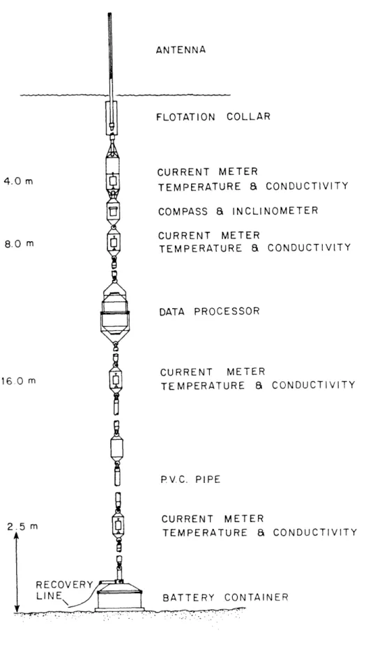
Figure 1.5 shows a typical mooring configuration containing four main instrument packages (which measure temperature, conductivity, and velocity), one pressure sensor, a compass, a pair of orthogonally moun-ted inclinometers, a data processing unit, and the telemetry receiver-transmitter. In operation, output from all sensors is low pass filtered

in real time with a 5 second time constant and the results continuously integrated by the data processor. Upon scheduled interrogation, the buoy transmits the integrated (averaged) data to a computer on site at

BNL and restarts the integration. For a more detailed technical decrip-tion of the mooring and telemetry system see Dimmler et. al. (1976).

The sensor packages used in all COBOLT deployments consisted of an inductance conductivity cell, a thermistor, and either a Marsh-McBirney 711 or 555 electromagnetic current meter. Both models of current meter feature an orthogonal set of single axis electrodes, the difference being in the geometry of the probes on which the electrodes are mounted. The 555 employs a 2.5 cm spherical probe while the 711 uses a 2.2 cm diameter cylindrical configuration. In both cases the electrodes pro-trude 3 mm from the probe surface. The principles of operation and some

operational properties of these current meters are discussed by Cushing (1976). Figure 1.6 shows the configuration of the instrument package mounted within its stainless steel cage.

ANTENNA FLOTATION COLLAR CURRENT METER TEMPERATURE 8 CONDUCTIVITY COMPASS a INCLINOMETER CURRENT METER

TEMPERATURE & CONDUCTIVITY

DATA PROCESSOR CURRENT METER TEMPERATURE 8 CONDUCTIVITY PV.C. PIPE CURRENT METER

~~~~t

Figure 1.5 COBOLT mooring confiqguration.

4.C 8. 16 0 m 2.5 m t, t UNUUL I IV I I

Moored instrument package

CIt'Q- LGG)

Cj& 1.

0,p0

1.5 Calibration and quality control

In spite of the design sophistication of the COBOLT data acquisition

system, and to some extent because of it, there have been and continue to be failures of individual instruments and even whole moorings. In addition, some concerns have arisen about the quality of the initial data returns.

Perhaps the most chronic problem has been with significant zero off-sets associated with conductivity sensors. Despite repeated and consis-tent calibrations these instruments have not always measured salinity consistently from one position to another. Under field conditions, sen-sors which were otherwise performing satisfactorily, have in rare in-stances exhibited offsets as high as 2 0/o (translated into terms

of salinity). Two independent procedures have been applied to correct errant salinity values. The simpler procedure was to introduce constant offsets sufficient to eliminate any calculated density inversions. This procedure is rendered quite effective by the fact that the water column is characteristically observed to homogenize quasi-periodically within the study area. The second procedure involved statistical comparison of salinity data with the STD surveys taken daily along the mooring tran-sect. This method virtually assures a consistent reference between

instrument positions and was used whenever statistically reliable cor-rections could be made. The fact that the results of both methods were

in close agreement somewhat allays the fear customarily associated with such "tampering". In general salinty measurements are considered to he

good to within + 0.2 ppt based upon repeated calibration runs (Hopkins et al., 1979). In any case it will usually he the time behavior rather than the absolute value of salinity which is of greatest interest in this study.

Some concern about the quality of the velocity data arose as a re-sult of the 1976 Current Meter Inter-Comparison Experiment (CMICE) as reported by Beardsley et. al. (1977). This experiment was oriqinallyv

conceived as a test of the performance of existing mooring-current meter systems against one another. Two COBOLT Shelton spars were compared in this instance to more conventional taut rope moorings employing a var-iety of mechanical current meters which sampled speed and direction independently.

The experiment was conducted in the COBOLT study area approximately 6 km offshore of Tiana Beach, Long Island. An array of six moorings were deployed in a line parallel to the coast, spanning one kilometer alongshore. Although no single mooring-current meter combination con-sistently outperformed the others, several sources of error were iden-tified for the COBOLT instrumentation. They are:

1) Compass error;

2) Misalignment of sensor packages due to slight differences in construction at the moorings articulating joints;

4) Speed and direction errors due to inaccurate gain adjustment;

5) Speed and direction errors due to the non-cosine response of the velocity sensors.

After the CMICE experiment, a concerted effort was made by BNL to upgrade the performance of their system. Problem 2 was easily corrected

prior to the May 1977 launch, and model 215 Digi Course Optically Scan-ned Magnetic Heading Sensors (resolution + 1.4 degrees) were installed before the March 1978 experiment replacing earlier versions which had

proved unreliable. Extensive calibrations at the NOAA tow tank facility in Bay St. Louis, Mississippi, including determinaton of the individual non-cosine response for each current meter, were undertaken in order to

address problems 3-5.

No attempt has been made to correct for the vertical non-cosine

res-ponse associated with the tilting of the mooring under the influence of strong flow conditions. Tilt records from the Humphreys Inc. inclino-meters (resolution 0.2 degrees) show extreme values of less than 20

degrees for all moorings, and inclinations even as great as 10 degrees are only occaissionally observed. The deviations from a simple cosine correction based upon the hourly averaged orthogonal tilt records, are clearly negligible for the magnitude of the observed angles.

Despite the corrections applied, an uncertainty in measured velocity remains of 1 cm/sec for each axis, and 5 degrees in orientation (Hopkins

et al., 1979). Based upon four calibration runs on each of 24 thermis-tors, Hopkins et. al. estimate the uncertainty in temperature as 0.02 degrees Celsius. While no checks were made on the pressure sensors, manufactuers specifcations indicate that they are accurate to better than 1.5 cm of water.

1.6 Data reduction

The first step in the data processing routine was the filling of any existing short data gaps. Record gaps of up to 6 hours were filled by standard cubic spline techniques. In the experiments reported here, any gaps longer than 6 hours turned out to be of several day duration and were considered to either terminate the experiment or break it into separate realizations depending upon the position of occurrence within

the time series. Any variations in sampling interval were eliminated and all data were converted to time series of hourly averages.

The schedule by which buoys were interrogated was such that each spar was polled in turn at 15 minute intervals achieveing one polling each per hour. In order to facilitate ordinary time series analysis, each record was therefore linearly interpolated to the nearest whole

hour to provide a common time base for all measurements.

The two components of velocity output by the electromagnetic current meters were converted to geographic coordinates in the following man-ner. As shown in figure 1.5, the compass and inclinometer cage are

rigidly attached to the second current meter package so that compass readings should he directly applicable at this position. However, while the articulated joints used in construction of the moorings allow little torsional motion (less than 1 degree), it is expected that the majority of observed angular displacement occurrs at these sites. Because of the large number of joints and the distance between the compass and the battery-anchor, it is clear that the angular fluctuations are greater at this position than at the current meters closer to the bottom of the mooring. The hourly deviations from the mean compass heading have therefore been linearly interpolated from maximum at current meter 2 down to zero at the top of the battery pack (below the last universal joint). Because the shallowest current meter had only one joint in the 4 m separating it from the compass, no extrapolation was considered necessary at this position. The hourly averaged compass reading appro-priate to each level were then used to convert velocity components first into geographic coordinates and finally into local coordinates perpen-dicular and parallel to the isobaths. The right handed coordinates sed throughout this thesis are x positive offshore, and y positve alongshore to the northeast.

Vertical tilt cosine corrections were applied in an analogous man-ner. That is, maximum tilts were expected and observed (via divers) to occur near the surface, so that tilt corrections were also linearly

THE SPECTRAL DESCRIPTION OF THE VELOCITY FIELD

2.1 Introduction

The COBOLT experiment provides a unique opportunity to observe spa-tial and temporal variations of the spectral properties of nearshore currents. In order to facilitate intercomparisons and to insure resolu-tion between inertial and diurnal frequencies, all spectra in this study were computed with a bandwidth of 0.005 cph. Piece averaging, rather than band averaging, has been employed in an effort to reduce the ef-fects of the nonstationarity which is inherent in oceanographic data in general and in shallow coastal observations in particular (see section 5.3 ). An (8/3)1 /2 variance correction for cosine windowing was ap-plied to Fourier coefficients and the corresponding equivalent degrees of freedom were calculated after Nuttall (1971) and Ruddick (1977). Confidence limits were calculated from Koopmans (1974).

In most cases longshore and offshore component energy spectra will be presented in lieu of the somewhat more traditional total kinetic

energy spectra. This procedure offers certain advantages in the coastal zone where the influence of the coastal boundary constraint results in a horizontally anisotropic response to forcing. Because the energetic low

frequency motions must be polarized in the alongshore direction, the longshore component spectra will not differ greatly from the total spectra. On the other hand the offshore or cross-shore component spectra, which may well have energy levels too low to make significant contributions to the overall low frequency energy, may show interesting and enlightening spatial variation when calculated separately.

From the 38 pairs of longshore and offshore energy spectra computed from the useable current meter records of the three full COBOLT deploy-ments, certain generalizations can be made. They are:

1) The spectra are "red", that is, the energy generally increases with decreasing frequency.

2) There is a reduction of energy with depth for tidal and lower frequency motions. The most dramatic reduction occurs at the deep-est current meter (approximately 2.5 m above the bottom).

3) A substantial asymmetry in amplitude exists between alongshore and offshore energies such that tidal and lower frequency motions

(other than inertial) are highly elliptical in nature and have their major axes aligned roughly parallel to the local hathymetrv.

4) While cross-shore subtidal energy levels decrease sharply near the coastal boundary, there is a persistent but statistically non-significant rise in alongshore sub-tidal energies as the coast is approached.

5) The semidiurnal (hereafter referred to as SD) signal represents the dominant peak in most cases, and accounts for roughly one-fourth

of the total variance. The peak energy in the diurnal band is often an order of magnitude smaller than that associated with the SD, and exhibits more complex spatial and temporal variations. Tidal har-monics are consistently in evidence.

6) Significant near-inertial motions are possible extremely close to shore during favorable meteorologic and hydrographic conditions.

It is probably fair to say that each of the above generalizations with the probable exception of number 6, are not completely unexpected.

It is therefore the degree to which these statements are realized and the exceptions to them which are of most interest. A brief discussion follows highlighting the principal points which qualify the foregoing general observations.

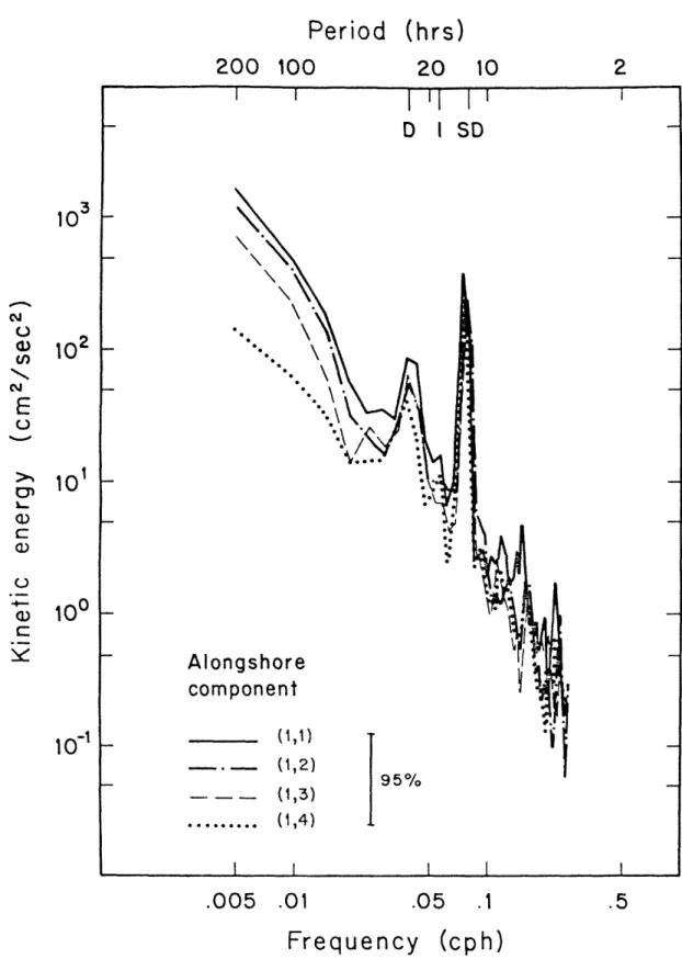
Figure 2.1 is an overlay of alongshore energy spectra at 4, 8, 12, and 18 m depths, located a distance of 3 km from shore. These results are typical examples of alongshore component spectra. The dominance of the SD peak and the general red character are clear. The low frequency energy varies roughly as -2, a value which is quite representative of results at differing offshore positions during the various experimental periods. While the energy reduction with depth shown here is quite

substantial (as high as an order of magnitude) it is more often found that the percentage of energy decrease with depth is not a strong function of frequency for SD and longer period oscillations. High

frequency motions in this figure and in general are relatively depth independent, and in fact are statistically isotropic.

Period (hrs)

200

100

--

__

(1,3)

.005

.01

20

10

Frequency

Figure 2.1 Aug '78 alongshore kinetic energy spectra 3km from shore at depths of 4,8,12, and 18 m. I I

2

102

10

U

N

E

0

a)

.E

Alon

com

.5

(cph)

\ N

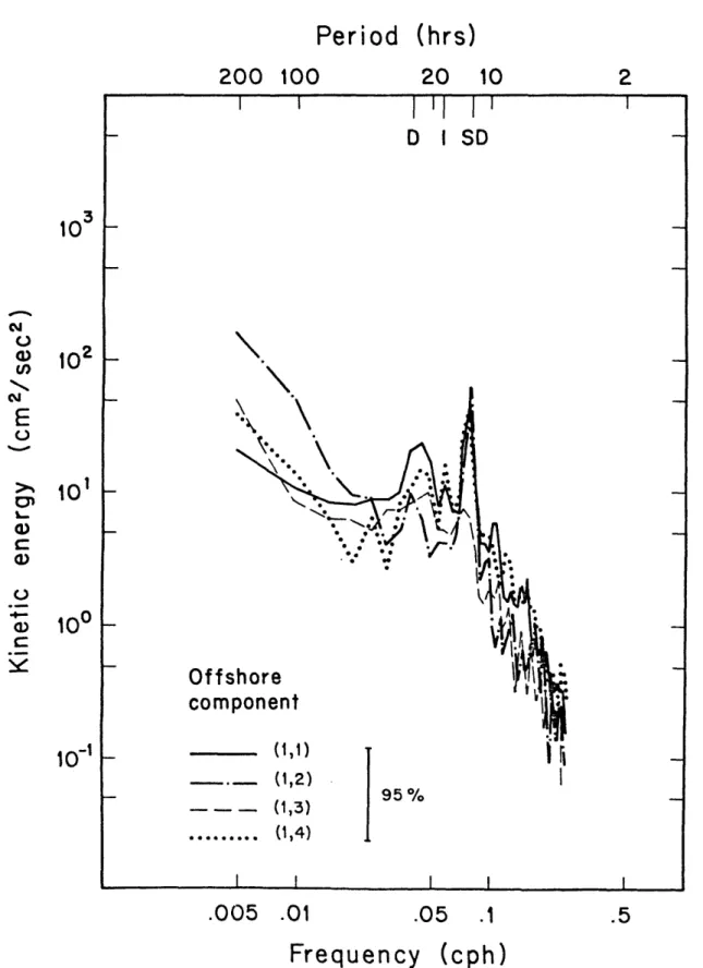
Figure 2.2 shows the corresponding offshore energy levels. The fact that the variation with depth is not as orderly as for the alongshore component is probably at least partly due to the inherent difficulty

associated with measuring the cross-shore component of low frequency motions which are highly polarized in the alongshore direction. It is easily appreciated that small angular deviations in current meter ori-entations could lead to significant contamination of relatively weak

cross-isobath signals. In addition to this difficulty, the presence of the coastal boundary may also be expected to contribute to the vertical variability of offshore velocity components because of the general ten-dency of the nearshore water column to conserve mass through a two dimensional transverse circulation pattern. Despite these additional complications, several observational facts are clear. Energy levels in SD and lower frequencies are significantly reduced relative to along-shore values, and the magnitude of that reduction increases with decreasing frequency. For the lowest frequencies resolved in this study, alongshore to cross-shore energy ratios of order 10 are fre-quently observed. Energy levels of the higher frequencies (greater than SD) are statistically indistinguishable from their alongshore counter-parts.

2.2 Cross-shore variation of energy

cross-Period (hrs)

200

100

20

10

Offs

comI

--

_

(1,3)

...

(1,4)

I

.005 .01

.

Frequency

Figure 2.2 Aug '78 offshore kinetic energy spectra depths of 4, 8, 12, and 18 m. 3 km from shore at

2

102

101

0

_a

01

0

.5

(cph)

shore structure of the CBL it might be expected that energy spectra would be strong functions of the offshore coordinate. In point of fact, however, there is little compelling evidence of this type of behavior except in a few notable cases.

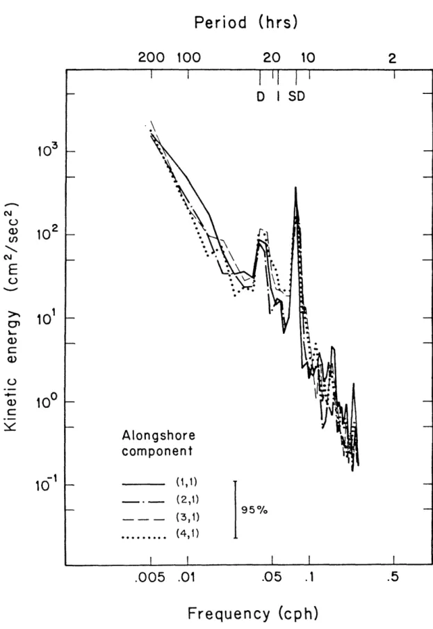
Figure 2.3 illustrates the alongshore energies 4 m below mean sea level at each mooring in the August 1978 experiment. There is some indication here of a monotonic shoreward amplification of the SD tidal velocities at this level. This type of behavior has been previously noted by (among others) Flagg (1977) and Smith et al. (1978) in their respective studies of the New England and Scotian shelves. In the coastal boundary layer, however, this trend is reversed with depth as the effect of friction apparently becomes more important than shoaling. The overall result is that no significant cross-shore variation for SD currents is observed.

Subtidal energy levels show an interesting behavior as the coastline is approached. It may be noted in Figure 2.3 that a statistically insignificant rise in low frequency alongshore energy occurs at mooring 1 located 3 km from shore. The fact that this behavior is noted at all vertical positions and in both the March and August experiments (the only experiments which included a functional mooring at this position) gives some credence to the notion that this may be a characteristic, albeit somewhat subtle, pattern. If the existence of shoreward ampli-fication of low frequency energy levels were accepted it would have several important implications. First, it would indicate that simple linear theories of coastally trapped shelf waves and quasi-steady

Period (hrs)

200

100

20

10

Alon

comI

...

(4,1)

I

.005

.01

.05

Frequency (cph)

Figure 2.3 Aug '78 alongshore kinetic energy spectra at 4 m depth, 3, 6, 9, and 12 km from shore.

2

o

a)

c

E

0

L.

0

102

100

.5

very shallow water only a few km from shore. In addition, since the region of strong topographic variation in the COBOLT study area is

shoreward of 5 km i.e., in the same region in which the low frequency

amplification seems to occur, it seems likely that consideration of nearshore details of bottom topography would be a key factor influencing cross-shore variability in the CBL.

Not surprisingly, offshore component energy spectra show more clear variations with the cross-shore coordinate. As seen in Figure 2.4 there is a significant decrease in energy between buoys 1 and 4 for subtidal frequencies. This is a "robust" result in that it is evident during all experimental deployments.

Up until this point, spectra shown have been exclusively from the August 1978 experiment because it represents the most complete data set

in terms of space-time coverage and instrument performance. Neverthe-less, important complementary information about seasonal and intermit-tent phenomena is available from the other COBOLT deployments. As the reader has doubtless discovered, no significant peaks of inertial fre-quency appear at any location throughout the August experiment. This

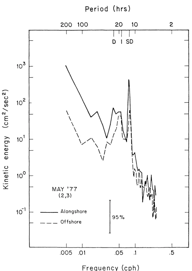
lack of inertial energy is not surprising given the weak (generally less

than 0.5 dyne) wind stress during the period, as well as the shallowness of the water column and the proximity of the shoreline. In contrast, the May 1977 experiment showed strong inertial energy as close as 6 km from the coast in water roughly 25 m deep.

Figure 2.5 is an example of offshore and alongshore kinetic energy spectra which show significant inertial peaks occurring at 16 m depth,

Period (hrs)

200 100

20

10

Offs

comr

...

(4,1)

.005

.01

Frequency

Figure 2.4 Aug '78 offshore kinetic energy spectra at 4 m depth, 3, 6, 9, and 12 km from shore.

2

E

C-10

10

ib-'

.5

(cph)

Period (hrs)

200 100

20

10

7/

I,;.

Frequency

(cph)

Figure 2.5 May '77 alongshore and offshore spectral energies at 8 m depth, 6 km from shore.

2

E

0

a)

102

lo1

10

(2

.5

6 km from shore. The inertial energies from the alongshore and offshore signals are seen to be essentially equal (as they must be for an iner-tial balance) and are comparable to the alongshore diurnal and offshore semidiurnal tidal energy levels. In fact, near-surface inertial ener-gies were observed to dominate the offshore energy spectra. In Figure 2.5 the inertial and diurnal frequencies are contained within one broad lobe and it is important to make a case for contributions from two dis-tinct physical forcing mechanisms rather than, as might be imagined, spectral leakage or frequency shifting of diurnal energy resulting in a broad band of essentially tidal origin. One bit of evidence against the notion that the near-inertial energy observed in May '77 was the result of frequncy shifting of diurnal motions, is the fact that during Aug

'78, when conditions were actually more conducive to this process, energy in the inertial band was notably absent. In addition, a clear

distinction between inertial oscillations and those of tidal frequency is easily demonstrated through calculation of the so-called rotary spectrum (Gonella, 1972).

2.3 The rotary-spectral description

The rotary component method of data analysis is based upon the fact that any orthogonal pair of velocities u and v which are periodic with frequency may be expressed as

iwt

-iwt

(2.1)

where Aa and Ac are complex amplitudes. This formulation in

effect represents the combination of two vectors which rotate in an opposite sense so that the velocity signal at a given frequency may be thought of as consisting of both clockwise and anti-clockwise portions. An arbitrary complex time series may be represented by the summation over frequency of equation (2.1). The two sets of complex coefficients resulting from such a Fourier decomposition may be used to compute clockwise-and anti-clockwise energy spectra as shown below.

Sc(w) = 1/2 Ac(W)A c()*

(2.2) Sa () = 1/2 I Aa(W)Aa(W)*

where the * superscript represents complex conjugation. The total spectrum is given by

ST(W) = Sc(W) + Sa( ) (2.3)

The foregoing relations are, of course, invariant under coordinate rotations.

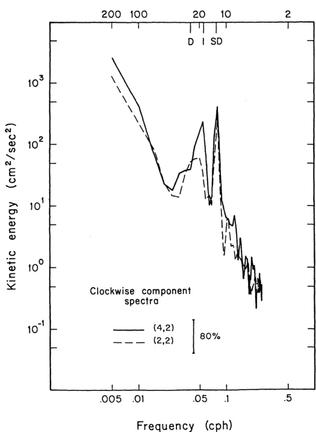
Inertial motions are dynamically constrained (in the northern hemisphere) to be clockwise circular motions and as such should be distinguishable from leakage and other contamination from adjacent

peaks. Figure 2.6 shows the clockwise and anti-clockwise energy spectra corresponding to the previous illustration. There is an unambiguous

dicotomy between the structures at diurnal and inertial frequencies. A two order of magnitude discrepancy in clockwise versus anti-clockwise

energy exists near inertial frequency which indicates a nearly perfectly circular clockwise motion. In contrast, the diurnal signal while still

predominantly clockwise contains relatively high anti-clockwise energy as well, giving rise to a motion which is elliptic in character.

The eccentricity, sense of rotation, and ellipse orientation for these, and all frequencies of interest, are easily quantified within the framework of rotary component analysis (Gonella, 1972). The "rotary coefficient" whose value ranges between +1 is defined as

R(w) = ( Sc() - Sa(m) )/ ST() (2.4)

and tells a great deal about the character of the motion. By inspection it is seen that for predominantly clockwise signals R > O, while R < 0 for anti-clockwise motions. In the cases of purely clockwise or anti-clockwise oscillation, the values are 1 and -1 respectively. When the two components are equal, that is for unidirectional (nonrotational) conditions, R = O. In essence, the sign of the rotary coefficient des-cribes the direction of rotation and its magnitude is indicative of the relative ellipticity of the motion. In fact, the rotary coefficient may be related to the more familiar eccentricity of the ellipse by

Period (hrs)

200 100

20

10

.005

.01

Frequency

)5

.1

.5

(cp.h)

May '77 rotary spectral components at 8 m depth, 6 km from shore.

2

E

L.

.0

102

101

100

101

e = 1 - IRI (2.5)

For the case corresponding to Figure 2.6, the rotary coefficients for inertial and diurnal frequency are .96 and .56 indicating respec-tively one circular clockwise motion and a tidal ellipse of eccentricity 0.44.

The rotary coefficient presents a compact representation of the rot-ational aspects of the flow field. From a compilation of this coeffi-cient for the entire COBOLT program the following general observations can be made:

(1) Low frequency (8 day) motions are essentially rectilinear in nature.

(2) Motions in the 2-4 day band display a general tendency to rotate anti-clockwise near surface and clockwise near bottom.

(3) Diurnal motions are clockwise at all depths.

(4) SD tidal currents rotate clockwise except near bottom where they often reverse their rotational direction.

(5) SD and inertial period motion becomes progressively more eccentric as the bottom is approached. Subinertial eccentricities reveal no clear pattern of vertical variation.

(6) There is no clear pattern to the horizontal variations of eccentricity.

TABLE 2.1

May '77 and Mar. '78 Rotary Coefficients

May '77 50.0 25.0 18.2 -.02 -.05 .36 -.49 -.12 -. 57 .08 .62 .59 .38 .56 .18 .73 .14 .58 .73 .91 .75 .96 .83 .98 .99 .95 .83 12.5 (hrs) .50 .28 .29 -. 26 .35 .43 .38 .24 Mar. '78 -.22 -.12 .04 .15 .46 -. 04 .38 .64 .28 .11 .40 .57 .11 .26 .62 .12 .66 .90 .60 .08 .99 .97

.62

TABLE 2.2

Aug.'78 Rotary Coefficients

periods 67.7 25.0 -. 06 .08 .12 .30 -. 11 .07 .41 .56 -. 01 -. 04 .08 .16 .15 .00 .23 .15 .43 .01 .13 .11 .52 .23 .06 -. 30 .58 .38 .26 .02 .71 .31 .46 .17 12.5 (hrs) .53 .39 .18 -. 21 .19 .25 .74 -.05 .02 .22 .53 .35 .14 .39 .56 .30 Inst. no. (1,1) (1,2) (1,3) (1,4) (2,1) (2,2) (2,3) (2,4) (3,1) (3,2) (3,3) (3,4) (4,1) (4,2) (4,3) (4,4) 200.0 .02 .03 .09 -.06 -.07 .01 -.07 .06 -. 27 -. 20 .00 .14 -. 35 -. 31 -. 24 .14

2.4 The vertical structure of fluctuating currents

The spatial relationships between fluctuating geophysical variables are often key factors in the understanding of regional dynamics. His-torically the unraveling of these relationships has proved somewhat tractable through the application of cross-spectral analysis and methods of empirical orthogonal modal analysis. In the general case where more than one type of "wave" structure is present in the same frequency band, there is considerable ambiguity in the interpretation of cross-spectral relationships. In particular, as'discussed by Wallace (1971), there is no way to clearly distinguish between independent processes nor to dis-cover their relative contribution to the overall signal. Because of these shortcomings a group of procedures called empirical orthogonal methods (EOMs) have evolved. The basic unifying theme in all such met-hods is the calculation of a set of eigenvectors, each corresponding to a specified fraction of the total energy, which form a linearly indepen-dent basis set in terms of which the observations may be expressed.

The EOM in most common usage involves finding the eigenvectors of the covariance matrix. If one is interested in several frequency bands this procedure becomes cumbersome as it requires making the calculation for various bandpassed versions of the data set. However, as shown by Wallace and Dickinson (1972) one can transform to the frequency domain

and calculate the complex eigenvectors of the cross-spectral matrix which, in addition to properties analogous to those of the covariance matrix, contain phase information. Due to the fact that the thrust of

Wallace and Dickinson's work was aimed at the generation of real valued time series corresponding to the independent complex eigenmodes present in observations, the method entails additional complications involving transformation of "augmented" time series; a combination of the original series and their time derivatives. These added complexities are unnec-essary, however, if one's principal interest is only the spatial and phase structures of the empirical modes. In this case the complex eig-envectors themselves directly give the amplitude and phase as a function of position, and the associated eigenvalues reveal how much energy is associated with each eigenvector or empirical mode. The advantages of this method are that once the appropriate cross-spectra have been calcu-lated one has merely to perform the numerical diagonalization of the complex hermitian matrix for any frequency of interest in order to obtain the vertical or horizontal modes.

Operationally the calculations performed in the present study went as follows. Cross-spectra were computed for all possible combinations of current meters on a given mooring. Then for any frequecy band of interest over which significant coherence levels were obtained for all current meter pairs, the hermitian cross-spectral matrix was formed as

All C1 2 + iQ1 2 C1 3 + iQ1 3 C1 4 + iQ1 4

C1 2 - iQ1 2 A2 2 C2 3 + iQ2 3 C2 4 + iQ2 4

C1 3 - iQ1 3 C2 3 - iQ2 3 A33C 3 4 iQ3 4

where Aii are the various autospectra and Cij and Qij are the cospectra and quadrature spectra between the ith and jth instruments. This matrix was then diagonalized by a standard "canned" computer routine yielding the 4 real eigenvalues and their associated complex eigenvectors. Since the trace of the matrix is invariant, the sum of the eigenvalues equals the total energy and is conserved. The amount of the total variance contained in each eigenmode is determined by the proportion of its

associated eigenvalue relative to the trace. The modes are subsequently ranked according to energy content and the modal structure determined from the moduli and phases of the complex elements of the eigenvector.

For presentation the amplitudes were scaled by the maximum value within each mode and the relative phase of the first element arbitrarily set equal to zero. Horizontal or crossshore modes may be calculated in an exactly analogous manner. The preceding methodology was brought to the

author's attention by Dr. N. G. Hogg and was employed in Hogg and Schmitz (1981).

The question of whether the structures emergent from the empirical orthogonal function analyses represent bona fide physical processes, statistical artifices, or manifestations of random noise needs some consideration. Wallace and Dickinson (1972) suggest that a ratio of at least 2:1 in successive eigenvalues (variances) is fair assurance of statisical significance. Hogg and Schmitz point out that this ratio is approximately the 95 percent confidence level below which successive eigenvalues and thus eigenfunctions are indistinguishable from white noise with 20 degrees of freedom. Unfortunately assurance of the

statistical significance of the modes is necessary but insufficient assurance of their physical significance. From a pragmatic point of view, the first several eigenvectors in the expansion are merely the linear combination which most efficiently reconstruct the structure of the cross spectral matrix. In this light it is seen that the empirical mode analysis is most useful when the structures found are consistent with some recognized physical conceptualization of the system being studied.

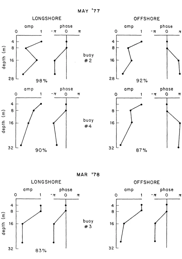
Representative illustrations of the amplitude and phase structures of vertical empirical eigenmodes of low frequency (.005), tidal fre-quency, and inertial frequency bands are presented in figures 2.7 and 2.8. Large vertical shears were found to be associated with the domi-nant alongshore modes calculated for all moorings during all experi-ments. The fact that the motions are essentially in phase at all depths (except for inertial frequency modes) suggests a barotropic interpre-tation. The vertical shears observed are likely to have been friction-ally induced and underscore the importance of frictional influences in this shallow region. This view is further supported by the slight but consistently observed near bottom phase shifts. The low frequency and SD signals consist almost entirely of these frictional barotropic modes in the March and May experiments, while in August there is evidence of well defined though relatively weak secondary mode as well (present only at 200 hours in figure 2.7). These auxiliary modes, which account for approximately 3 percent of the total energy at this frequency, have a phase structure which closely resembles that of the internal response of

AUG '78 MODE 1 phase 1 -7r 0 LONGSHORE 7r BUOY # 1 MODE 2

amp

4

20

amp

phase

20

-

_99%

Low-frequency, diurnal, and semidiurnal

amp 0 4 8 12 E -c 0 20 phase -r 0 7r 7V/O _{~ 7o} 1 -1 _1. I

Fiqure 2.7

_{complex eigenmodes.}

I

MAY

'77

98%

#2

90%

#4

92%

MAR '78

83

83%

-Figure 2.8 Inertial frequency complex eiqenmodes. 0 4 8 16 E ,c ,,,,-4 8 16 E v C--0 C-0 4 8 16 E C 0), D 32 _ I 28 _ 'v

I

a two-layer fluid in that it exhibits a 1800 phase change with depth. In conjunction with this phase change the amplitude goes through a local minimum in accordance with what one would expect in association with the so-called first mode internal oscillation of a stratified fluid. In this sense the empirical modes may be loosely termed baroclinic. The SD motions are of uniform phase everywhere except at mooring 4 in Aug

'78 where an apparent first baroclinic mode contributes approximately 5 percent of observed variance.

Alongshore empirical orthogonal modes of diurnal period character-isically exhibited one or more auxiliary modes which at times accounted for as much as 15 percent of the energy at this frequency. The phase and amplitude structures of these modes were generally more complex than those previously discussed, and their relation to dynamical modes of a stratified fluid is not so apparent. Nevertheless, it seems justified to attribute this portion of the diurnal energy to internal tidal oscil-lations.

The most striking result of the empirical orthogonal function decom-position is the observed structure of the inertial period signals shown in figure 2.8. The dominant motions, for both offshore and alongshore components, exhibit a very clear 180 degree phase shift between the upper and lower pairs of current meters. Even at buoy 3 in March '78, where the inertial signal strength and the stratification are weak, this behavior is quite evident, and has the qualitative aspect of an internal or baroclinic response of a two layer fluid. So in effect, while at all other frequencies examined in this study the alongshore component motions

display a uniform phase structure, the inertial frequency response of the coastal boundary layer under conditions of both weak and strong stratification, is characterized by a very clear 180° phase change with depth. Although this phase structure of the inertial motion does owe

its existence in part to the presence of stratification, it will be

shown in Chapter III that it may not be quite appropriate to label it baroclinic in the usual sense of the terminology.

Vertical modes of the offshore velocity field generally tend to be more complex and to have greater spatial variation than their alongshore counterparts. In fact, only the SD signal consistently shows the con-stant phase reponse that typifies the (non-inertial) alongshore compon-ents. This situation may reflect the expected lower relative accuracy with which cross-shore signals are recorded and/or the also expected

increase in vertical structure due to the coastal boundary constraint. However, it may also be, as concluded by May (1979), that the internal motions make a relatively greater contribution to the cross-shore modes since the barotropic motions are strongly polarized in the alongshore direction.

INERTIAL CURRENTS IN THE COASTAL ZONE: OBSERVATION AND THEORY

3.1 Introduction

The appearance of significant inertial oscillations in the COBOLT data is believed to represent the first reported observation of inertial frequency motion within a shallow oceanic coastal boundary layer envi-ronment. Historically coastal observations of near-inertial oscilla-tions, such as those noted by Flagg (1977), and Mayer et al. (1980), have shown inertial kinetic energy to decay rapidly in the shoreward direction thereby limiting significant levels to middle and outer shelf

locations. Off the Oregon coast Hayes and Halpern (1976), and Kundu (1976) have reported substantial near-inertial energy within - 15 km of shore in relatively deep (order 100 m) water. The fact that these observations have been exclusively associated with conditions of strong stratification has supported the notion that, in shallow water, fric-tional dissipation very efficiently damps inertial motions unless they are effectively isolated from such effects by a sufficiently strong pyc-nocline (Mayer et al., 1979). This interpretation is also suggested by the numerical model of Krauss (1976a,b) which investigated the effects that depth dependent stratification and eddy viscosity had upon the generation of inertial motion. The observation that inertial energy

substantially decreases in the shoreward direction has generally been interpreted as a manifestation of increased frictional influence as the water column shoals (eg. Flagg, 1977).

In some respects, because of the lack of competition from tides, large lakes represent an ideal environment in which to study nearshore inertial oscillations. Malone (1968) and Smith (1972) measured

nearshore currents in Lake Michigan and Lake Superior respectively, and noted that near-inertial currents occurred only in the presence of a thermocline. Malone's measurements suggested that these oscillations, which often completely dominated current meter records, were first mode

internal waves in that they exhibited a phase difference of 1800 across the thermocline. Both investigators noted a dramatic reduction in rotary motion as the shoreline was approached, and attributed this

behavior to the increased influence of the coastal boundary condition. Blanton (1974) clearly demonstrated that in Lake Ontario a rapid

transition between the predominance of the near-inertial motions of the interior and the lower frequency longshore boundary flow took place within the first 10 km from shore.

The implications of both continental shelf and lake studies are that one might expect both bottom friction and the proximity of the shoreline to inhibit inertial motions within the oceanic CBL. It is also expected that this inhibition will become progressively greater as the coast is approached. Observational evidence also suggests that stratification plays a fundamental role in the realization of inertial motion in shelf regions and enclosed basins.

3.2 Wind stress and inertial currents

During the COBOLT experirlent wind speed and direction were recorded at various nearby towers under the auspices of BNL's Meteorology Group. In addition, wind profiles were recorded at the field site in a 1974 study relating local mean winds to bulk aerodynamic drag coefficients. SethuRaman and Raynor (1975) in an analysis of these data concluded that the drag coefficient was not discernably a function of wind speed. More recently, however, Amorocho and Devries (1979), using a large collection of data have presented an empirically determined formula for the drag coefficient as a function of wind speed. This formula is entirely consistent with, although not suggested by, the data of SethuRaman and Raynor which represented a limited range of observed wind speeds. In the present work the variable coefficient given by Amorocho and Devries as

C₁₀ = 0.0015 [ 1 + exp( 12.5 - U₁₀ ) ]-1 + 0.00104 (3.1) 1.56

is adopted, where C₁₀ is the coefficient relevant to mean flow at 10 meters (U1 0) in KS units. While one is never overly comfortable

relying on such bulk formulae, it is expected that use of Eq. (3.1) leads to a reasonable representation of wind stress fluctuations.

The idea that wind stress fluctuations are largely responsible for the generation of open ocean near-inertial motions is well founded on both theoretical (Gonella, 1970; Pollard, 1970; Krauss,1976a,b) and