HAL Id: hal-00304908
https://hal.archives-ouvertes.fr/hal-00304908
Submitted on 1 Jan 2003HAL is a multi-disciplinary open access archive for the deposit and dissemination of sci-entific research documents, whether they are pub-lished or not. The documents may come from teaching and research institutions in France or abroad, or from public or private research centers.
L’archive ouverte pluridisciplinaire HAL, est destinée au dépôt et à la diffusion de documents scientifiques de niveau recherche, publiés ou non, émanant des établissements d’enseignement et de recherche français ou étrangers, des laboratoires publics ou privés.
Assessing emission reduction targets with dynamic
models: deriving target load functions for use in
integrated assessment
A. Jenkins, B. J. Cosby, R. C. Ferrier, T. Larssen, M. Posch
To cite this version:
A. Jenkins, B. J. Cosby, R. C. Ferrier, T. Larssen, M. Posch. Assessing emission reduction targets with dynamic models: deriving target load functions for use in integrated assessment. Hydrology and Earth System Sciences Discussions, European Geosciences Union, 2003, 7 (4), pp.609-617. �hal-00304908�
Assessing emission reduction targets with dynamic models:
deriving target load functions for use in integrated assessment
A. Jenkins
1, B.J. Cosby
2, R.C. Ferrier
3, T. Larssen
4and M. Posch
51CEH Wallingford, Oxfordshire, OX10 8BB, UK
2Department of Environmental Sciences, University of Virginia, Charlottesville, VA22901, USA 3Macaulay Institute, Aberdeen, Scotland AB15 8QH, UK
4Norwegian Institute for Water Research, Box 173, N-0411 Oslo, Norway
5Coordination Center for Effects/RIVM, Box 1, NL-3720 BA Bilthoven, The Netherlands
Email for corresponding author: [email protected]
Abstract
International agreements to reduce the emission of acidifying sulphur (S) and nitrogen (N) compounds have been negotiated on the basis of an understanding of the link between acidification related changes in soil and surface water chemistry and terrestrial and aquatic biota. The quantification of this link is incorporated within the concept of critical loads. Critical loads are calculated using steady state models and give no indication of the time within which acidified ecosystems might be expected to recover. Dynamic models provide an opportunity to assess the timescale of recovery and can go further to provide outputs which can be used in future emission reduction strategies. In this respect, the Target Load Function (TLF) is proposed as a means of assessing the deposition load necessary to restore a damaged ecosystem to some pre-defined acceptable state by a certain time in the future. A target load represents the deposition of S and N in a pre-defined year (implementation year) for which the critical limit is achieved in a defined time (target year). A TLF is constructed using an appropriate dynamic model to determine the value of a chemical criterion at a given point in time given a temporal pattern of S and N deposition loads. A TLF requires information regarding: (i) the chemical criterion required to protect the chosen biological receptor (i.e. the critical limit); (ii) the year in which the critical limit is required to be achieved; and (iii) time pattern of future emission reductions. In addition, the TLF can be assessed for whole regions to incorporate the effect of these three essentially ecosystem management decisions.
Keywords: emission reduction, critical load, target load, dynamic model, recovery time
Introduction
The link between the emission of oxides of sulphur and nitrogen (and reduced nitrogen) to the atmosphere and the subsequent acidification of soils and surface waters is now well established and understood (Grennfelt et al., 1995). The impact of the acidification-related changes in soil and surface water chemistry on associated biota is also sufficiently understood such that chemical criteria (i.e. critical limits) can be specified for soils and surface waters for the protection of both aquatic (Jenkins et al., 2003) and terrestrial organisms (Sverdrup and Warfvinge, 1993). For ecosystems that have not yet been damaged by acidic deposition, these critical limits provide a measure of the
minimum environmental quality that must be maintained if future damage is to be avoided. For systems whose ecological function has been degraded by acidic deposition, these critical limits establish standards of environmental quality to guide and to assess the restoration of the ecosystem. By working backward along the causal chain from critical limits, through deposition and atmospheric transport and ultimately to the emissions sources, quantitative relationships between emissions and environmental response can be developed for many different ecosystems in large geographical areas. These relationships are crucial to the rational development of policy measures designed to reduce emissions to prevent or alleviate
A. Jenkins, B.J. Cosby, R.C. Ferrier, T. Larssen and M. Posch ecosystem acidification (Bull et al., 2001).
The quantitative links between emission of S and N compounds, their deposition, and biological effects have been formulated within the concepts of critical levels of pollutants and critical loads of deposition (e.g. Bull et al., 2001). The critical load is defined as a quantitative estimate of the exposure to one or more pollutants below which significant harmful effects on specified sensitive elements of the environment do not occur according to present knowledge (Nilsson and Grennfelt, 1988). The concept of critical load thus defined does not incorporate any measure of the time involved for emission reductions (and therefore deposition reductions) to be implemented, or of the time involved for ecosystem response. The critical load under consideration is essentially a steady state deposition load that does not exceed the long-term ability of the ecosystem to neutralise the potentially harmful effects. Thus, as long as other factors (such as climate or land use) do not change the ecosystem structure, there should be a unique value of critical load for each pollutant (or group of pollutants as in the case of acidic deposition) for each sensitive component within an ecosystem that represents the long-term sustainable response of that sensitive component to acidification.
Recent international agreements on emission reductions have been reached using the critical loads concept, mostly under the auspices of the 1979 UNECE Convention on Long-range Transboundary Air Pollution (LRTAP). European data bases and maps of critical loads have been instrumental in formulating effects-based Protocols to the LRTAP Convention, such as the 1994 Protocol on Further Reduction of Sulphur Emissions (the Oslo Protocol) and the 1999 Protocol to Abate Acidification, Eutrophication and Ground-level Ozone (the Gothenburg Protocol). Each Party to the Convention determined which sensitive ecosystem components within their jurisdiction would be used to establish the critical loads for their country. More recently, EU legislation on emission reductions has been introduced under the National Emission Ceilings Directive. Subsequent to the agreements and the reductions in deposition thereby produced, monitoring programmes have shown that ecosystem acidification effects have been partially mitigated in many areas (e.g. Stoddard et al., 1999, Evans et al., 2001). Despite these successes, however, acidification remains a problem in many sensitive areas even with the achieved deposition reductions (Jenkins et al., 2003). The same monitoring programmes that have documented the partial recovery in response to deposition reductions have also demonstrated that the recovery responses of many ecosystems can be delayed significantly following reductions in acid deposition.
In the cascade of events from the deposition of strong acids to the damage of key indicator organisms, many processes are time and/or resource dependent and, therefore, can introduce delays in response. Hydrological and biogeochemical processes in catchments can delay the chemical responses of runoff and surface waters. Biological processes and population dynamics in the surface waters can further delay the response of indicator organisms.
These delayed responses may vary considerably in magnitude from place to place but a general pattern of chemical and biological responses to changing deposition is expected that can be described in five stages (Fig. 1). In stage 1, deposition is below the critical load (and has never exceeded it), and the chemical and biological variables do not violate their respective criteria. As deposition increases above the critical load, there is a delay before the chemical and biological criteria are exceeded (stage 2) as the buffering capability of the catchment is slowly depleted. In stage 3, deposition is above the critical load and both the chemical and biological criteria are violated. Measures (emission/ deposition reductions) have to be taken to avoid further deterioration of the ecosystem status and/or to restore it to acceptable status. As deposition declines below the critical load (stage 4), there will be a time lag before the chemical and biological criteria return to acceptable values. In stage 5, the deposition is below the critical load and the chemical and biological criteria are no longer violated. This stage is similar to stage 1 (though not necessarily identical in terms of biology or chemistry) and only at this stage can the ecosystem be considered to have recovered. Stages 2 and 4 can each be further subdivided into sub-stages that separate the chemical and biological delays. Very often, due to the lack of operational biological response models, damage and recovery delay times refer only to chemical recovery and this is used as a surrogate for overall recovery.
The existence of these delays in recovery and concern for remediation of damaged resources may lead to political and social pressures to accelerate the recovery process. In other words, the relevant question may not be: What is the deposition load necessary to restore and sustain a damaged ecosystem in the long-term steady state? Rather, the important question may be: What is the deposition load necessary to restore a damaged ecosystem to an acceptable state by a certain time in the (near) future? Such a deposition load might depend crucially on the time-scale of recovery involved. For example, recovery to a given ecosystem condition within 10 years would most probably require a larger and more immediate deposition reduction than would recovery to the same endpoint in 20 years.
The explicit inclusion of estimates of the time-scale of ecosystem recovery into critical loads analyses would
provide decision-makers with a powerful tool for setting (or modifying) emission policy. The objective of this paper is to define and explain the concept of the target load
function, to describe how it can be derived from dynamic
models, and to provide a conceptual description of its use as a tool for incorporating information about the dynamics of ecosystem recovery into the integrated assessment methodology. The target load function can be applied to individual sites or to regional collections of sites in an integrated assessment framework. The discussion and illustrations in this paper concern surface waters but the concepts can equally well be applied to terrestrial ecosystems.
Beyond critical loads
In determining the critical loads used in negotiating the emission reduction agreements currently in effect, the static models considered only the long-term, steady state
condition. These static models provide no estimate of the time required to reach this state. Given the observed delays in ecosystem responses, two related questions arise for which the steady state models provide no answer: (a) When will ecosystems recover in response to the agreed emission reductions and (b) Are further deposition reductions necessary to achieve recovery within a given time? From a policy or management viewpoint, more detailed information regarding the timing and degree of recovery is desirable, i.e. how long will it take for policies agreed today to show a benefit and do further reductions need to be implemented? Dynamic models of acidification and recovery can be used to provide an estimate of the expected surface water chemistry in the future in response to the implementation of the existing emission reduction agreements (assessment of the impact of emission reductions) (Jenkins et al., 2003). They can also be used to assist in the calculation (optimisation) of further emission reductions that may be required for complete recovery (a necessary input to the
Fig. 1. Conceptual patterns of acid deposition effects on a lake chemical variable (ANC) and a corresponding biological response variable
(critical abundance of a fish species) during increasing and decreasing deposition. Criterion values for acceptable minimal levels of the chemical and biological variables are indicated as horizontal lines, along with the critical load of deposition that will produce these levels. The delays between the exceedence of the critical load (t1), the violation of the critical chemical criterion (t2), and the crossing of the critical biological response (t3) are indicated in grey shades, highlighting the Damage Delay Time (DDT). Similar delays in chemical and biological recovery during deposition reductions (t4, t5, and t6) define the Recovery Delay Time (RDT) of the system.
Stage 1 Stage 2 Stage 3 Stage 4 Stage 5
Acid deposition Critical Load Chemical response [ANC]lim Biological response crit. abundance time t1 t2 t3 t4 t5 t6 DDT RDT
A. Jenkins, B.J. Cosby, R.C. Ferrier, T. Larssen and M. Posch process of integrated assessment modelling). Four models have been identified as being widely used, documented and tested with respect to the requirements of the LRTAP Convention (Posch et al., 2003a, Posch and Reinds, in press) and which are simple enough to be applied on a regional scale; SAFE (Warfvinge et al. 1993), SMART (De Vries et
al., 1989) and MAGIC (Cosby et al., 1985, 2001).
The question of ecosystem response within a given time frame defines the concept of a target load, as opposed to the critical load. Critical loads depend only on the characteristics of the ecosystem and therefore have a uniquely defined value. Critical load values can be produced either by static models (steady state by default) or by dynamic models (run to steady state). Target loads are also based on the characteristics of the ecosystem (and are unique to each ecosystem in that respect). Target loads, however, may take on many different values depending on the timetables for deposition reduction and ecosystem recovery and, thus, are not unique for a given ecosystem. Because of their explicit dependence on time, target loads can be produced only by dynamic models.
Dynamic models are currently capable of assessing the implications of achieving the emission reductions agreed under the Gothenburg Protocol (Jenkins et al., 2003). They address the question of whether the current agreements suffice to allow recovery and prevent further acidification of surface waters within a given timeframe, and help to identify regions where further reductions might be required to achieve the specified chemical criteria by some specified time. Perhaps more importantly, dynamic models also permit the calculation of time-dependent target loads, thus providing resource managers and policy-makers with a tool,
based on state-of-science knowledge about ecosystem response, which allows consideration of economic, political, and social constraints on future actions and results.
Target Load Functions
Acidic deposition consists of both S and N compounds, and critical load estimates consider both. Because the acidifying effects of S and N are similar in both aquatic and terrestrial ecosystems, it has become the accepted procedure when calculating critical loads to account explicitly for both components of acidic deposition by calculating the critical load function (Posch et al., 2003b).
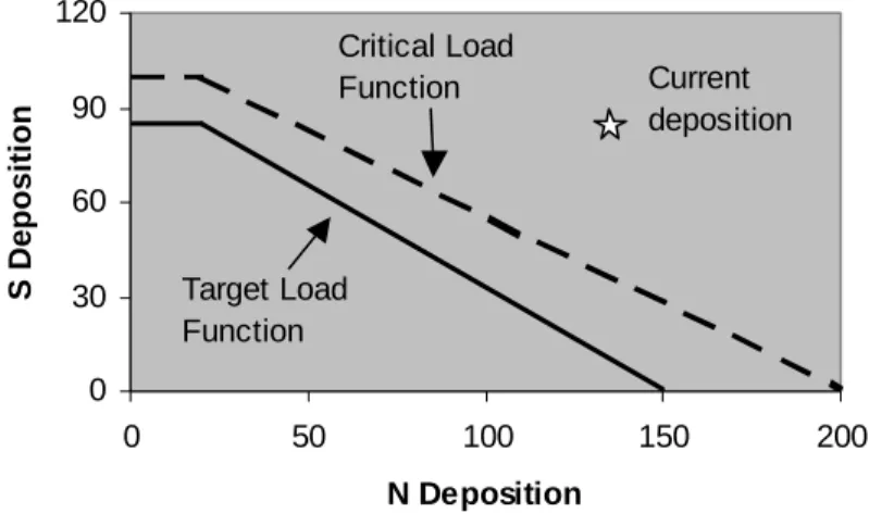
A Critical Load Function (CLF) is usually represented as a line of constant ecosystem response plotted on an x-y plane defined by S and N deposition values (Fig. 2). The lines generally have negative slopes because the amount of S deposition that can be sustained without violating biological or chemical criteria will in general be larger as N deposition is smaller (and conversely). The line is constructed by using the appropriate steady-state critical load model to determine the critical loads for many pairs of S and N depositions. These points are plotted on the x-y plane and intermediate points are interpolated.
The CLF is particularly useful in the integrated assessment process because it defines a continuous ecosystem response function that allows optimisation of emission controls within the constraint of the selected ecosystem protection criterion. For instance, if current deposition of S and N lies above the CLF when plotted in the x-y response plane, then the critical loads are exceeded, and ecosystem damage is expected at some time in the future (Fig. 2). The policy decision is to
Fig. 2. Example of a critical load function and target load function with respect to S and N deposition (meq m-2 yr-1) for a hypothetical ecosystem. Such functions are used by the integrated assessment models for calculation of optimal deposition reduction scenarios. Emission reductions must be achieved at some future time to achieve the target chemistry (critical limit) at some (unknown) point in the future. The target load function requires specification of the timing of emission reductions to achieve the critical limit in a given year.
0 30 60 90 120 0 50 100 150 200 N Deposition S De pos it ion Current deposition Critical Load Function Target Load Function
reduce S and/or N deposition until the new deposition falls on or below the CLF. There are, of course, many combinations of S and/or N deposition reductions that can accomplish this. The advantage of the CLF is that all of these possible solutions are included implicitly in the CLF. Decision makers use the CLF to choose the optimal emission reduction scenario based on analyses of economic, societal and political considerations, with the assurance that the desired ecosystem protection will be achieved.
A Target Load Function (TLF) is constructed in a manner similar to that of a CLF, with the important difference that time scales of deposition reductions and ecosystem change are included. As with the CLF, the TLF is represented as an isoline of ecosystem response plotted on an x-y plane defined by S and N deposition values (Fig. 2). The TLF is constructed by using the appropriate dynamic response model to determine the value of the critical limit at a given
point in time given an assumed temporal pattern of S and N
deposition changes for many pairs of S and N depositions. These points are plotted on the x-y plane and intermediate points are interpolated. The shapes of both the CLF and TLF are similar (Fig. 2), and both functions have a negative slope. The shelf at low N deposition in both the CLF and TLF represents the long-term sustainable capability of the system to utilise N. The prominence of this feature may vary between ecosystems (even being absent in some cases). In general, a TLF will plot below the CLF for a given ecosystem and response variable (Fig. 2) because attainment of a required ecosystem criterion within a finite time (the TLF) will generally require a larger (and more immediate) reduction in deposition than that required for a steady state ecosystem response (the CLF). In the limit, as the time scales selected for the TLF become very large (approach to steady state), the TLF and CLF will converge.
The TLF is useful in the integrated assessment process, and provides policy analysts with a continuous response surface which can be used to optimise emission reduction scenarios for S and N while ensuring that the specified degree of ecosystem protection will be achieved and given economic constraints. The TLF has the additional utility that the cost or benefit of requiring ecosystem recovery within a
given time frame can also be evaluated. The additional
reduction in deposition required to move from the CLF to the TLF (Fig. 2) is a measure of the additional cost of achieving the desired ecosystem recovery within the
specified time. This extra information, not available from
the CLF, can also be used in selecting the optimal emission control scenario and may be useful in reconciling political, societal and economic considerations.
The comparison of the TLF and CLF was presented from the case in which current deposition exceeds the CLF (and
therefore also the TLF; Fig. 2); this usually motivates the decision to modify emissions. In the case where the current deposition of S and N lies below the CLF, a different relationship exists between the CLF and TLF. If current deposition of S and N is below the CLF, the management implication is that S and/or N deposition can be increased (up to the CLF) without adverse effects to the ecosystem (at least with respect to the criterion being considered) provided the critical limit is not violated. In this case, the TLF would lie above the CLF. The reason for this change in relative location of the TLF is that the CLF marks the long-term sustainable deposition for the ecosystem and, if a finite time scale is added (i.e. ecosystem protection is required only for a finite length of time rather than for continuous sustainability), the amount of deposition to move the ecosystem to the brink of acceptability will be larger. That is, higher acid loadings can be sustained for shorter periods of time due to the delay between deposition and ecosystem damage (see Fig. 1). It is not anticipated or recommended, however, that TLFs be used in this case. If the current S and N deposition in an ecosystem does not exceed the CLF, then the CLF should be used by the decision maker in the emission optimisation analysis. For ecosystems not yet damaged, the long-term sustainable deposition loads should be the relevant endpoint of the policy.
Properties of Target Load Functions
Unlike the CLF, a unique TLF does not exist for a given ecosystem. TLFs depend on many properties, some of which are characteristic of the ecosystem and some of which are specified by management or policy considerations. The ecosystem characteristics are the same for all TLFs at a site; the management/policy considerations may not be. The time required to implement emissions reductions, the time allowed for ecosystem recovery, and the degree of ecosystem recovery (in terms of the chemical and /or biological criterion to be achieved) are all properties or characteristics of a TLF that must be specified before the TLF can be constructed. Thus, for a given ecosystem, multiple TLFs will exist which depend on the a priori specifications of these management/policy alternatives. TLFs can thus be thought of as dynamic functions, conditioned by a number of dynamic properties that define extended degrees of freedom not present in a CLF. These extended degrees of freedom make the TLF more adaptable and useful than the CLF in the context of integrated assessment activities.
TIME TO ACHIEVE THE CRITICAL LIMIT
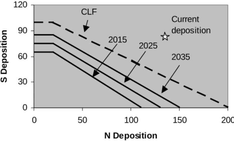
A. Jenkins, B.J. Cosby, R.C. Ferrier, T. Larssen and M. Posch achievement of the desired ecosystem response, the so-called target year. The location of the TLF in the S and N deposition space will be dependent on the required time in the future by which the critical limit must be achieved. Clearly, for most damaged ecosystems, recovery to the critical limit in 10 years will require greater reductions in deposition (and hence emissions) than recovery to the same criterion in 30 years (Fig. 3).
When passed to the policy analyst as part of an integrated assessment, such multiple TLFs offer two kinds of information. Firstly, by examining the relative position of the multiple TLFs, the analyst can determine the additional cost (in terms of greater emission reductions) incurred by requiring that ecosystem recovery be completed earlier rather than later. Conversely, if the emissions reduction optimisation methodology determines that S and N reductions must be limited to certain values (because of political, economic or other considerations), the position of the optimal deposition can be compared to the multiple TLFs, and the expected time it will take for the optimal emissions reduction scenario to produce the desired ecosystem recovery can be determined.
In general, the more quickly ecosystem recovery is desired, the lower the TLF relative to the CLF (Fig. 3). In the limit when very rapid recovery is sought, the TLF may move off the graph to zero indicating that the target is not achievable. For ecosystems that have been damaged, a finite period of time is always necessary for recovery. Even if deposition is reduced to zero, recovery will be limited by the biogeochemical characteristics of the ecosystem and may not occur for a number of years. It is in this aspect of integrated assessment (estimation of minimum recovery times) that the utility of dynamic, relative to static, models is most obvious.
TIMING OF DEPOSITION REDUCTION
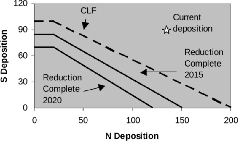
The implementation of a TLF analysis requires a priori decisions concerning the pattern of deposition reduction over time. As a simple example, the start and end years of the required reductions may be specified along with the assumption that deposition reduction will be linear in between. In this case, delay in either the beginning of emission reduction or the time period over which they are achieved will affect the position of the TLF (Fig. 4). In general, the longer the delay in implementing the emission reductions and/or the longer that is taken to complete the emissions reductions once begun, the lower will be the TLF relative to the CLF. Delay in implementing or completing reductions in emissions cause continuing stress on the ecosystem, such that when reductions are finally implemented they must be greater to achieve the desired ecosystem response in the required period of time.
This dynamic property of the TLF offers information of a slightly different nature to the analyst in an integrated assessment. Among the many political and economic considerations in developing an optimal emissions control strategy are the timing and rate of implementation of reductions in emissions. The protocol can usually provide upper and lower limits of how soon the proposed reductions would start to occur (protocol year) and how soon the reductions would be completed (the implementation year). Multiple TLFs could then be generated for a given ecosystem recovery criterion (and target date) that reflect the different control options under consideration. By analysing the position of the optimal deposition scenario in the S and N deposition space, the analyst can determine the additional costs (in terms of greater final emissions reductions required) that will be incurred by delaying the protocol or implementation years.
Fig. 3. The effect of different target years on the TLF at an individual site. 0 30 60 90 120 0 50 100 150 200 N Deposition S D e posit ion Current deposition CLF 2015 2025 2035
Regionalisation of Target Load
Functions
Decisions in an integrated assessment framework are usually based on a regional analysis of a group of ecosystems. These regional analyses provide decision makers with information about the extent of ecosystem recovery or protection (usually the number or percentage of sites) achieved under the proposed emission reduction protocols. These quantitative estimates of the extent of recovery in a region provide information for the development of optimal emission control strategies. In that these numerical measures of extent of protection are quasi-continuous (from 100% recovery to 0% recovery, for example), decision makers can compare the costs or benefits (in terms of ecosystems recovered) of alternate emission control scenarios. This concept has already been adopted for critical loads (Posch et al., 1995) and was used in the context of the Gothenburg Protocol.
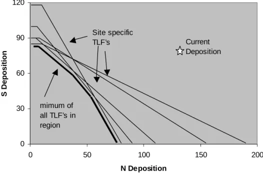
The TLF concept is easily extended from a specific site to a region. If data are available for a group of sites within a region such that an appropriate dynamic model can be calibrated for each site, then a TLF or series of TLFs can be developed for each site. Once the TLFs are available for each site, they can all be plotted on the same S and N deposition space (Fig. 5). Techniques (either quantitative or qualitative) can be used to plot a regional target load
function that defines the deposition space above or below
which some fraction of the regional site specific TLFs are located. Thus, in the simplest case, if recovery or protection is required for 100% of the sites, the regional TLF would be a line lying below all the site specific TLFs as shown in Fig. 5. Using this regional TLF to determine an optimal deposition scenario for S and N would ensure that the TLFs of none of the individual sites would be exceeded by the selected optimal scenario.
By extension, regional TLFs could be constructed for the recovery or protection of 95%, 90%, etc. of the regional resources. In general, the higher the percentage of regional resources protected, the lower the regional TLF curve will be. By comparing the regional TLFs for different levels of resource protection, policy analysts could determine the additional costs (in terms of additional emission reductions) required to extend protection to a larger percentage of the regional resource. Conversely, given an optimal emissions control scenario developed by consideration of economic, societal, and/or political constraints, the multiple regional TLFs can be used to specify the extent of ecosystem protection provided by that scenario.
Conclusions
The use of TLFs (Target Load Functions) in integrated assessment modelling of ecosystem response to acidic deposition provides a flexible tool that allows the explicit inclusion of emission reduction timetables and ecosystem response time in the decision making process. The TLF provides information that can be related to the costs and benefits of the degree of ecosystem recovery, the timing of ecosystem recovery and the timing of emission control protocols. In terms of achieving an optimal solution to emission reduction, the TLF can assist the policy maker in making key decisions regarding: (i) the year in which the critical limit is met (target year); (ii) the year in which emission reductions will need to be started (protocol year); and (iii) the year in which the emission reduction must be completed (implementation year). In addition, the TLF can be applied in a regional analysis that also incorporates the effects of these three control options. By developing multiple TLFs representing the range of possible values in each of
Fig. 4. The effect of different years of implementation of the emission reductions to meet the critical limit in 2025 at a
site. The two cases shown here represent the reductions beginning in 2010 and being completed by 2015 and 2020.
0 30 60 90 120 0 50 100 150 200 N Deposition S De pos it ion Current deposition CLF Reduction Complete 2020 Reduction Complete 2015
A. Jenkins, B.J. Cosby, R.C. Ferrier, T. Larssen and M. Posch
the control variables, it is possible to develop an optimal emission control strategy with respect to economic, political, and societal considerations that will provide the chosen level and timing of ecosystem recovery.
The development of TLFs for ecosystem responses requires the use of dynamic models. Dynamic model applications are, to a certain extent, limited by the availability of suitable data to describe the physico-chemical characteristics of surface waters and their terrestrial catchment areas. Dynamic model applications should first focus on areas that are already acidified or acid sensitive. This makes sense within the framework of the LRTAP Convention since emissions across Europe are declining and will continue to decline to year 2010 under the Gothenburg Protocol and so the speed of recovery from acidification is the key question.
Acknowledgements
This work was funded in part by the Commission of the European Communities (RECOVER:2010 Project EVK1-CT-1999-00018), the UK Natural Environment Research Council, the UK Department of the Environment, Food and Rural Affairs (Contract No. EPG 1/3/194), the Norwegian Pollution Control Authority, the Norwegian Institute for Water Research, and the Scottish Executive Environment and Rural Affairs Department.
Fig. 5. Calculation of a regional TLF. This would also represent a method for calculating the TLF within grid squares for a given target year.
References
Bull, K., Achermann, B., Bashkin, V., Chrast, R., Fenech, G., Forsius, M., Gregor, H-D., Guardans, R, Haussmann, T., Hayes, F., Hettelingh, J.-P., Johannessen, T., Krzyzanowski, M., Kucera, V., Kvaeven, B., Lorenz, M., Lundin, L., Mills, G., Posch, M., Skjelkvåle, B.L. and Ulstein, M.J., 2001. Co-ordinated effects monitoring and modelling for developing and supporting international air pollution control agreements. Water Air Soil
Pollut., 130, 119130.
Cosby, B.J., Hornberger, G.M., Galloway, J.N. and Wright, R.F., 1985. Modelling the effects of acid deposition: Assessment of a lumped parameter model of soil water and streamwater chemistry. Water Resour. Res., 21, 5163.
Cosby, B.J., Ferrier, R.C., Jenkins, A. and Wright, R.F., 2001. Modelling the effects of acid deposition: refinements, adjustments and inclusion of nitrogen dynamics in the MAGIC model. Hydrol. Earth Syst. Sci., 5, 499517.
De Vries, W., Posch, M. and Kämäri, J., 1989. Simulation of the long-term soil response to acid deposition in various buffer ranges. Water Air Soil Pollut., 48, 349390.
Evans, C.D., Cullen, J.M., Alewell, C., Kopácek, J., Marchetto, A., Moldan, F., Prechtel, A., Rogora, M., Veselý, J. and Wright, R.F., 2001. Recovery from acidification in European surface waters. Hydrol. Earth Syst. Sci., 5, 283297.
Grennfelt, P., Rodhe, H., Thornelof, E. and Wisniewski, J. (Eds.), 1995. Acid Reign 95? Water Air Soil Pollut., 85, 14. Jenkins, A., Camarero, L., Cosby, B.J., Ferrier, R.C., Forsius, M.,
Helliwell, R.C., Kopacek, J., Vajer, V., Moldan, F., Posch, M., Rogora, M., Schöpp, W. and Wright, R.F., 2003. A modelling assessment of acidification and recovery of European surface waters. Hydrol. Earth Sys. Sci., 7, 447455.
Nilsson, J. and Grennfelt, P., 1988. Critical loads for Sulphur and Nitrogen. Enviromental Report 1988, 15 (NORD 1988-97), Nordic Council of Ministers, Copenhagen, Denmark. 418pp.
0 30 60 90 120 0 50 100 150 200 N Deposition S De pos ition mimum of all TLF’s in region Site specific TLF’s Current Deposition
Posch, M., De Smet, P.A.M., Hettelingh, J-P., Downing, R.J. (Eds.), 1995. Calculation and mapping of critical thresholds in Europe: CCE Status Report 1995. RIVM Report 259101004, Bilthoven, The Netherlands. 198pp.
Posch, M. and Reinds, G.J., 2003. VSD User Manual of the Very
Simple Dynamic soil acidification model. Coordination Center
for Effects, National Institute for Public Health and the Environment (RIVM), Bilthoven, The Netherland (in press) . Posch, M., Hettelingh, J.P. and Slootweg, J., (Eds.), 2003a. Manual
for dynamic modeling of soil response to atmospheric deposition. RIVM Report 259101012, Bilthoven, The Netherlands. 69pp.
Posch, M. Hettelingh, J-P., Slootweg, J. and Downing, R.J., (Eds.), 2003b. Modelling and mapping of critical thresholds in Europe: CCE Status Report 2003. RIVM Report 259101013/
2003,Bilthoven, The Netherlands. 132pp.
Stoddard, J.L., Jeffries, D.S., Lükewille, A., Clair, T.A., Dillon, P.J., Driscoll, C.T., Forsius, M., Johannessen, M., Kahl, J.S., Kellogg, J.H., Kemp, A., Mannio, J., Monteith, D., Murdoch, P.S., Patrick, S., Rebsdorf, A., Skjelkvåle, B.L., Stainton, M.P., Traaen, T.S., van Dam, H., Webster, K.E., Wieting, J. and Wilander, A.,1999. Regional trends in aquatic recovery from acidification in North America and Europe 1980-95. Nature,
401, 575578.
Sverdrup, H. and Warfvinge, P., 1993. The effect of soil acidification on the growth of trees, grass and herbs as expressed by the (Ca+Mg_K)/Al ratio. Reports in Ecology and
Environmental Engineering, 2, Lund University, Lund, Sweden.
177pp.
Warfvinge, P., Falkengren-Grerup, U., Sverdrup, H. and Andersen, B., 1993. Modelling long-term cation supply in acidified forest stands. Environ. Pollut., 80, 209221.