https://doi.org/10.5194/essd-12-3039-2020 © Author(s) 2020. This work is distributed under the Creative Commons Attribution 4.0 License.
Worldwide version-controlled database
of glacier thickness observations
Ethan Welty1,2, Michael Zemp2, Francisco Navarro3, Matthias Huss4,5,6, Johannes J. Fürst7, Isabelle Gärtner-Roer2, Johannes Landmann2,4,5, Horst Machguth6,2, Kathrin Naegeli8,2,
Liss M. Andreassen9, Daniel Farinotti4,5, Huilin Li10, and GlaThiDa Contributors+ 1Institute of Arctic and Alpine Research (INSTAAR), University of Colorado, Boulder, USA
2World Glacier Monitoring Service (WGMS), University of Zürich, Zurich, Switzerland 3Escuela Técnica Superior de Ingenieros de Telecomunicación,
Universidad Politécnica de Madrid, Madrid, Spain
4Laboratory of Hydraulics, Hydrology and Glaciology (VAW), ETH Zürich, Zurich, Switzerland 5Swiss Federal Institute for Forest, Snow and Landscape Research (WSL), Birmensdorf, Switzerland
6Department of Geosciences, University of Fribourg, Fribourg, Switzerland 7Department of Geography, University of Erlangen–Nuremberg (FAU), Erlangen, Germany
8Institute of Geography, University of Bern, Bern, Switzerland 9Norwegian Water Resources and Energy Directorate (NVE), Oslo, Norway 10Cold and Arid Regions Environmental and Engineering Research Institute,
Chinese Academy of Sciences, Lanzhou, China +A full list of authors appears at the end of the paper. Correspondence:Ethan Welty ([email protected])
Received: 7 April 2020 – Discussion started: 27 May 2020
Revised: 1 September 2020 – Accepted: 6 October 2020 – Published: 24 November 2020
Abstract. Although worldwide inventories of glacier area have been coordinated internationally for several decades, a similar effort for glacier ice thicknesses was only initiated in 2013. Here, we present the third version of the Glacier Thickness Database (GlaThiDa v3), which includes 3 854 279 thickness measurements distributed over roughly 3000 glaciers worldwide. Overall, 14 % of global glacier area is now within 1 km of a thickness measurement (located on the same glacier) – a significant improvement over GlaThiDa v2, which covered only 6 % of global glacier area and only 1100 glaciers. Improvements in measurement coverage increase the robust-ness of numerical interpolations and model extrapolations, resulting in better estimates of regional to global glacier volumes and their potential contributions to sea-level rise.
In this paper, we summarize the sources and compilation of glacier thickness data and the spatial and tem-poral coverage of the resulting database. In addition, we detail our use of open-source metadata formats and software tools to describe the data, validate the data format and content against this metadata description, and track changes to the data following modern data management best practices. Archived versions of GlaThiDa are available from the World Glacier Monitoring Service (e.g., v3.1.0, from which this paper was generated: https://doi.org/10.5904/wgms-glathida-2020-10; GlaThiDa Consortium, 2020), while the development version is available on GitLab (https://gitlab.com/wgms/glathida, last access: 9 November 2020).
1 Introduction
A central challenge of glaciology is assessing the distribu-tion and total ice volume of the world’s glaciers. Increasingly detailed and globally complete inventories of the world’s glaciers (WGMS and NSIDC, 2012; GLIMS and NSIDC, 2018; RGI Consortium, 2017) have been compiled with great effort over the last few decades. However, these invento-ries have been limited to glacier extent and surface eleva-tion. The Glacier Thickness Database (GlaThiDa), launched by the World Glacier Monitoring Service (WGMS, https: //wgms.ch, last access: 9 November 2020) and supported by the International Association of Cryospheric Sciences (IACS) Working Group on Glacier Ice Thickness Estima-tion (https://cryosphericsciences.org/activities/ice-thickness, last access: 9 November 2020), complements these exist-ing efforts by compilexist-ing and publishexist-ing a freely accessi-ble database of glacier thickness observations (Gärtner-Roer et al., 2014).
Knowing the thickness of glacier ice is critical for predict-ing the rate and timpredict-ing of glacier retreat and disappearance, the subsequent effects on local and regional hydrologic cy-cles and global sea level, and the associated environmental and social impacts. As the only worldwide repository of its kind, GlaThiDa plays an important role in local, regional, and global studies of glaciers, glacier ice volumes, and their po-tential sea-level rise contributions (e.g., Thorlaksson, 2017; Farinotti et al., 2017, 2019; Meyer et al., 2018; Fischer, 2018; Ayala et al., 2019; Werder et al., 2020). The Ice Thick-ness Models Intercomparison eXperiment (ITMIX; Farinotti et al., 2017) only used GlaThiDa v1 (WGMS, 2014) to cal-ibrate one of the participating models, but it helped garner support and data for GlaThiDa v2 (WGMS, 2016). GlaThiDa v2 was subsequently used to calibrate all participating mod-els and evaluate model performance for an ensemble-based estimate of the thicknesses of all glaciers on Earth (Farinotti et al., 2019).
GlaThiDa v3 represents a major step forward for the database. We have more than doubled the spatial coverage and more than quadrupled the number of observations rel-ative to v2, released in 2016, adding 3 million thickness measurements either submitted by researchers (46 % of new measurements) or imported from the IceBridge Data Portal (54 %, https://nsidc.org/data/icebridge, last access: 28 Au-gust 2019). In addition to summarizing the spatial and tem-poral coverage of the database, we present a case study on how simple open-source metadata formats and software tools can be used to implement modern data management prac-tices. In the sections that follow, we describe a develop-ment environdevelop-ment for data – based on universal text-based file formats and the distributed version control system git (Chacon and Straub, 2014) – that maximizes data access and interoperability, automatically tracks and archives every change made to the dataset, continuously validates the struc-ture and contents of the data, and facilitates dialogue with
(and bug reports by) data users. A monospace font is used throughout the manuscript for software packages (e.g., git), files (e.g., datapackage.json), database tables (e.g., T), database table fields (e.g., POINT_LAT), and code samples (e.g., Fig. 3).
2 Methods and data 2.1 Data sources 2.1.1 Data compilation
Since the release of GlaThiDa v1 in 2014 (Gärtner-Roer et al., 2014), which focused on gathering glacier mean and maximum thickness estimates from published literature, a large number of thickness measurements have been submit-ted by members of the research community in response to two calls for data, one for version 2 in 2016 and another for version 3 in 2018. In all, researchers from institutions in Europe, North and South America, Oceania, and Asia have contributed data from Antarctica, Africa (Kenya, Tan-zania), Asia (China, Georgia, India, Kazakhstan, Kyrgyzs-tan, Mongolia, Nepal, Russia, Tajikistan), Europe (Austria, Germany, Greenland, Svalbard, Iceland, Italy, Norway, Swe-den, Switzerland), Oceania (New Zealand), North America (Canada, United States), and South America (Bolivia, Chile, Colombia, Peru).
Alongside these data submissions, airborne glacier thick-ness profiles collected by National Aeronautics and Space Administration (NASA) Operation IceBridge were retrieved from the corresponding National Snow and Ice Data Center (NSIDC) data portals. Since these campaigns were primar-ily focused on the Greenland and Antarctic ice sheets, only measurements within Randolph Glacier Inventory (RGI 6.0) glacier outlines (RGI Consortium, 2017) were included in GlaThiDa. These replaced the IceBridge data, located within Randolph Glacier Inventory (RGI 3.2) glacier outlines (RGI Consortium, 2013), included in GlaThiDa v1 in 2014.
2.1.2 Measurement methods
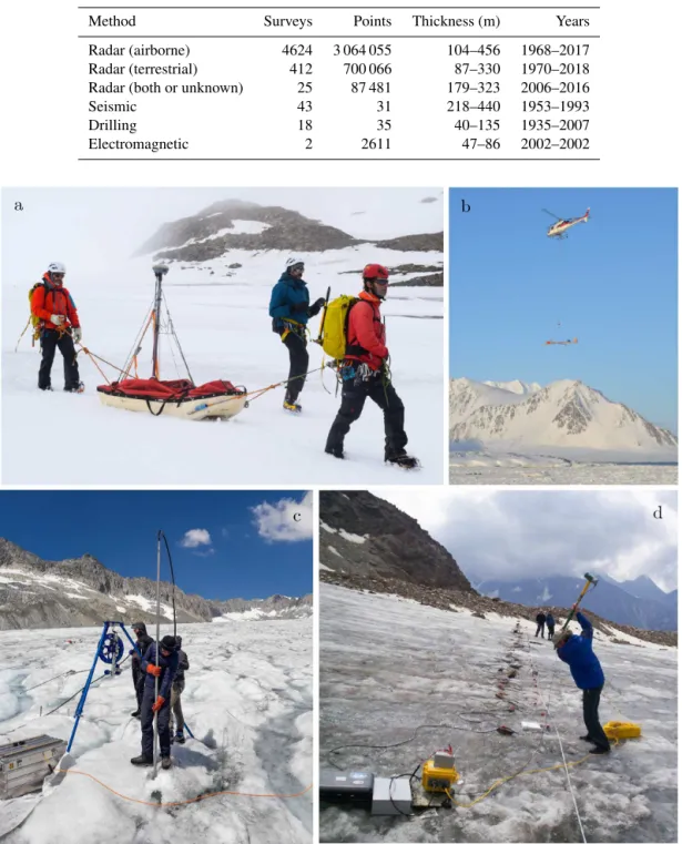
The surveys in GlaThiDa span the history of glacier ice thickness measurement and thus include several different survey methods, summarized in Table 1 and illustrated in Fig. 1. The most direct methods involve excavating or drilling through the ice. Although these typically produce a precise measurement, they do so only for a single point and at a great expense of time and money; correspondingly, these ac-count for only 0.35 % of surveys in GlaThiDa (here, a “sur-vey” roughly represents one measurement campaign on one glacier). The drilling surveys added in v3 (compiled by Fürst et al., 2018a, Table S3) were carried out in Svalbard in the 1970s through 1990s to map the thermal structure of glaciers (e.g., Jania et al., 1996) or to extract paleoclimate records (e.g., Kotlyakov et al., 2004). No drilling surveys were added in v2.
More often, ice thickness is measured indirectly using geo-physical methods. For example, seismic soundings employ the propagation properties of elastic waves to determine the structure of the subsurface (described in Susstrunk, 1951). Although common in the 1950s through 1980s, they are expensive and time-consuming to collect; correspondingly, these account for only 0.84 % of surveys in GlaThiDa. No seismic surveys were added in v3; of those already in the database, the majority were carried out in the Austrian Alps up until the 1970s (reviewed in Aric and Brückl, 2001). Only one seismic survey – of Tasman Glacier, New Zealand, from 1971 (Anderton, 1975) – was added in v2.
The most common geophysical method is radar (i.e., ra-dio detection and ranging, also known as “rara-dio-echo sound-ing” or “ground-penetrating radar”), which is based on the transmission, reflection, and subsequent detection of radio waves (reviewed in Schroeder et al., 2020). Radar mea-surements can be collected quickly, from the ice surface or from airborne platforms, and account for 98.44 % of sur-veys in GlaThiDa. Of the radar sursur-veys added in v3, a ma-jority are provided by NASA Operation IceBridge (Koenig et al., 2010), which sponsored a series of airborne radar platforms: the Multichannel Coherent Radar Depth Sounder (MCoRDS; Paden et al., 2011, 2018; Shi et al., 2010), High-Capability Airborne Radar Sounder (HiCARS; Blankenship et al., 2017a, b), Pathfinder Advanced Radar Ice Sounder (PARIS; Raney, 2010), and Warm Ice Sounding Explorer (WISE; Rignot et al., 2013a, b). Other large additions in v3 include terrestrial and aerial radar surveys in Svalbard (com-piled by Fürst et al., 2018a, Table S2) from the early 1980s (e.g., Dowdeswell et al., 1984, 1986) to the present day (e.g., Martín-Español et al., 2013; Navarro et al., 2014; Lindbäck et al., 2018), as well as helicopter-borne radar surveys in the Swiss Alps (Rutishauser et al., 2016). Large additions in v2 include extensive terrestrial radar surveys of glaciers in the Italian and Austrian Alps (Fischer et al., 2015a, b).
Geophysical techniques less commonly used for measur-ing glacier ice thickness include geoelectric (e.g., electrical resistivity tomography) and electromagnetic (e.g., magne-totellurics, controlled-source induction) methods which in-vert variations in electrical resistivity with depth to map the subsurface. The only examples of these in the database (0.04 %), added in v1, are helicopter electromagnetic sur-veys of two Cascade Range volcanoes (Finn et al., 2012). The methods of the remaining surveys (0.33 %) are unknown because the original source is either not known or cannot be found. All studies included in GlaThiDa are acknowledged in the database; the studies cited above are only provided as examples.
2.2 Data package structure
Packaging of data is as important as the data themselves. This includes the physical representation of the data within files, the design of the metadata that describes the data, and the
distribution of the data package to prospective users. Without proper packaging, data are much less likely to achieve their full potential. The approach described in the following sec-tions implements (and extends) the FAIR guiding principles: scientific data should be Findable, Accessible, Interoperable and Reusable for both machines and people (Wilkinson et al., 2016). Our implementation, built on simple text files, was de-signed to meet the following criteria:
– widely supported, open, human- and machine-readable file formats to maximize interoperability and ease of use (Cerri and Fuggetta, 2007);
– compatible with line-based version control systems like mercurialand git to automatically track and store changes (Blischak et al., 2016), facilitate collaboration between multiple authors (Ram, 2013), and continu-ously release new versions as the dataset evolves over time (Rauber et al., 2015);
– described according to existing metadata standards to facilitate data interpretation, validation, and future con-tributions (Fowler et al., 2017), as well as reuse by soft-ware applications like the Global Terrestrial Network for Glaciers (GTN-G) data browser (http://www.glims. org/maps/gtng, last access: 9 November 2020).
2.2.1 Data (data/*.csv)
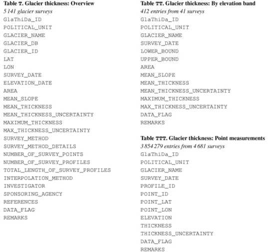
The data are structured as three relational database tables ordered in increasing level of detail (Fig. 2). The first, overview table (T) contains information on the location, identity, and area of the surveyed glacier; the survey method used; and details about the authors and sources of the data. Glacier mean and maximum thickness, estimated from point measurements, are also included when available from data providers. The second table (TT) contains any mean and maximum thicknesses, estimated from point measurements, for surface elevation bands. Although rare, some ice thick-ness surveys are only available as surface elevation band estimates, their point measurements having been lost or never published. The third table (TTT) contains point thick-ness measurements. All tables include a survey identifier (GlaThiDa_ID, unique in T) that links entries between the tables, as well as a country code (POLITICAL_UNIT) and glacier name (GLACIER_NAME), which are replicated in TT and TTT as a convenience to users. Structural changes since GlaThiDa v1, described in the changelog (Sect. 2.2.4), have been limited to adding fields (e.g., PROFILE_ID in v3 to group point measurements by survey profile) and renaming fields (e.g., DEM_DATE to ELEVATION_DATE in v3 to clar-ify that provided surface elevations need not be from a digital elevation model).
Following FAIR principles, the three tables are stored as CSV (comma-separated values) files, a universally supported
Table 1.Number of glacier surveys and point measurements, interquartile range of point thicknesses, and full range of survey years by survey method. In the database, a “survey” roughly represents one measurement campaign on one glacier, and a “point” represents a single ice thickness measurement (as opposed to a spatial mean).
Method Surveys Points Thickness (m) Years Radar (airborne) 4624 3 064 055 104–456 1968–2017 Radar (terrestrial) 412 700 066 87–330 1970–2018 Radar (both or unknown) 25 87 481 179–323 2006–2016 Seismic 43 31 218–440 1953–1993 Drilling 18 35 40–135 1935–2007 Electromagnetic 2 2611 47–86 2002–2002
Figure 1.Field photographs illustrating different methods for measuring glacier thickness. (a) Ground-penetrating radar measurements on Johnsons Glacier, Antarctica, in January 2020. The white sledge contains a radar transmitter, receiver, shielded antennas, control unit, and recording system. A Global Navigation Satellite System receiver antenna is mounted to the sledge. Credit: Francisco Navarro. (b) Aerial ground-penetrating radar measurements over Hansbreen, Svalbard, in spring 2011 (Navarro et al., 2014). The radar transmitter, receiver, and antennas are mounted to a wooden frame hung from the helicopter. Credit: Antoine Kies. (c) Hot water drilling on Rhonegletscher, Switzerland, in August 2018 by ETH Zurich’s Glacier Seismology Group. Although used mostly for characterizing bed conditions, the drillings measure ice thickness as a side product. Credit: Johannes Landmann. (d) Seismic reflection measurements on Grubengletscher, Switzerland, using a sledgehammer as a seismic energy source. The black seismic line connects geophones to the recording system. Credit: Bernd Kulessa.
text format for representing tabular data. To maximize ma-chine readability, the files do not contain any nondata content other than a single header line with field names. Data docu-mentation is performed by a separate metadata file, described below.
2.2.2 Metadata (datapackage.json)
The structure and content of the data package is described in a single JSON (JavaScript Object Notation) file which con-forms to the Frictionless Data Tabular Data Package specifi-cation (Walsh et al., 2017). This file contains general meta-data like the package’s name, version, description, and li-cense; a list of contributors; and links to published source datasets. The file also contains a detailed description of both the contents and structure of the tabular data files. In practice, CSV files come in a large number of variants; by making the format and character encoding explicit, we help both soft-ware and human users avoid unnecessary guesswork (Fig. 3). Each table field is described in turn, including its name and description, the data type it represents (string, integer, or floating point number), and any constraints on the values it can take (e.g., whether a value is required, falls within a numeric range, or matches a search pattern). In the example in Fig. 4, the description informs users that the field values are stored in the data files with “up to seven decimal places”, while the pattern \-?[0-9]*(\.[0-9]{1,7})? (a reg-ular expression conforming, as required by the Frictionless Data specification, to the XML Schema syntax; Biron and Malhotra, 2004) makes possible an automated test that this is indeed the case.
Finally, relations within and between tables are defined following relational database nomenclature. A unique key is a field (or set of fields) whose values must be unique for each row in the table. Unique keys can be stored in other ta-bles (where they are called “foreign keys”) to link the tata-bles together. In the example in Fig. 5, each row of table TTT (point measurements) is uniquely identified by the combina-tion of a survey identifier (GlaThiDa_ID), profile identifier (PROFILE_ID), and point identifier (POINT_ID). Each of these point measurements is linked to the corresponding row in table T (survey overviews) by the value of its survey identifier (GlaThiDa_ID), along with the replicated fields for country code (POLITICAL_UNIT) and glacier name (GLACIER_NAME).
2.2.3 Documentation (README.md)
The data package is fully described in datapackage.json, but the JSON format may not be familiar or welcoming to some users. Therefore, we automatically generate a more human-readable version from the contents of datapackage.json. The resulting README.md is a text file structured with Markdown, a widely supported markup language (Gruber, 2004). As a
result, it is both easy to read as plain text and readily con-verted to other formats such as HTML (Hypertext Markup Language) or PDF (Portable Document Format). The choice of file formats increases user access while their shared JSON origin eliminates the risks and overhead associated with manually maintaining multiple files.
2.2.4 History (CHANGELOG.md)
All notable changes made to the data or metadata are recorded in a chronological list formatted in Markdown, CHANGELOG.md. This includes the update or removal of existing data records, additions of new data records, and changes to the file structure or data schema. The goal is to provide a variety of user groups with important information about the history of the dataset. Future maintainers can re-view past changes, developers can evaluate whether and how to update their processing chain based on structural changes, and users can discover what data have been added or updated since the last version.
2.3 Product development cycle
The Glacier Thickness Database (GlaThiDa) is a community effort that grows as more data are collected. For an evolving dataset like ours, the ability to revise and review collabora-tively – to track changes and share those changes with oth-ers – is of great benefit to the communities that contribute to, maintain, and use the data. The development environment should therefore support the following activities:
– receive, review, and discuss issues with the dataset from and with the community;
– automatically track all changes made to the dataset by a distributed team of contributors;
– continuously validate the dataset as changes are made; – release new versions on a rolling basis, to be archived
– with a unique DOI (digital object identifier) for dis-tribution, citation, and safekeeping in a scientific data repository (Paskin, 2005).
2.3.1 Tooling
To achieve the goals listed above, we have adopted tools, widely used for open-source software development, for open-data development. In our case, the dataset is stored as a file repository managed by the distributed version con-trol system git and hosted on GitLab (https://gitlab.com, last access: 9 November 2020), an open-source equivalent of GitHub (https://github.com, last access: 9 November 2020), the popular online platform for collaborative software de-velopment. The underlying git software tracks changes (or “commits”), while GitLab provides interactive tools for gar-nering and managing input from the community. “Issues” –
Figure 2.Fields and overall contents of the three database tables T, TT, and TTT. Detailed field descriptions are provided in the metadata file described in Sect. 2.2.2.
Figure 3.Sample JSON from datapackage.json specifying the file format (format: “csv”), character encoding (encoding: “utf-8”), and structure of the data files – for example, that the first line of each file contains field names (header: true), values are separated by a comma (delimiter: “,”), and missing values are exclusively rep-resented by empty strings (missingValues: [“”]).
which can be posted by anyone with a free account – track bug reports, feature requests, and other community dialogue. “Releases” tag a snapshot of the dataset, at any stage in the development cycle, as a numbered version. These snapshots can then be assigned a DOI and placed in a scientific data repository for citing and safekeeping.
Version control systems like git are line based; that is, they track changes to text files on a line-by-line basis. Stor-ing all data and metadata as text files, rather than binary files, allows us to automatically track all changes to the dataset. When fixes are made to existing data records, the change con-sists of the updated lines. When new records are added, the change consists of the appended lines. In this way, we avoid making a new copy of a file each time a change is made. Only versions published for download by users are compressed to a binary format to reduce bandwidth.
2.3.2 Versioning
The project follows the Semantic Versioning Specification (Preston-Werner, 2013) for software, adapted for data. Given a version number major.minor.patch, the major ver-sion is incremented for new data, the minor verver-sion is
incre-Figure 4.Sample JSON from datapackage.json specifying the name, title, description, data type, and value constraints for the field POINT_LATin table TTT.
Figure 5.Sample JSON from datapackage.json specifying the unique keys and foreign keys for table TTT.
mented for changes to existing data, and the patch version is incremented for changes to metadata only.
Note that our versioning scheme does not communi-cate compatibility with downstream software dependencies, which is the primary purpose of semantic versioning. A proposed software-oriented alternative (Pollock and Walsh, 2017) is to increment the major version for incompati-ble changes (e.g., field removed, field constraint made more restrictive), the minor version for backwards-compatible changes (e.g., data added, field constraint made less restric-tive), and the patch version for backwards-compatible fixes (e.g., fix data errors, update field description). However, we believe our data-oriented versioning is better aligned with our users and contributors, who are primarily concerned with the addition of new data following each call for submissions.
2.3.3 Schema validation
A major benefit of describing the data with machine-readable metadata (i.e., datapackage.json) is the ability to au-tomatically validate the data against this description. This includes relations between tables, uniqueness within ta-bles, and whether field values match field types and con-straints: for example, whether dates match the expected for-mat (YYYYMMDD) and latitude and longitude are numbers within the allowed limits ([−90, 90] and [−180, 180]). Fur-thermore, by using a standard format for the metadata, we can automatically validate the metadata itself against this standard.
That said, all metadata standards have their limits; they cannot express all the possible constraints we may wish to impose on our data. In addition to tests of single fields, vali-dation of GlaThiDa includes tests across multiple fields – for
Figure 6. Sample Python code testing whether SURVEY_METHOD_DETAILS is provided whenever SURVEY_METHODis “OTH” (other).
example, that country codes (POLITICAL_UNIT) and point measurements (TTT.POINT_LAT, TTT.POINT_LON) are spatially consistent with the provided coordinates for the glacier center point (T.LAT, T.LON), or that survey method details (T.SURVEY_METHOD_DETAILS) are provided if the survey method (T.SURVEY_METHOD) is “other”. The latter test, implemented in Python, is shown in Fig. 6 as an example.
Continuous integration (CI) is a standard software devel-opment practice wherein changes to the code are verified by automated tests to detect and fix issues as quickly as pos-sible (Fowler, 2006). In our case, we use CI pipelines inte-grated into GitLab to automatically validate data and meta-data whenever a change is made to the repository, catching issues early in the development cycle and, crucially, before the next release.
3 Results and discussion 3.1 Spatial and temporal coverage
GlaThiDa v3 is the most comprehensive public database of glacier thickness measurements to date. We have added 3 million new thickness measurements relative to GlaThiDa v2, released in 2016 (Table 2). The new data, submitted by re-searchers or imported from the IceBridge data portal (https: //nsidc.org/data/icebridge, last access: 28 August 2019), in-clude glaciers in Antarctica, Alaska, Canada, China, Green-land, Kazakhstan, Norway, Svalbard, SwitzerGreen-land, and Tan-zania.
3.1.1 Spatial coverage
To evaluate the spatial coverage of GlaThiDa with respect to the world’s roughly 217 000 glaciers (RGI Consortium, 2017), we assigned each survey to glaciers in the Randolph Glacier Inventory (RGI 6.0) by intersecting point measure-ments and nominal glacier centerpoints with RGI glacier out-lines. The result is that 3054 RGI glaciers have thickness measurements in GlaThiDa (a large increase from 1133 RGI glaciers in version 2). Out of 5141 glacier surveys, only 11 (0.2 %) do not fall within an RGI glacier outline. Of these, most are for glaciers not included in RGI 6.0 – specifically, very small glaciers in the European Alps (Blauschnee and Glacier de Tsarmine, Switzerland; Schwarzmilzferner, Aus-tria) and glaciers that may be considered part of the Antarctic
Ice Sheet (Lambert Glacier, Starbuck Glacier, and Scharf-fenbergbotnen). The remaining do not intersect an RGI out-line because either the corresponding RGI outout-line is incor-rect (Nördlicher Schneeferner, Germany) or the glacier has retreated since the survey was conducted (Columbia Glacier, Alaska).
Figure 7 shows the coverage of intersected RGI glaciers on a world map. Table 3 lists the number and total area of inter-sected RGI glaciers by glacier region (GTN-G, 2017). While the proportion of intersected glaciers in a region is at most 14 % (region 7: Svalbard and Jan Mayen), the proportional area of intersected glaciers is much higher, up to 77 % (again, for Svalbard and Jan Mayen) – a result of larger glaciers be-ing preferentially selected for measurement. The coverage in Svalbard is so high in v3 thanks to a recent regional compila-tion of available measurements (Martín-Español et al., 2015; Fürst et al., 2018b). The regions with the next best area cover-age are those with substantial contributions from NASA Op-eration IceBridge: Arctic Canada, Antarctica, and Greenland. Despite these advances, large gaps persist in GlaThiDa, es-pecially throughout Asia, the Russian Arctic, and the Andes. Poor coverage in these regions necessarily limits the qual-ity of local and global glacier volume assessments and pre-dictions of future change. Future efforts should be aimed at increasing spatial coverage and regional representation, both by performing new measurements and by conducting litera-ture surveys and calls for data in underrepresented languages and regions of the world.
Overall, RGI glaciers with at least one thickness measure-ment account for 40 % (299 141 km2) of the global RGI area of 746 092 km2 (RGI Consortium, 2017). A better measure of data coverage is the area of a glacier that is within a cer-tain distance of a thickness point measurement located on the same glacier. Globally, 36 % of the area of all surveyed glaciers (102 030 km2), and 14 % of global glacier area, is within 1 km of a measurement. Although this represents a significant improvement over GlaThiDa v2 (6 %), this nev-ertheless means that the thickness of the vast majority of global glacier area must still be estimated through extrapo-lation, scaling methods (reviewed in Bahr et al., 2015), or models (reviewed in Farinotti et al., 2017).
The spatial coverage of point thickness measure-ments varies greatly by glacier. While 14 % of glaciers in GlaThiDa with point measurements have more than 100 point measurements km−2on average, 50 % have fewer than 18 points (Fig. 8). Although measurements are often sparse with respect to total glacier area, measurements tend to be well distributed across glacier surface elevations, since measurements are often collected along longitudinal pro-files. Dividing each glacier into 100 m elevation bands (cal-culated from the surface elevations of point measurements in GlaThiDa and the minimum and maximum glacier surface elevations in RGI), 50 % of glaciers with point measurements have measurements in at least half of their elevation bands and 11 % have measurements in all of their elevation bands.
Table 2. Total number of rows (surveys, elevation bands, or point measurements) and number of surveys represented in each table, by GlaThiDa version (“v”, with the release year in parentheses). Since not all glacier surveys have a mean glacier thickness in table T, such surveys are counted separately.
Table v1 (2014) v2 (2016) v3 (2019) T. Glacier thickness: Overview
Surveys (all) 1493 1601 5141 Surveys (with mean glacier thickness) 407 504 500 TT. Glacier thickness: By elevation band
Surveys represented 10 33 41 Elevation bands 175 376 412 TTT. Glacier thickness: Point measurements
Surveys represented 948 1080 4681 Point measurements 759 629 820 370 3 854 279
Table 3.GlaThiDa coverage for each glacier region mapped in Fig. 7. The count and total area (km2) of RGI glacier outlines with at least one (point, elevation band, or glacier-wide) thickness are listed for GlaThiDa v2 (2016) and v3 (2019) alongside the total for all RGI glaciers.
Region Name v2 (count) v3 (count) RGI (count) v2 (km2) v3 (km2) RGI (km2) 1 Alaska 14 41 27 108 4469 21 141 86 725 2 Western Canada and USA 38 45 18 855 118 142 14 524 3 Arctic Canada, North 239 476 4556 57 783 72 351 105 111 4 Arctic Canada, South 24 251 7415 10 633 13 943 40 888 5 Greenland periphery 295 1361 20 261 51 290 63 594 130 071 6 Iceland 4 4 568 2161 2161 11 060 7 Svalbard and Jan Mayen 79 232 1615 9582 26 318 33 959 8 Scandinavia 99 103 3417 800 813 2949 9 Russian Arctic 22 32 1069 3606 5716 51 592 10 Asia, North 20 61 5151 82 144 2410 11 Central Europe 128 175 3927 498 768 2092 12 Caucasus and Middle East 2 3 1888 5 36 1307 13 Asia, central 48 79 54 429 1466 1401 49 303 14 Asia, southwest 0 1 27 988 0 17 33 568 15 Asia, southeast 8 8 13 119 69 98 14 734 16 Low latitudes 6 9 2939 12 29 2341 17 Southern Andes 35 39 15 908 733 735 29 429 18 New Zealand 3 3 3 537 112 112 1162 19 Antarctic and subantarctic 69 131 2752 76 481 89 622 132 867 World 1133 3054 216 502 219 900 299 141 746 092
Glaciers with few measurements but well distributed along their length can still be very useful for validating modeled ice thicknesses (Castellani, 2019), which are often computed along longitudinal ice-flow lines (reviewed in Farinotti et al., 2017).
3.1.2 Temporal coverage
The glacier thickness surveys in GlaThiDa span the years 1935–2018 (Table 1). This wide range of survey dates en-ables glaciers with repeat surveys (such as the example in Fig. 9) to be compared over time. However, it also com-plicates regional and global studies, which must account
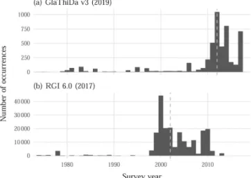
for thickness measurements spanning multiple years. Ideally, modeled ice thicknesses are evaluated against measured ice thicknesses coincident in time with the measured glacier out-lines, surface elevations, and other time-varying parameters (e.g., surface mass balance, rates of ice thickness change, and surface velocities) used to initialize the model (Farinotti et al., 2017). For analysis spanning many glaciers (or all of the world’s glaciers), it is not possible to ensure that all these data are coincident in time. For example, the median survey year for RGI glacier outlines is 2002, a decade earlier than the 2012 median for GlaThiDa surveys (Fig. 10), and the offset between surveys in GlaThiDa and their spatially coin-cident RGI outlines is 11–17 years (interquartile range). As
Figure 7.Map comparing GlaThiDa coverage to global glacier coverage according to the Randolph Glacier Inventory (RGI 6.0). Each grid cell represents 78.7 km × 78.7 km (roughly 1◦×1◦) in a cylindrical equal-area map projection. Light blue cells contain GlaThiDa data from IceBridge, while the overlaying dark blue pixels contain GlaThiDa data from other sources. Numbered grey polygons correspond to the glacier regions (GTN-G, 2017) listed in Table 3. Made with Natural Earth country polygons (https://www.naturalearthdata.com, last access: 23 October 2020).
for surface elevations, the majority (88 %) of point thickness measurements in GlaThiDa include corresponding surface elevations, 85 % of which were measured the same year as the ice thickness. When available, temporally coincident ice thickness and surface elevation measurements can be used to calculate the elevation of the glacier bed (independent of the survey date over decades to centuries) and thus the ice thickness relative to a glacier surface surveyed at any other time.
3.1.3 Future additions
Our intention is for GlaThiDa to continue to grow and improve as errors are found and fixed, new
measure-ments are made, and more data are found or submit-ted. Several datasets already published in open-data por-tals (e.g., https://data.npolar.no, last access: 25 March 2020; https://pangaea.de, last access: 25 March 2020; https:// arcticdata.io, last access: 25 March 2020; https://nsidc.org, last access: 25 March 2020, and https://www.usap-dc.org, last access: 25 March 2020) are slated for inclusion in a fu-ture version. However, these account for only a small num-ber of the glacier thickness measurements still missing in GlaThiDa. For example, 460 glacier surveys pulled from the literature for v1 (Gärtner-Roer et al., 2014) are still miss-ing the original point measurements from which the reported glacier-wide estimates were derived. An assessment of the Arctic data in GlaThiDa v2 by the Integrated Arctic
Obser-Figure 8. Number of RGI glaciers with point measurements in GlaThiDa by the average number of point measurements per square kilometer. The median (18 points km−2) is marked with a grey dashed line. Glaciers with a mean or maximum thickness but no point measurements are shown in the grey bar to the left of 0 km−2.
Figure 9. All thickness point measurements in GlaThiDa inter-secting the RGI outline (RGI60-07.01464) for Kronebreen, Sval-bard (78.992◦N, 13.384◦E), by survey date (or year, if the date is unknown). The corresponding studies referenced in GlaThiDa are Dowdeswell et al. (1984, 1986), Björnsson et al. (1996), Lindbäck et al. (2018), Kristensen et al. (2008), and Paden et al. (2018).
vation System (INTAROS, 2018) identified missing observa-tions and concluded that pressure must continue to be placed on research groups to submit their data to the wider commu-nity. Ideally, all ice thickness surveys would be published in open-data portals and then added to GlaThiDa for complete coverage in a standard format.
To streamline data aggregation going forward, GlaThiDa may need to be restructured such that data are primarily or-ganized by campaign or dataset rather than by glacier. The
Figure 10.Comparison of the distribution of survey years between GlaThiDa (a) and RGI (b). Medians are marked with grey dashed lines. Only survey years since 1975 are shown.
data tables were originally designed to accommodate mean glacier thicknesses pulled from the literature (Gärtner-Roer et al., 2014). Thus, each survey (i.e., each entry in table T, and thus each GlaThiDa_ID) is expected to contain mea-surements gathered on one visit to one glacier – even though each associated point (i.e., each entry in TTT) is also en-coded with temporal and spatial coordinates. This data model complicates the addition of large campaigns and introduces confusing redundancy to the database. For example, the six datasets from Operation IceBridge had to be split across 4124 glacier surveys by date and by intersection with RGI glacier outlines.
Operation IceBridge, the source of 61 % of the thick-ness point measurements in GlaThiDa, is ending operation in 2020. The airborne mission was designed to avoid a gap in measurements between the ICESat satellite (2003–2009) and its successor ICESat-2, which was launched in 2018. However, the ICESat satellites only measure surface eleva-tion and not ice thickness, therefore ending a decade-long ice thickness campaign. In the absence of a successor to Op-eration IceBridge, future updates to GlaThiDa may not in-clude as many new measurements as the latest version. How-ever, since RGI 6.0 does not include glaciers on the Antarc-tic Peninsula mainland (Huber et al., 2017) or in the Mc-Murdo Dry Valleys (Frank Paul, personal communication, 2020), IceBridge data for those glaciers were not included in GlaThiDa v3; these remaining IceBridge data will be added in a future version.
3.2 Thickness uncertainties
The uncertainty of a glacier thickness measurement varies widely with the method used, the characteristics of the site, and the interpretation of the raw data (reviewed in Gärtner-Roer et al., 2014, Sect. 3.2). For example, sources of error
for radar measurements (reviewed in Lapazaran et al., 2016a, Sect. 3.1) include the radio-wave velocity, the timing of the reflection, and migration (inverting for the reflection surface immediately below, rather than to the side), which can fail in or near steep terrain (Welch et al., 1998). Errors in the mea-surement position (e.g., due to the accuracy, placement, and movement of the GPS receiver) also translate to thickness er-rors proportional to the local thickness gradient (reviewed in Lapazaran et al., 2016a, Sect. 3.2). This is a larger issue for older data, especially those transformed from poorly defined coordinate systems or digitized from printed maps (e.g., An-dreassen et al., 2015).
The uncertainty of a spatially averaged thickness further varies with the adequacy of the interpolation (and extrapola-tion), the assumed glacier boundary and, most importantly, the spatial coverage of the measurements (reviewed in La-pazaran et al., 2016b). Thickness measurements are typi-cally acquired along sparse profiles, with coverage biased to-wards gentler terrain. Rarely, if ever, do they approximate a dense grid blanketing the whole glacier. From the law of er-ror propagation, we would expect measurement erer-rors to be smaller for spatial means. In practice, however, the opposite is more commonly the case, since measurement errors are of-ten partly spatially dependent (Martín-Español et al., 2016), rather than truly random, and point coverage is often far from ideal.
A fraction of glacier thicknesses in GlaThiDa were pub-lished with uncertainty estimates: 26 % of mean glacier thicknesses in table T (drawn from about 35 studies, based on the listed references), 19 % of mean elevation band thick-nesses in table TT (drawn from 4 studies), and 40 % of point thicknesses in table TTT (drawn from 51 studies). By com-puting percent uncertainties (100 %×uncertainty/thickness), we can compare the distribution of uncertainties by thick-ness type. We find that the reported uncertainties are signifi-cantly lower for point thicknesses than for the spatial means – an interquartile range of 3.1 %–5.5 % of the measured value for points versus 9.9 %–22.8 % and 20 %–50 % for glacier and elevation band means, respectively. The uncertainties re-ported by these studies may or may not be realistic. Never-theless, the relatively high uncertainties reported for spatial means clearly indicate that, for these studies, interpolation errors outweighed any benefit gained from averaging the spa-tially independent errors in the point measurements.
In practice, the statistical definition of the uncertainties re-ported in GlaThiDa is likely to vary considerably. For exam-ple, many studies do not specify whether or not a reported error is the standard deviation. Others may not necessarily provide a full error estimate but rather the “resolution of the measurements”, as in the case of some IceBridge datasets (MCoRDS, HiCARS, and PARIS). As pointed out by Martín-Español et al. (2016), based in part on two studies included in GlaThiDa (Pettersson et al., 2011; Saintenoy et al., 2013), er-rors for spatial means (e) in the literature can vary by orders of magnitude between two extreme assumptions:
(underes-timate) local errors (ei) are spatially independent, such that e = ¯ei/
√
n(where ¯ei is the mean of the local errors and n is their number), or (overestimate) local errors are linearly de-pendent, such that e = ¯ei (i.e., the mean of the local errors is taken as the error of the mean). As a consequence, we in-tend to tighten reporting requirements and flag statistically nonconforming uncertainties in future versions of GlaThiDa.
3.3 Data management 3.3.1 Error detection
As recorded in the changelog, we fixed a large number of er-rors introduced in previous versions and in the initial compi-lation of the current version. Many were trivial to fix once discovered; others required reviewing published literature and datasets, checking original submissions, and, if neces-sary, corresponding with the data provider. Most errors were detected by the suite of automated validation tests described in Sect. 2.3.3. Checks of field-level constraints identified missing values in required fields, duplicate values in unique fields, out-of-range values in numeric fields, invalid charac-ters in text fields, invalid values in enumerable fields, and future or nonexistent dates in date fields. Checks of table-level constraints identified duplicate values in unique keys (e.g., duplicate combinations of survey and point identifiers in TTT) and missing values in foreign keys (e.g., survey iden-tifiers in TT and TTT missing in T). More complex tests identified missing values that were required by logical im-plication (e.g., thickness missing when thickness uncertainty provided), values that were invalid by logical implication (e.g., glacier identifier not present in the glacier database to which it refers), and values that were invalid by spatial implication (e.g., glacier coordinates outside assigned coun-try or far from associated point measurements). Additional tests will necessarily need to be added proactively as the data evolve and retroactively as unforeseen errors are introduced and later discovered.
3.3.2 Data storage and version control
Every change, addition, and subtraction made to a file in the data package is tracked by git. As the number of changes grows over time, the git repository will inevitably grow in size. Cloud-storage hosts place storage limits on free ac-counts: GitLab.com limits repositories to 10 GB compressed; GitHub.com limits repositories to 100 GB and each file to 100 MB uncompressed. To keep repositories small in the presence of large files, git-lfs (Git Large File Storage) was developed to track files in the repository while storing them externally (Carlson and Schneider, 2019). However, whether the file is binary or text, a new copy of the file is made for each change – no matter how small the change. By storing our data as text files in the repository, changes are stored incrementally, which imparts significant storage bene-fits. At the time of writing, the repository is only 47.9 MB
compressed despite 121 changes, including 8 versions of TTT.csv (294 MB uncompressed, 42.3 MB compressed). Reaching the 10 GB storage limit on GitLab.com would re-quire adding (or changing) roughly 1 billion point measure-ments. If this limit were ever reached, it could be lifted by migrating to a self-hosted GitLab installation.
Nevertheless, line-based version control systems like git are not optimized for tracking changes to tabular data. A change to a single cell is recorded as a change to the entire row, and swapping the order of two columns is recorded as a change of every row in the table (Fitzpatrick, 2013). Changes to tabular data can be described more compactly (and leg-ibly) using specialized syntax (e.g., Tabular Diff Specifica-tion; Fitzpatrick, 2014), but these impart no storage benefit unless the underlying version control systems were rewrit-ten to use them to store changes internally. Alternatively, many changes can be described as operations rather than as changes to file content, such as a log of Structured Query Language (SQL) commands to a relational database or the change history tracked by OpenRefine (Hirst, 2013). How-ever, these would require specific software and a strict (and nonstandard) workflow to make changes to the data.
4 Data availability
GlaThiDa is maintained as a git repository hosted at https://gitlab.com/wgms/glathida (last access: 9 Novem-ber 2020). Bug reports, data submissions, and other is-sues should be posted to the issue tracker at https:// gitlab.com/wgms/glathida/-/issues (last access: 9 Novem-ber 2020). Published versions of GlaThiDa – those with an assigned DOI (digital object identifier) – are hosted by the World Glacier Monitoring Service (WGMS) in Zurich, Switzerland (e.g., v3.1.0, from which this paper was generated: https://doi.org/10.5904/wgms-glathida-2020-10, GlaThiDa Consortium, 2020). GlaThiDa is licensed un-der Creative Commons Attribution 4.0 International (CC-BY-4.0: https://creativecommons.org/licenses/by/4.0, last ac-cess: 9 November 2020).
5 Conclusions
The Glacier Thickness Database (GlaThiDa) has been es-tablished as the international data repository for glacier ice thickness observations. Version 3 contains standardized data for roughly 3000 glaciers worldwide, collected from in situ and airborne measurements. Overall, 14 % of global glacier area is now within 1 km of a thickness measurement (located on the same glacier), although large regional gaps persist, es-pecially in Asia, the Russian Arctic, and the Andes. Thanks to simple metadata formats and a development environment based on open-source software, GlaThiDa fulfills the FAIR principles (Findable, Accessible, Interoperable and Reusable for both machines and people) and surpasses them with
auto-matic version control, continuous validation, and an interface for community dialogue. Hosted by the World Glacier Moni-toring Service (WGMS), GlaThiDa will continue to serve the glaciological community as a trustworthy dataset.
Team list. The additional contributors listed below helped com-pile earlier versions of GlaThiDa, performed measurements, pro-cessed data, and/or submitted data to GlaThiDa. They are listed be-low in alphabetical order by last name. This list does not include the authors of published literature and datasets which were added to GlaThiDa by the authors of GlaThiDa. Affiliations were recorded at the time of contribution and may not be current.
Jakob Abermann (Asiaq Greenland Survey, Greenland), Song-tao Ai (Wuhan University, China), Brian Anderson (Victoria Uni-versity of Wellington: Antarctic Research Centre, New Zealand), Serguei M. Arkhipov (Russian Academy of Sciences: Institute of Geography, Russia), Izumi Asaji (Hokkaido University, Japan), An-dreas Bauder (Swiss Federal Institute of Technology (ETH) Zürich: Laboratory of Hydraulics, Hydrology and Glaciology (VAW), Switzerland), Jostein Bakke (University of Bergen: Department of Earth Sciences, Norway), Toby J. Benham (Scott Polar Research In-stitute, United Kingdom), Douglas I. Benn (University of Saint An-drews, United Kingdom), Daniel Binder (Central Institute for Me-teorology and Geodynamics (ZAMG), Austria), Elisa Bjerre (Tech-nical University of Denmark: Arctic Technology Centre, Denmark), Helgi Björnsson (University of Iceland, Iceland), Norbert Blindow (Institute for Geophysics, University of Münster, Germany), Pas-cal Bohleber (Austrian Academy of Sciences (ÖAW): Institute for Interdisciplinary Mountain Research (IGF), Austria), Eliane Brän-dle (University of Fribourg, Switzerland), Gino Casassa (University of Magallanes: GAIA Antarctic Research Center (CIGA), Chile), Jorge Luis Ceballos (Institute of Hydrology, Meteorology and En-vironmental Studies (IDEAM), Colombia), Julian A. Dowdeswell (Scott Polar Research Institute, United Kingdom), Felipe An-dres Echeverry Acosta (Hallgeir Elvehøy – Norwegian Water Re-sources and Energy Directorate (NVE), Norway), Rune Engeset (Norwegian Water Resources and Energy Directorate (NVE), Nor-way), Andrea Fischer (Institute of Interdisciplinary Mountain Re-search (IGF), Austria), Mauro Fischer (University of Fribourg, Switzerland), Gwenn E. Flowers (Simon Fraser University: De-partment of Earth Sciences, Canada), Erlend Førre (University of Bergen: Department of Earth Sciences, Norway), Yoshiyuki Fu-jii (National Institute of Polar Research, Japan), Mariusz Gra-biec (University of Silesia in Katowice, Poland), Jon Ove Ha-gen (University of Oslo, Norway), Svein-Erik Hamran (University of Oslo, Norway), Lea Hartl (Institute of Interdisciplinary Moun-tain Research (IGF), Austria), Robert Hawley (Dartmouth Col-lege, United States), Kay Helfricht (Institute of Interdisciplinary Mountain Research (IGF), Austria), Elisabeth Isaksson (Norwe-gian Polar Institute, Norway), Jacek Jania (University of Sile-sia in Katowice, Poland), Robert W. Jacobel (Saint Olaf Col-lege: Physics Department, United States), Michael Kennett (Nor-wegian Water Resources and Energy Directorate (NVE), Norway), Bjarne Kjøllmoen (Norwegian Water Resources and Energy Di-rectorate (NVE), Norway), Thomas Knecht (University of Zürich, Switzerland), Jack Kohler (Norwegian Polar Institute, Norway), Vladimir Kotlyakov (Russian Academy of Sciences: Institute of Ge-ography, Russia), Steen Savstrup Kristensen (Technical University
of Denmark: Department of Space Research and Space Technology (DTU Space), Denmark), Stanislav Kutuzov (University of Read-ing, United Kingdom), Javier Lapazaran (Universidad Politécnica de Madrid, Spain), Tron Laumann (Norwegian Water Resources and Energy Directorate (NVE), Norway), Ivan Lavrentiev (Rus-sian Academy of Sciences: Institute of Geography, Russia), Ka-trin Lindbäck (Norwegian Polar Institute, Norway), Peter Lisager (Asiaq Greenland Survey, Greenland), Francisco Machío (Univer-sidad Internacional de La Rioja (UNIR), Spain), Gerhard Markl (Institute of Interdisciplinary Mountain Research (IGF), Austria), Enrico Mattea (University of Fribourg: Department of Geography, Switzerland), Kjetil Melvold (Norwegian Water Resources and En-ergy Directorate (NVE), Norway), Laurent Mingo (Blue System Integration Ltd., Canada), Christian Mitterer (Institute of Interdis-ciplinary Mountain Research (IGF), Austria), Andri Moll (Uni-versity of Zürich, Switzerland), Ian Owens (Uni(Uni-versity of Can-terbury: Department of Geography, New Zealand), Finnur Páls-son (University of Iceland, Iceland), Rickard PettersPáls-son (Uppsala University, Sweden), Rainer Prinz (University of Graz: Depart-ment of Geography and Regional Science, Austria), Jaan-Mati Pun-ning (Estonian Academy of Sciences (USSR Academy of Sciences-Estonia): Institute of Geology, Estonia), Antoine Rabatel (Univer-sity Grenoble Alpes, France), Ian Raphael (Dartmouth College, United States), David Rippin (University of York, United King-dom), Andrés Rivera (Center for Scientific Studies (CECs), Chile), José Luis Rodríguez Lagos (Center for Scientific Studies (CECs), Chile), John Sanders (University of California, Berkeley: Depart-ment of Earth and Planetary Science, United States), Albane Sain-tenoy (University of Paris-Sud, France), Arne C. Sætrang (Nor-wegian Polar Institute, Norway), Marius Schaefer (Austral Uni-versity of Chile: Institute of Physical and Mathematical Sciences (ICFM), Chile), Stefan Scheiblauer (Environmental Earth Obser-vation Information Technology (ENVEO IT GmbH), Austria), Thomas V. Schuler (University of Oslo, Norway), Heïdi Sevestre (University of Saint Andrews, United Kingdom), Bernd Seiser (stitute of Interdisciplinary Mountain Research (IGF), Austria), In-gvild Sørdal (University of Oslo: Department of Geosciences, Nor-way), Jakob Steiner (University of Utrecht: Faculty of Geosciences, the Netherlands), Peter Alexander Stentoft (Technical University of Denmark: Arctic Technology Centre (ARTEK), Denmark), Mar-tin Stocker-Waldhuber (Technical University of Denmark: Arc-tic Technology Centre (ARTEK), Denmark), Bernd Seiser (In-stitute of Interdisciplinary Mountain Research (IGF), Austria), Shin Sugiyama (Hokkaido University: Institute of Low Tempera-ture Science, Japan), Rein Vaikmäe (Tallinn University of Technol-ogy, Estonia), Evgeny Vasilenko (Academy of Sciences of Uzbek-istan, Uzbekistan), Nat J. Wilson (Simon Fraser University: Depart-ment of Earth Sciences, Canada), Victor S. Zagorodnov (Russian Academy of Sciences: Institute of Geography, Russia), and Ro-drigo Zamora (Center for Scientific Studies (CECs), Chile).
Author contributions. MZ conceived the project. EW designed and implemented the data package and development environment, with input from MZ. EW prepared the manuscript, with feedback from MZ, FN, MH, JJF, IGR, JL, HM, KN, LMA, DF, and HL. MZ, FN, MH, JJF, IGR, JL, HM, and KN helped compile earlier versions of GlaThiDa. LMA, DF, and HL cochaired the International Asso-ciation of Cryospheric Sciences (IACS) Working Group on Glacier
Ice Thickness Estimation. Additional contributors are named in the Team list.
Competing interests. The authors declare that they have no con-flict of interest.
Acknowledgements. This work is a contribution to the Interna-tional Association of Cryospheric Sciences (IACS) Working Group on Glacier Ice Thickness Estimation (https://cryosphericsciences. org/activities/ice-thickness, last access: 9 November 2020). We are grateful to NASA Operation IceBridge and the National Snow and Ice Data Center for making their data publicly available online. We thank the countless people who contributed to the planning, exe-cution, and processing of glacier thickness measurements included in GlaThiDa who are not named in the Team list. Institutions that funded the acquisition, processing, and archiving of thickness mea-surements included in GlaThiDa are acknowledged in the database.
Financial support. This research has been supported by the In-ternational Association of Cryospheric Sciences and by the Fed-eral Office of Meteorology and Climatology (MeteoSwiss) within the framework of the Global Climate Observing System (GCOS) in Switzerland.
Review statement. This paper was edited by Prasad Gogineni and reviewed by Bruce Raup, Aparna Shukla, and one anonymous referee.
References
Anderton, P. W.: Tasman Glacier 1971–73, no. 33, in: Hydrological Research Annual Report, Ministry of Works and Development for the National Water and Soil Conservation Organisation, New Zealand, 1975.
Andreassen, L., Huss, M., Melvold, K., Elvehøy, H., and Winsvold, S.: Ice Thickness Measurements and Volume Es-timates for Glaciers in Norway, J. Glaciol., 61, 763–775, https://doi.org/10.3189/2015JoG14J161, 2015.
Aric, K. and Brückl, E.: Eisdickenmessungen auf Gletschern der Ostalpen, in: Die Zentralanstalt für Meteorologie und Geody-namik 1851-2001: 150 Jahre Meteorologie und Geophysik in Österreich, edited by: Hammerl, C., Lenhardt, W., Steinacker, R., and Steinhauser, P., pp. 768–780, Leykam, Graz, Austria, available at: https://geschichte.univie.ac.at/en/node/14118 (last access: 9 November 2020), 2001.
Ayala, Á., Farías-Barahona, D., Huss, M., Pellicciotti, F., McPhee, J., and Farinotti, D.: Glacier runoff variations since 1955 in the Maipo River basin, in the semiarid Andes of central Chile, The Cryosphere, 14, 2005–2027, https://doi.org/10.5194/tc-14-2005-2020, 2020.
Bahr, D. B., Pfeffer, W. T., and Kaser, G.: A Review of Volume-Area Scaling of Glaciers, Rev. Geophys., 53, 95–140, https://doi.org/10.1002/2014RG000470, 2015.
Biron, P. V. and Malhotra, A.: XML Schema Part 2: Datatypes Second Edition. Appendix F: Regular Expressions, W3C Rec-ommendation, World Wide Web Consortium, available at: https: //www.w3.org/TR/xmlschema-2/#regexs (last access: 9 Novem-ber 2020), 2004.
Björnsson, H., Gjessing, Y., Hamran, S.-E., Hagen, J. O., Liestøl, O., Pálsson, F., and Erlingsson, B.: The Ther-mal Regime of Sub-Polar Glaciers Mapped by Multi-Frequency Radio-Echo Sounding, J. Glaciol., 42, 23–32, https://doi.org/10.3189/S0022143000030495, 1996.
Blankenship, D. D., Kempf, S. D., Young, D. A., Richter, T. G., Schroeder, D. M., Greenbaum, J. S., Holt, J. W., van Ommen, T., Warner, R. C., Roberts, J. L., Young, N. W., Lemeur, E., and Siegert, M. J.: IceBridge HiCARS 1 L2 Geolocated Ice Thick-ness, Version 1, https://doi.org/10.5067/F5FGUT9F5089, 2017a. Blankenship, D. D., Kempf, S. D., Young, D. A., Richter, T. G., Schroeder, D. M., Ng, G., Greenbaum, J. S., van Ommen, T., Warner, R. C., Roberts, J. L., Young, N. W., Lemeur, E., and Siegert, M. J.: IceBridge HiCARS 2 L2 Geolocated Ice Thick-ness, Version 1, https://doi.org/10.5067/9EBR2T0VXUDG, 2017b.
Blischak, J. D., Davenport, E. R., and Wilson, G.: A Quick Introduc-tion to Version Control with Git and GitHub, PLOS Computa-tional Biology, 12, https://doi.org/10.1371/journal.pcbi.1004668, 2016.
Carlson, B. M. and Schneider, L. X.: Git-Lfs, Git LFS, available at: https://github.com/git-lfs/git-lfs (last access: 9 November 2020), 2019.
Castellani, M.: An Overview of the Glacier Thickness Database, available at: https://oggm.org/2019/03/21/GlaThiDa-statistics (last access: 9 November 2020), 2019.
Cerri, D. and Fuggetta, A.: Open Standards, Open For-mats, and Open Source, J. Syst. Software, 80, 1930–1937, https://doi.org/10.1016/j.jss.2007.01.048, 2007.
Chacon, S. and Straub, B.: Pro Git, Apress, New York, NY, USA, second edn., available at: https://git-scm.com/book/en/v2 (last access: 9 November 2020), 2014.
Dowdeswell, J. A., Drewry, D. J., Liestøl, O., and Orheim, O.: Airborne Radio Echo Sounding of Sub-Polar Glaciers in Spitsbergen, no. 182 in Skrifter, Norsk Polarinstitutt, Oslo, Norway, available at: https://brage.npolar.no/npolar-xmlui/ bitstream/handle/11250/173505/Skrifter182.pdf (last access: 9 November 2020), 1984.
Dowdeswell, J. A., Drewry, D. J., Cooper, A. P. R., Gorman, M. R., Liestøl, O., and Orheim, O.: Digital Mapping of the Nordaust-landet Ice Caps from Airborne Geophysical Investigations, Ann. Glaciol., 8, 51–58, https://doi.org/10.3189/S0260305500001130, 1986.
Farinotti, D., Brinkerhoff, D. J., Clarke, G. K. C., Fürst, J. J., Frey, H., Gantayat, P., Gillet-Chaulet, F., Girard, C., Huss, M., Leclercq, P. W., Linsbauer, A., Machguth, H., Martin, C., Maus-sion, F., Morlighem, M., Mosbeux, C., Pandit, A., Portmann, A., Rabatel, A., Ramsankaran, R., Reerink, T. J., Sanchez, O., Stentoft, P. A., Singh Kumari, S., van Pelt, W. J. J., An-derson, B., Benham, T., Binder, D., Dowdeswell, J. A., Fis-cher, A., Helfricht, K., Kutuzov, S., Lavrentiev, I., McNabb, R., Gudmundsson, G. H., Li, H., and Andreassen, L. M.: How accurate are estimates of glacier ice thickness? Results from ITMIX, the Ice Thickness Models Intercomparison
eXperi-ment, The Cryosphere, 11, 949–970, https://doi.org/10.5194/tc-11-949-2017, 2017.
Farinotti, D., Huss, M., Fürst, J. J., Landmann, J., Machguth, H., Maussion, F., and Pandit, A.: A Consensus Estimate for the Ice Thickness Distribution of All Glaciers on Earth, Nat. Geosci., 12, 168–173, https://doi.org/10.1038/s41561-019-0300-3, 2019. Finn, C. A., Deszcz-Pan, M., and Bedrosian, P. A.: Helicopter
Electromagnetic Data Map Ice Thickness at Mount Adams and Mount Baker, Washington, USA, J. Glaciol., 58, 1133–1143, https://doi.org/10.3189/2012JoG11J098, 2012.
Fischer, A., Mitterer, C., Stocker-Waldhuber, M., Binder, D., and Dinale, R.: Ice Thickness Measurements on South Tyrolean Glaciers 1996–2014, Pangaea, https://doi.org/10.1594/PANGAEA.849390, 2015a.
Fischer, A., Span, N., Kuhn, M., Helfricht, K., Stocker-Waldhuber, M., Seiser, B., Massimo, M., and Butschek, M.: Ground-Penetrating Radar (GPR) Point Measurements of Ice Thickness in Austria, Pangaea, https://doi.org/10.1594/PANGAEA.849497, 2015b.
Fischer, M.: Understanding the Response of Very Small Glaciers in the Swiss Alps to Climate Change, PhD, University of Fribourg, Fribourg, Switzerland, available at: https://www.researchgate. net/publication/323839822_Understanding_the_response_of_ very_small_glaciers_in_the_Swiss_Alps_to_climate_change (last access: 9 November 2020), 2018.
Fitzpatrick, P.: Diffing and Patching Tabular Data, available at: http: //okfnlabs.org/blog/2013/08/08/diffing-and-patching-data.html (last access: 9 November 2020), 2013.
Fitzpatrick, P.: Tabular Diff Specification, Version 0.8, avail-able at: http://paulfitz.github.io/daff-doc/spec.html (last access: 9 November 2020), 2014.
Fowler, D., Barratt, J., and Walsh, P.: Frictionless Data: Making Research Data Quality Visible, International Journal of Digital Curation, 12, 274–285, https://doi.org/10.2218/ijdc.v12i2.577, 2017.
Fowler, M.: Continuous Integration, available at: https: //martinfowler.com/articles/continuousIntegration.html (last access: 9 November 2020), 2006.
Fürst, J. J., Navarro, F., Gillet-Chaulet, F., Huss, M., Moholdt, G., Fettweis, X., Lang, C., Seehaus, T., Ai, S., Benham, T. J., Benn, D. I., Björnsson, H., Dowdeswell, J. A., Grabiec, M., Kohler, J., Lavrentiev, I., Lindbäck, K., Melvold, K., Pettersson, R., Rippin, D., Saintenoy, A., Sánchez-Gámez, P., Schuler, T. V., Sevestre, H., Vasilenko, E., and Braun, M. H.: The Ice-Free To-pography of Svalbard, Geophys. Res. Lett., 45, 11760–11769, https://doi.org/10.1029/2018GL079734, 2018a.
Fürst, J. J., Navarro, F., Gillet-Chaulet, F., Huss, M., Moholdt, G., Fettweis, X., Lang, C., Seehaus, T., Ai, S., Benham, T. J., Benn, D. I., Björnsson, H., Dowdeswell, J. A., Gra-biec, M., Kohler, J., Lavrentiev, I., Lindbäck, K., Melvold, K., Pettersson, R., Rippin, D., Saintenoy, A., Sánchez-Gámez, P., Schuler, T. V., Sevestre, H., Vasilenko, E., and Braun, M. H.: SVIFT1.0 - The Svalbard Ice-Free Topography [v1.0], https://doi.org/10.21334/npolar.2018.57fd0db4, 2018b. Gärtner-Roer, I., Naegeli, K., Huss, M., Knecht, T., Machguth,
H., and Zemp, M.: A Database of Worldwide Glacier Thick-ness Observations, Global Planet. Change, 122, 330–344, https://doi.org/10.1016/j.gloplacha.2014.09.003, 2014.
GlaThiDa Consortium: Glacier Thickness Database 3.1.0, https://doi.org/10.5904/wgms-glathida-2020-10, 2020.
GLIMS and NSIDC: GLIMS Glacier Database, https://doi.org/10.7265/N5V98602, 2018.
Gruber, J.: Markdown 1.0.1, available at: https://daringfireball.net/ projects/markdown/ (last access: 9 November 2020), 2004. GTN-G: GTN-G Glacier Regions,
https://doi.org/10.5904/gtng-glacreg-2017-07, 2017.
Hirst, T.: Diff or Chop? Github, CSV Data Files and Open-Refine, available at: https://blog.ouseful.info/2013/08/27/ diff-or-chop-github-csv-data-files-and-openrefine/ (last access: 9 November 2020), 2013.
Huber, J., Cook, A. J., Paul, F., and Zemp, M.: A complete glacier inventory of the Antarctic Peninsula based on Landsat 7 images from 2000 to 2002 and other preexisting data sets, Earth Syst. Sci. Data, 9, 115–131, https://doi.org/10.5194/essd-9-115-2017, 2017.
INTAROS: Report on Present Observing Capacities and Gaps: Land and Cryosphere | Integrated Arctic Observation System, Research and Innovation Action under European Commission Horizon2020 Deliverable 2.7, Integrated Arctic Observation System (INTAROS), Nansen Environmental and Remote Sens-ing Center, Norway, available at: https://intaros.nersc.no/content/ report-present-observing-capacities-and-gaps-land-and-cryosphere (last access: 9 November 2020), 2018.
Jania, J., Mochnacki, D., and Gadek, B.: The Thermal Structure of Hansbreen, a Tidewater Glacier in Southern Spitsbergen, Svalbard, Polar Res., 15, 53–66, https://doi.org/10.1111/j.1751-8369.1996.tb00458.x, 1996.
Koenig, L., Martin, S., Studinger, M., and Sonntag, J.: Po-lar Airborne Observations Fill Gap in Satellite Data, Eos, Transactions American Geophysical Union, 91, 333–334, https://doi.org/10.1029/2010EO380002, 2010.
Kotlyakov, V. M., Arkhipov, S. M., Henderson, K. A., and Nagornov, O. V.: Deep Drilling of Glaciers in Eurasian Arc-tic as a Source of PaleoclimaArc-tic Records, Quaternary Sci. Rev., 23, 1371–1390, https://doi.org/10.1016/j.quascirev.2003.12.013, 2004.
Kristensen, S. S., Christensen, E. L., Hanson, S., Reeh, N., Sk-ourup, H., and Stenseng, L.: Airborne Ice-Sounder Survey of the Austfonna Ice Cap and Kongsfjorden Glacier at Svalbard, May 3rd, 2007, Field report, DTU Space, Copenhagen, Den-mark, available at: https://orbit.dtu.dk/en/publications/airborne-ice-sounder-survey-of-the-austfonna-ice-cap-and-kongsfjo (last access: 9 November 2020), 2008.
Lapazaran, J. J., Otero, J., Martín-Español, A., and Navarro, F. J.: On the Errors Involved in Ice-Thickness Estimates I: Ground-Penetrating Radar Measurement Errors, J. Glaciol., 62, 1008– 1020, 2016a.
Lapazaran, J. J., Otero, J., Martín-Español, A., and Navarro, F. J.: On the Errors Involved in Ice-Thickness Estimates II: Errors in Digital Elevation Models of Ice Thickness, J. Glaciol., 62, 1021– 1029, https://doi.org/10.1017/jog.2016.94, 2016b.
Lindbäck, K., Kohler, J., Pettersson, R., Nuth, C., Langley, K., Messerli, A., Vallot, D., Matsuoka, K., and Brandt, O.: Sub-glacial topography, ice thickness, and bathymetry of Kongsfjor-den, northwestern Svalbard, Earth Syst. Sci. Data, 10, 1769– 1781, https://doi.org/10.5194/essd-10-1769-2018, 2018.
Martín-Español, A., Vasilenko, E. V., Navarro, F. J., Otero, J., La-pazaran, J. J., Lavrentiev, I., Macheret, Y. Y., and Machío, F.: Radio-Echo Sounding and Ice Volume Estimates of Western Nor-denskiöld Land Glaciers, Svalbard, Ann. Glaciol., 54, 211–217, https://doi.org/10.3189/2013AoG64A109, 2013.
Martín-Español, A., Navarro, F. J., Otero, J., Lapazaran, J. J., and Błaszczyk, M.: Estimate of the Total Volume of Svalbard Glaciers, and Their Potential Contribution to Sea-Level Rise, Us-ing New Regionally Based ScalUs-ing Relationships, J. Glaciol., 61, 29–41, https://doi.org/10.3189/2015JoG14J159, 2015.
Martín-Español, A., Lapazaran, J. J., Otero, J., and Navarro, F. J.: On the Errors Involved in Ice-Thickness Esti-mates III: Error in Volume, J. Glaciol., 62, 1030–1036, https://doi.org/10.1017/jog.2016.95, 2016.
Meyer, C. R., Downey, A. S., and Rempel, A. W.: Freeze-on Limits Bed Strength beneath Sliding Glaciers, Nat. Commun., 9, 1–6, https://doi.org/10.1038/s41467-018-05716-1, 2018.
Navarro, F. J., Martín-Español, A., Lapazaran, J. J., Grabiec, M., Otero, J., Vasilenko, E. V., and Puczko, D.: Ice Volume Esti-mates from Ground-Penetrating Radar Surveys, Wedel Jarlsberg Land Glaciers, Svalbard, Arctic Antarct. Alp. Res., 46, 394–406, https://doi.org/10.1657/1938-4246-46.2.394, 2014.
Paden, J., Li, J., Leuschen, C., Rodriguez-Morales, F., and Hale, R.: Pre-IceBridge MCoRDS L2 Ice Thickness, Version 1, https://doi.org/10.5067/QKMTQ02C2U56, 2011.
Paden, J., Li, J., Leuschen, C., Rodriguez-Morales, F., and Hale, R.: IceBridge MCoRDS L2 Ice Thickness, Version 1, https://doi.org/10.5067/GDQ0CUCVTE2Q, 2018.
Paskin, N.: Digital Object Identifiers for Scientific Data, Data Sci. J., 4, 12–20, https://doi.org/10.2481/dsj.4.12, 2005.
Pettersson, R., Christoffersen, P., Dowdeswell, J. A., Pohjola, V. A., Hubbard, A., and Strozzi, T.: Ice Thickness and Basal Conditions of Vestfonna Ice Cap, Eastern Svalbard, Geograf. Anna. Ser. A, 93, 311–322, https://doi.org/10.1111/j.1468-0459.2011.00438.x, 2011.
Pollock, R. and Walsh, P.: Patterns: Data Package Ver-sion, available at: https://specs.frictionlessdata.io//patterns/ #data-package-version (last access: 9 November 2020), 2017. Preston-Werner, T.: Semantic Versioning 2.0.0, available at: https:
//semver.org/spec/v2.0.0.html (last access: 9 November 2020), 2013.
Ram, K.: Git Can Facilitate Greater Reproducibility and In-creased Transparency in Science, Source Code for Biology and Medicine, 8, 7, https://doi.org/10.1186/1751-0473-8-7, 2013. Raney, K.: IceBridge PARIS L2 Ice Thickness, Version 1,
https://doi.org/10.5067/OMEAKG6GIJNB, 2010.
Rauber, A., Asmi, A., van Uytvanck, D., and Proell, S.: Data tion of Evolving Data, Tech. rep., Working Group on Data Cita-tion (WGDC), https://doi.org/10.15497/RDA00016, 2015. RGI Consortium: Randolph Glacier Inventory (RGI 3.2),
https://doi.org/10.7265/N5-RGI-32, 2013.
RGI Consortium: Randolph Glacier Inventory (RGI 6.0), https://doi.org/10.7265/N5-RGI-60, 2017.
Rignot, E., Mouginot, J., Larsen, C. F., Gim, Y., and Kirch-ner, D.: Low-Frequency Radar Sounding of Temperate Ice Masses in Southern Alaska, Geophys. Res. Lett., 40, 5399–5405, https://doi.org/10.1002/2013GL057452, 2013a.
Rignot, E., Mouginot, J., Larsen, C. F., Gim, Y., and Kirchner, D.: IceBridge WISE L2 Ice Thickness and Surface Elevation, Ver-sion 1, https://doi.org/10.5067/0ZBRL3GY720R, 2013b. Rutishauser, A., Maurer, H., and Bauder, A.:
Helicopter-Borne Ground-Penetrating Radar Investigations on Temper-ate Alpine Glaciers: A Comparison of Different Systems and Their Abilities for Bedrock mappingHelicopter GPR on Temperate Glaciers, Geophysics, 81, WA119–WA129, https://doi.org/10.1190/geo2015-0144.1, 2016.
Saintenoy, A., Friedt, J.-M., Booth, A. D., Tolle, F., Bernard, E., Laffly, D., Marlin, C., and Griselin, M.: Deriving Ice Thick-ness, Glacier Volume and Bedrock Morphology of Austre Lovén-breen (Svalbard) Using GPR, Near Surf. Geophys., 11, 253–262, https://doi.org/10.3997/1873-0604.2012040, 2013.
Schroeder, D. M., Bingham, R. G., Blankenship, D. D., Chris-tianson, K., Eisen, O., Flowers, G. E., Karlsson, N. B., Koutnik, M. R., Paden, J. D., and Siegert, M. J.: Five Decades of Radioglaciology, Annals of Glaciology, pp. 1–13, https://doi.org/10.1017/aog.2020.11, 2020.
Shi, L., Allen, C. T., Ledford, J. R., Rodriguez-Morales, F., Blake, W. A., Panzer, B. G., Prokopiack, S. C., Leuschen, C. J., and Gogineni, S.: Multichannel Coherent Radar Depth Sounder for NASA Operation Ice Bridge, in: 2010 IEEE International Geoscience and Remote Sensing Symposium, pp. 1729–1732, https://doi.org/10.1109/IGARSS.2010.5649518, 2010.
Susstrunk, A.: Sondage du glacier par la méthode sismique [Sound-ing of the glacier by the seismic method], La Houille Blanche, pp. 309–318, https://doi.org/10.1051/lhb/1951010, 1951. Thorlaksson, D.: Calibrating a Glacier Ice Thickness Inversion
Model from In-Situ Point Measurements, M.S., University of Innsbruck, Innsbruck, Austria, available at: http://diglib.uibk. ac.at/ulbtirolhs/download/pdf/1945420 (last access: 9 Novem-ber 2020), 2017.
Walsh, P., Pollock, R., and Keegan, M.: Tabular Data Pack-age, Version 1, available at: https://specs.frictionlessdata.io/ /tabular-data-package (last access: 9 November 2020), 2017. Welch, B. C., Pfeffer, W. T., Harper, J. T., and Humphrey,
N. F.: Mapping Subglacial Surfaces of Temperate Valley Glaciers by Two-Pass Migration of a Radio-Echo Sounding Survey, J. Glaciol., 44, 164–170, https://doi.org/10.3189/S0022143000002458, 1998.
Werder, M. A., Huss, M., Paul, F., Dehecq, A., and Farinotti, D.: A Bayesian Ice Thickness Estimation Model for Large-Scale Applications, J. Glaciol., 66, 137–152, https://doi.org/10.1017/jog.2019.93, 2020.
WGMS: Glacier Thickness Database 1.0, https://doi.org/10.5904/wgms-glathida-2014-09, 2014.
WGMS: Glacier Thickness Database 2.1, https://doi.org/10.5904/wgms-glathida-2016-07, 2016.
WGMS and NSIDC: World Glacier Inventory, https://doi.org/10.7265/N5/NSIDC-WGI-2012-02, 2012. Wilkinson, M. D., Dumontier, M., Aalbersberg, I. J., Appleton, G.,
Axton, M., Baak, A., Blomberg, N., Boiten, J.-W., da Silva San-tos, L. B., Bourne, P. E., Bouwman, J., Brookes, A. J., Clark, T., Crosas, M., Dillo, I., Dumon, O., Edmunds, S., Evelo, C. T., Finkers, R., Gonzalez-Beltran, A., Gray, A. J. G., Groth, P., Goble, C., Grethe, J. S., Heringa, J., ’t Hoen, P. A. C., Hooft, R., Kuhn, T., Kok, R., Kok, J., Lusher, S. J., Martone, M. E., Mons, A., Packer, A. L., Persson, B., Rocca-Serra, P., Roos, M., van Schaik, R., Sansone, S.-A., Schultes, E., Sengstag, T., Slater, T., Strawn, G., Swertz, M. A., Thompson, M., van der Lei, J., van Mulligen, E., Velterop, J., Waagmeester, A., Wittenburg, P., Wol-stencroft, K., Zhao, J., and Mons, B.: The FAIR Guiding Princi-ples for Scientific Data Management and Stewardship, Sci. Data, 3, 1–9, https://doi.org/10.1038/sdata.2016.18, 2016.