HAL Id: hal-03100758
https://hal.inrae.fr/hal-03100758
Submitted on 4 May 2021
HAL is a multi-disciplinary open access archive for the deposit and dissemination of sci-entific research documents, whether they are pub-lished or not. The documents may come from teaching and research institutions in France or abroad, or from public or private research centers.
L’archive ouverte pluridisciplinaire HAL, est destinée au dépôt et à la diffusion de documents scientifiques de niveau recherche, publiés ou non, émanant des établissements d’enseignement et de recherche français ou étrangers, des laboratoires publics ou privés.
discrimination of untargeted metabolomic urine analysis:
results from a comparative study
Loïc Mervant, Marie Tremblay-Franco, Emilien L. Jamin, Emmanuelle
Kesse-Guyot, Pilar Galan, Jean-Francois Martin, Françoise Guéraud, Laurent
Debrauwer
To cite this version:
Loïc Mervant, Marie Tremblay-Franco, Emilien L. Jamin, Emmanuelle Kesse-Guyot, Pilar Galan, et al.. Osmolality-based normalization enhances statistical discrimination of untargeted metabolomic urine analysis: results from a comparative study. Metabolomics, Springer Verlag, 2021, 17 (1), �10.1007/s11306-020-01758-z�. �hal-03100758�
https://doi.org/10.1007/s11306-020-01758-z ORIGINAL ARTICLE
Osmolality‑based normalization enhances statistical discrimination
of untargeted metabolomic urine analysis: results from a comparative
study
Loïc Mervant1,2 · Marie Tremblay‑Franco1,2 · Emilien L. Jamin1,2 · Emmanuelle Kesse‑Guyot3 · Pilar Galan3 · Jean‑François Martin1,2 · Françoise Guéraud2 · Laurent Debrauwer1,2
Received: 18 June 2020 / Accepted: 9 December 2020 / Published online: 2 January 2021
© The Author(s), under exclusive licence to Springer Science+Business Media, LLC part of Springer Nature 2021
Abstract
Introduction Because of its ease of collection, urine is one of the most commonly used matrices for metabolomics studies.
However, unlike other biofluids, urine exhibits tremendous variability that can introduce confounding inconsistency during result interpretation. Despite many existing techniques to normalize urine samples, there is still no consensus on either which method is most appropriate or how to evaluate these methods.
Objectives To investigate the impact of several methods and combinations of methods conventionally used in urine
metabo-lomics on the statistical discrimination of two groups in a simple metabometabo-lomics study.
Methods We applied 14 different strategies of normalization to forty urine samples analysed by liquid chromatography coupled to high-resolution mass spectrometry (LC-HRMS). To evaluate the impact of these different strategies, we relied on the ability of each method to reduce confounding variability while retaining variability of interest, as well as the predict-ability of statistical models.
Results Among all tested normalization methods, osmolality-based normalization gave the best results. Moreover, we demon-strated that normalization using a specific dilution prior to the analysis outperformed post-acquisition normalization. We also demonstrated that the combination of various normalization methods does not necessarily improve statistical discrimination.
Conclusions This study re-emphasized the importance of normalizing urine samples for metabolomics studies. In addition, it appeared that the choice of method had a significant impact on result quality. Consequently, we suggest osmolality-based normalization as the best method for normalizing urine samples.
Trial registration number: NCT03335644
Keywords Untargeted metabolomics · Urine analysis · Normalization · Mass spectrometry · Osmolality
1 Introduction
Along with other omics approaches, such as transcriptom-ics and proteomtranscriptom-ics, metabolomtranscriptom-ics methods are now widely used to probe qualitative and quantitative variations in endogenous metabolites to assess the impact of various diseases or environmental conditions on metabolic homeo-stasis (Jansson et al. 2009; Wikoff et al. 2009). The study of metabolome modulation constitutes a powerful approach since the metabolome represents the most direct link to the phenotype compared to other “omics” (Fiehn 2002). Nuclear magnetic resonance (NMR) and mass spectrometry (MS) are now established as the reference techniques used in metabolomics. NMR is known to be more robust than MS but also to give access to a smaller set of metabolites due to
Supplementary informtaion The online version of this article (https ://doi.org/10.1007/s1130 6-020-01758 -z) contains supplementary material, which is available to authorized users. * Marie Tremblay-Franco
marie.tremblay-franco@inrae.fr
1 Metatoul-AXIOM Platform, MetaboHUB, Toxalim, INRAE,
Toulouse, France
2 Toxalim, Toulouse University, INRAE, ENVT, INP-Purpan,
UPS, Toulouse, France
3 Sorbonne Paris Nord University, Inserm, INRAE, Cnam,
Nutritional Epidemiology, Research Team (EREN), Epidemiology and Statistics Research Center – University of Paris (CRESS), 93017 Bobigny, France
a lower sensitivity. Considering this lower sensitivity, MS is generally more widely used than NMR for metabolomics studies and will be the focus of this article. Among the vari-ous matrices analysed in metabolomics, urine is one of the most commonly used because of the non-invasive nature of its collection and the quantity of available samples. How-ever, in contrast to other biofluids, such as plasma and cer-ebrospinal fluid, urine is far less regulated and can exhibit up to 14-fold variation in total metabolite concentrations (Warrack et al. 2009). Focusing on urine, numerous nor-malization strategies have emerged to mitigate the varia-tions that are mainly attributable to non-relevant parameters such as hydration level, which can bias conclusions based on changes in metabolite concentration and introduces con-founding factors.
Several normalization techniques based on various fac-tors have been proposed for normalizing metabolomics data. Among them, as proposed by Edmands et al. (2014) and more recently by Gagnebin et al. (2017), two different approaches can be distinguished, namely, pre-analysis nor-malization often based on a biological parameter such as creatinine, specific gravity, and osmolality (Chen et al. 2013; Vogl et al. 2016; Warrack et al. 2009), and post-acquisition curative normalization. The creatinine concentration is one of the most commonly used reference factors because the urinary creatinine level is supposed to reflect the overall concentration of metabolites (Ryan et al. 2011). Indeed, creatinine excretion levels are assumed to remain constant within and across individuals since they are linked to muscle degradation and glomerular filtration (Waikar et al. 2010). However, its use as a normalization factor is currently under debate since factors such as diet, muscle mass, age, physi-cal activity and menstrual cycle can affect creatinine levels (Cross et al. 2011; Davison and Noble 1981; Décombaz et al.
1979; James et al. 1988; Skinner et al. 1996). The urine volume excreted during 24 h is also used as a normalization factor for metabolomics studies (Godzien et al. 2011) (Shih et al. 2019), but this parameter is not always accessible, especially in the case of human samples. Osmolality, which is considered one of the most reliable methods for evaluating overall urine metabolite concentration (Chadha et al. 2001), can also be used as a normalization factor in metabolomics (Yamamoto et al. 2019). The advantage of measuring osmo-lality is that it is only influenced by the number of particles and chemical entities dissolved in urine, thus better reflect-ing the overall urine metabolite concentration than creatinine level or total urine volume. However, osmolality measure-ment requires specific equipmeasure-ment. Directly linked to osmo-lality and more easily routinely measurable, specific grav-ity is also used to estimate urine metabolite concentrations in metabolomics studies (Edmands et al. 2014). However, this parameter, representing the ratio between the mass of a given volume of urine and the mass of the same volume
of water, less faithfully reflects the solute concentration, is more prone to measurement errors due to the presence of large molecules (Chadha et al. 2001; Cook et al. 2020; Voinescu et al. 2002) and requires larger sample volumes. Other data, such as the total NMR signal, can also be used to estimate the overall urine metabolite concentration. It should be noted that all these parameters can be used pre-analysis by applying specific dilutions or post acquisition by dividing the signal of detected metabolites. As reviewed by Wu and Li (2016), sample normalization methods in metabolomics are diverse and vary from one study to another, as well as the conclusion of studies evaluating the performance of nor-malization methods. In their study, Vogl et al. concluded that creatinine was the most efficient normalization method, even over osmolality (Vogl et al. 2016), while more recently, Rosen Vollmar et al. and Burton et al. determined that spe-cific gravity was more reliable than creatinine (Burton et al.
2014; Rosen Vollmar et al. 2019), and others found better results with osmolality normalization (Chetwynd et al. 2016; Gagnebin et al. 2017).
In line with the diversity of pre-analytical normalization techniques, the post-analytical panel of approaches is also very diverse. Some of the most employed post-acquisition normalization methods, such as total ion current (TIC) normalization, MS total useful signal (MSTUS) (Warrack et al. 2009) or probabilistic quotient normalization (PQN) (Dieterle et al. 2006), are based on a ratio between each feature and a given spectral reference. With TIC normali-zation, each feature intensity is divided by the sum of all feature intensities in the sample of interest. As TIC nor-malization is sensitive to orphan features and xenobiot-ics, Warrack et al. (2009) proposed MSTUS normalization based on a normalization factor calculated from features common to all samples. This technique assumes that the number of decreasing and increasing metabolites is rela-tively equivalent across the samples, although this condi-tion is not always met in all studies (Jacob et al. 2014). Initially, proposed to normalize NMR metabolomics data, the PQN method was also used to normalize MS metabo-lomics data. This method is based on the calculation of a dilution coefficient in relation to a reference spectrum, such as the median of quality control (QC) samples. In addition to these normalization methods, which aim to correct concentration differences, other algorithms such as LOESS (Dunn et al. 2011) have been used to correct analytical drift, which is of particular importance in MS-based metabolomics. In the face of this diversity, some tools, such as NormalizeMets (De Livera et al. 2018) or Normalyzer (Chawade et al. 2014), have been developed to evaluate the performance of various normalization meth-ods for metabolomics data. Despite these tools, there is at present no consensus on the use of normalization methods in metabolomics or on how to evaluate their performances.
Here, we propose to evaluate the performance of several of the most employed metabolomics data normalization methods on the basis of a simple metabolomics study carried out by liquid chromatography mass spectrometry (LC–MS) on urine samples. As the conclusions of the literature remain unclear, it is still necessary to conduct multiple studies eval-uating normalization methods to draw general conclusions. A cohort of forty individuals free of pathological conditions (that could bias normalization based on biological factors such as creatinine or osmolality) was chosen to perform this study. Considering this particular design relying on subjects from the general population, we suggest that extrapolation of our study results could be more generally applicable than those obtained from studies comparing a control popula-tion to a diseased populapopula-tion that may bias normalizapopula-tion. The impact of specific dilutions of samples to normalize either creatinine or osmolality was studied and compared with post-acquisition normalization using these parameters, as well as the PQN and MSTUS mathematical normaliza-tion methods. A total of 14 normalizanormaliza-tion strategies were tested and compared. The comparison was based on several complementary criteria, including intra-group variance and residual variability reduction, percentage of explained bio-logical variability of interest, and finally predictive capacity of statistical models.
2 Materials and methods
2.1 Chemicals
All solvents were purchased from Fisher Scientific (Thermo Fisher Scientific, Illkirch, France) and were of LC–MS grade.
2.2 Sample preparation
Urine samples were collected from forty healthy indi-viduals (20 women and 20 men) from the NutriNet-Santé study, an ongoing web-based observational prospective study launched in France in 2009 (Hercberg et al. 2010) and including adult volunteers. The NutriNet-Santé study was conducted according to the Declaration of Helsinki guidelines and was approved by the Institutional Review Board of the French Institute for Health and Medical Research (IRB Inserm n°0000388FWA00005831) and the “Commission Nationale de l’Informatique et des Libertés” (CNILn°908450/n°909216). Clinicaltrials.govnumber: NCT03335644. At the clinical visit, urine sample collec-tion was performed using vessels allowing for closed-circuit urine transfer from the vessel to a Vacutainer® tube. Urine samples were collected either in autumn/winter (n = 23) or spring/summer (n = 17) from 2011 to 2014. The Vacutainer®
tubes containing the spot urine samples were kept at + 4 °C before and during transportation to the central laboratory. After splitting into aliquots, urine samples were stored at − 80 °C for further analyses. Samples were divided into three parts and were prepared as follows: the first part of the samples was diluted 1:3 (v/v) in LC mobile phase A (95:5 water/methanol + 0.1% acetic acid). The second part of the samples was diluted to standardize creatinine concentration based on the smallest value, determined by 1H NMR accord-ing to a method adapted from Bouatra et al. (Bouatra et al.
2013), and then diluted 1:3 (v/v) in mobile phase A. The third part was specifically diluted to standardize osmolality levels based on the smallest value, determined using a freez-ing point osmometer (Loeser Messtechnik, Berlin, Germany) and then diluted 1:3 (v/v) in mobile phase A. After dilution, all samples were vortexed and centrifuged at 9500×g for 5 min. The supernatant was collected and transferred into vials to be directly analysed by UHPLC-MS. QC samples were prepared by pooling equivalent volumes of all samples. QCs were diluted to obtain dQC samples.
2.3 Instrumentation
LC–MS analyses were performed using an ultra-per-formance liquid chromatography (UPLC) instrument (ACQUITY, Waters, Manchester, UK) coupled to a quad-rupole time-of-flight mass spectrometer (Q-ToF Synapt G2-Si, Waters, Manchester, UK) as previously described (Jamin et al. 2020). A volume of 10 µL was injected into a Hypersil Gold C18 (1.9 μm, 100 mm × 2.1 mm) analyti-cal column (Thermo Fisher Scientific, Illkirch, France) at a flow rate of 0.3 mL/min and maintained at 40 °C. A linear gradient programme was set up with mobile phase A: 95% H2O/5% methanol/0.1% acetic acid, and mobile phase B:
100% methanol/0.1% acetic acid. The initial conditions were 100% A, followed by a linear gradient from 0 to 100% B in 30 min. These conditions were held for 4 min prior to switching in 1 min to the starting conditions that were held for 5 min to equilibrate the column. Samples were analysed in three analytical batches, and QC samples were injected at the beginning of each batch and then every six samples to evaluate analytical drift.
Full MS acquisitions were achieved with electrospray ionization in negative mode as follows: capillary voltage, 0.5 kV; sampling cone voltage, 30 V; source temperature, 120 °C; desolvation temperature, 550 °C; cone gas (N2) flow
rate, 30 L/h; and desolvation gas (N2) flow rate, 600 L/h.
Data were acquired from mass-to-charge ratios (m/z) of 50 to 800. Internal mass calibration was performed by injecting leucine enkephalin at 1 ng/mL at a flow rate of 10 µL/min. Data were acquired by operating the Synapt spectrometer in sensitivity mode and using dynamic range extension (DRE) to enhance both the sensitivity and dynamic range.
2.4 Data processing
Metabolomics data are complex, and there are multiple sources of variability, so it is sometimes difficult to iso-late variability due to biological factors of interest. For this reason, it is necessary to define and identify the dif-ferent sources of variability to apply appropriate filters and decrease some unwanted variabilities. It is therefore mandatory to distinguish between variability linked to the biological factor studied, which is called biological vari-ability of interest, and varivari-ability not linked to the biologi-cal factor. The latter can be divided into several factors, such as technical variability, confounding biological vari-ability and residual varivari-ability. Technical varivari-ability can, for instance, originate from sample preparation or analyti-cal drift. Confounding biologianalyti-cal variability is related to a known biological factor other than the factor of interest (e.g., biofluid concentration, BMI, etc.). Finally, residual variabil-ity corresponds to the remaining variabilvariabil-ity not explained by these previous factors. Full-HRMS data were processed using XCMS 3.0 with the collaborative environment Work-flow4Metabolomics (W4M) dedicated to the processing of metabolomics data (Giacomoni et al. 2015). Extraction of data from full scan spectra was carried out using the cent-wave algorithm (ppm = 10, peak width = (5,40), sntresh = 10, noise = 10,000, bw = 10, mzwid = 0.01). Data were then fil-tered using a ratio of the average signal in QCs over the average signal in blanks with a threshold of 3. We also elimi-nated all features displaying a correlation coefficient with dQC samples lower than 0.6. LOESS regression was applied based on QC samples to correct intra- and inter-batch drift. At the end, only common features displaying an RSD lower than 30% in QC samples were retained. PQN and MSTUS
normalization were performed using the W4M environment. For PQN normalization, the median of the QCs was chosen as a reference.
2.5 Tested normalization strategies
The combination of pre- and post-acquisition normaliza-tions led to the test of fourteen strategies of normalization presented in Table 1.
2.6 Statistical analyses
Statistical analyses were performed using Simca-P 14.0 software (Umetrics, Umea, Sweden) and MATLAB 2017b (The MathWorks, Inc.). All data were log transformed and Pareto scaled prior to principal component analysis (PCA) and orthogonal partial least square discriminant analysis (OPLS-DA). Log transformation was applied to reduce heteroscedasticity (Li et al. 2016) and Pareto to reduce the differences in intensity between features without increasing the analytical noise too much (Yang et al. 2015). PCA mod-els were assessed using the explained variance parameter (R2), and the number of principal components was chosen
based on a scree plot (Cattell 1966). Predictive capacity (Q2) and permutation tests were used to check the validity
and robustness of the O-PLS-DA models. Q2, whose
val-ues are between 0 and 1, corresponds to the fraction of the total variation of the biological factor of interest that can be predicted by the O-PLS-DA model. The permutation test assesses whether the specific classification of individuals in the two designated groups is significantly better than any other random classification in two arbitrary groups (West-erhuis et al. 2008). A model is considered robust when it
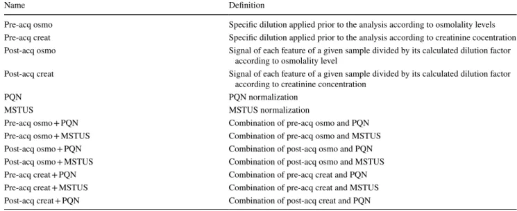
Table 1 Description of the fourteen normalization techniques assessed in this work
Name Definition
Pre-acq osmo Specific dilution applied prior to the analysis according to osmolality levels Pre-acq creat Specific dilution applied prior to the analysis according to creatinine cocentration Post-acq osmo Signal of each feature of a given sample divided by its calculated dilution factor
according to osmolality level
Post-acq creat Signal of each feature of a given sample divided by its calculated dilution factor according to creatinine concentration
PQN PQN normalization
MSTUS MSTUS normalization
Pre-acq osmo + PQN Combination of pre-acq osmo and PQN Pre-acq osmo + MSTUS Combination of pre-acq osmo and MSTUS Post-acq osmo + PQN Combination of post-acq osmo and PQN Post-acq osmo + MSTUS Combination of post-acq osmo and MSTUS Pre-acq creat + PQN Combination of pre-acq creat and PQN Pre-acq creat + MSTUS Combination of pre-acq creat and MSTUS Post-acq creat + PQN Combination of post-acq creat and PQN
displays a Q2 intercept < 0.05 (Lapins et al. 2008). When the optimal number of orthogonal components was higher than 1, the orthogonal component was manually added as long as the percentage of explained variance by this component was higher than 5%. The numbers of predictive and orthogonal components included in the OPLSDA models are displayed in Supplementary Material S2. Seven-fold cross-validation was used to estimate the predictive ability of the adjusted model (Q2). However, O-PLS-DA cannot separate
variabil-ity corresponding to the different factors of the experimen-tal design (sex and normalization in this study). To reach this, analysis of variance multiblock orthogonal partial least squares (AMOPLS) (Boccard and Rudaz 2016) was applied to assess the percentage of explained variance associated with each factor of the experimental design. This method works in two steps. In the first step, total variability is split according to the factors (normalization, sex and interaction, in this study). The significance of each effect is tested based on the permutation test (Vis et al. 2007). Then, multiblock OPLS was used to fit a multivariate model based on subma-trices obtained from ANOVA decomposition.
3 Results and discussion
The objective of this work was to evaluate the performance of several of the most employed normalization methods for urine metabolomics. Urine samples from forty male and female individuals were analysed by UPLC-MS with or without normalization by specific dilution prior to acquisi-tion. Data obtained from samples without pre-acquisition dilution were used to evaluate the impact of pre- and post-acquisition normalization. The evaluation of the perfor-mance of these different strategies was carried out based on the predictive ability of the generated statistical models, as well as the percentage of variance that could be attributed to the biological factor of interest, i.e., sex, in this study. Since metabolomics aims to highlight quantitative or qualitative differences in metabolite levels as a function of a biologi-cal factor, an ideal normalization method would reduce the variability not linked to the factor of interest while retaining the maximum amount of information related to the studied condition.
3.1 Urine exhibits a large concentration distribution
Creatinine concentrations and osmolality were measured to estimate the overall sample concentration, allowing for the calculation of individual dilution factors to normalize either creatinine concentrations or osmolality levels. A large distribution of concentration levels was observed, ranging from 1.67 to 20.27 mol/L for creatinine and from 217 to
1236 mOsmol for osmolality (Supplementary S1). Sur-prisingly, a significant difference was observed (Wilcoxon paired test, significance threshold 0.05) between calculated dilution factors from creatinine and osmolality, as shown in Fig. 1a. Dilution factors ranged from 1 to 12 for creatinine and from 1 to 5.7 for osmolality. Despite this disparity, a good correlation (r = 0.87) was observed between the dilu-tion factors calculated from the two parameters, as presented in Fig. 1b, indicating that both of these estimators are suita-ble to evaluate the overall metabolite concentration in urine. Because creatinine normalized samples are more diluted, the number of values missing before the FillPeaks step in the XCMS process was studied. No major differences were found between the three conditions, even a slight decrease in the number of missing values was observed with creatinine-normalized samples (data not shown).
Fig. 1 Concentration variations in urine samples. a Dilution factors calculated for both creatinine and osmolality. b Correlation of dilu-tion factors calculated according to creatinine levels and osmolality levels
To ensure that urine normalization based on these two parameters would not introduce bias in the discrimination of the two population groups, univariate statistical analyses (Mann–Whitney test, significance threshold 0.05) were per-formed on creatinine and osmolality levels, and no signifi-cant differences between men and women were observed for either of these parameters (data not shown). These results underlined the large concentration distribution in urine sam-ple metabolite concentrations.
3.2 Normalization decreases overall variability
As shown in Sect. 3.1 osmolality levels and creatinine concentrations exhibit large variations that were possibly responsible for a large part of the sample set variability. Dilution according to creatinine and osmolality levels aimed to normalize the dataset and reduce the variability linked to overall urinary concentration.
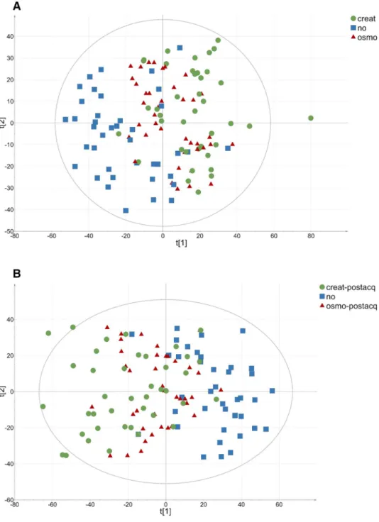
To assess the impact of normalization methods on the overall variability, which corresponds to both biological variability and variability not linked to the factor of inter-est, PCA was first performed on log-transformed data. This allowed for the comparison of the non-normalized dataset to the pre- and post-acquisition normalized datasets using both creatinine and osmolality-based normalization. A total of 4758 out of the 17,366 initially detected features were kept after the filtration process and subjected to PCA. The variance in the coordinates of individuals in each dataset on the first two components was calculated to assess the impact of normalization on data dispersion. As displayed in Fig. 2a, samples diluted according to osmolality levels (red triangles) exhibit less dispersion on the PCA plot than sam-ples adjusted according to creatinine concentration (green circles) or non-normalized samples (blue squares). This observation was confirmed by calculating the variance of individuals in each dataset where osmolality normalization showed a strong decrease in overall variance (var = 257.9) compared to creatinine normalization (var = 375.2) or the non-normalized dataset (var = 422.32).
Post-acquisition normalization achieved by dividing the signal intensity of each feature for a given sample by the cal-culated dilution factor was also assessed. The latter approach is less constrained since post-acquisition normalization avoids pre-acquisition sample dilution by a pre-determined factor, which can be tedious, especially with large sample cohorts. For the pre-acquisition normalized samples, PCA was performed from the non-normalized dataset and the dataset normalized by dilution factors calculated either from creatinine or osmolality levels. As presented in Fig. 2b, when compared to the non-normalized dataset (var = 524.5), vari-ances in the coordinates of individuals showed a decrease in overall variability when normalization was performed on
osmolality (var = 329.4) levels but not with creatinine-based normalization (var = 582.6).
These results suggest that regardless of the strategy employed, osmolality-based normalization leads to a lower overall variability than the other normalization methods. PCA combining all datasets was performed to determine which of the pre-acquisition or post-acquisition strategies led to the greatest reduction in overall variability. The vari-ance in coordinates was 239.2 for diluted samples and 329.4 for post-acquisition normalized samples (data not shown), suggesting that post-acquisition normalization is less effi-cient than pre-acquisition normalization for decreasing global variability. This can be tentatively explained by the fact that major differences in urine concentration induce strong differences in matrix effects, which can lead to ion suppression in MS analyses and thus to an increase in signal variability. Therefore, using a specific dilution to standard-ize urine concentration prior to mass spectrometric analysis could decrease the differences in matrix effects linked to urine concentration.
3.3 Normalization improves statistical discrimination
Most metabolomics studies are based on the comparison of relative metabolite abundances between two or more groups. As a consequence, decreasing variability not linked to the biological factor by applying normalization techniques would result in an increase in the statistical discrimination of groups. In this study, to assess the effect of various nor-malization methods, we relied on the statistical power of supervised OPLS-DA models to discriminate two groups composed of 20 men or 20 women.
Fourteen normalization strategies were tested and com-pared with the non-normalized dataset chosen as the refer-ence. The results displayed in Fig. 3 show that statistical models built with the pre-acquisition normalized dataset led to better results than those built with the non-normalized dataset (grey line), especially for osmolality normalization in terms of the predictive ability of the model (Q2 = 0.52).
Q2 values for all models are displayed in Supplementary S2
These results are in accordance with the decrease in overall variability observed in Fig. 2, suggesting that pre-acquisition normalization reduced variability not linked to the biological factor of interest while retaining biological information, according to Fig. 3. On the other hand, pre-acquisition normalization according to creatinine concen-tration only led to a slight improvement in statistical segre-gation (Q2 = 0.42) compared to the non-normalized dataset
(Q2 = 0.35). Interestingly, when normalization was
per-formed on osmolality or creatinine levels after data acqui-sition, no improvement was observed for fitted OPLS-DA
models, although a reduction in overall variability was observed, especially for osmolality normalization.
We further tested whether post-acquisition methods such as PQN (Dieterle et al. 2006) or MSTUS (Warrack et al. 2009) could supplant pre-acquisition normalization for improving statistical discrimination. We observed that PQN led to similar results (Q2 = 0.33) as MSTUS
(Q2 = 0.33), explained by the fact that we kept only
fea-tures that were common to all samples during the data filtration. Indeed, the first step of the PQN normalization consisted of a TIC normalization before performing a nor-malization with respect to a reference sample (i.e., the
median of QCs samples in this case). As all the features of the dataset were shared between all the samples, MSTUS normalization corresponded here to TIC normalization. Thus, in this particular case, the only difference between PQN and MSTUS normalization was the division by a constant determined by the median of the QC samples and thus led to the same results. By comparing the results obtained with mathematical post-acquisition methods to those obtained with pre-acquisition normalization, post-acquisition methods were found to be less efficient than specific dilutions. Finally, the combination of both biological- and mathematical-based normalization was
Fig. 2 Two-dimensional PCA score plot of HR-MS spectra of urine samples. Each symbol represents an individual data point projected onto the first (horizontal axis) and second (vertical axis) PCA compo-nents. Normalization methods are shown in different colours: creatinine in green dots (n = 40), none in blue squares (n = 40), and osmolality in red triangles (n = 40). The black ellipse determines the 95% confidence interval, which was drawn using Hotelling’s T2 statistic. a Preac-quisition normalization: A = 2, R2 = 20%. b Post-acquisition normalization: A = 2, R2 = 24% (Colour figure online)
investigated. No statistical improvement was observed when applying this combination (Q2 = 0.33).
Surpris-ingly, when combining two post-acquisition methods, the results were identical. Indeed, this combination consists of dividing a feature by its calculated dilution factor and then by the sum of features itself divided by the same dilution constant. In total, this nullifies the post-acquisi-tion normalizapost-acquisi-tion based on the dilupost-acquisi-tion factor. However, when pre- and post-acquisition methods were combined, no statistical improvement was observed, suggesting that part of the biological variability associated with sex was removed by this sequential process. Indeed, the statistical model performed with the Pre-acq osmo dataset led to bet-ter predictivity (Q2 = 0.52) than the models resulting from
the combination of Pre-acq osmo with MSTUS (Q2 = 0.46)
or with PQN (Q2 = 0.46). The same results were obtained
for the creatinine normalized dataset.
Taken together, these results showed that the applied nor-malization method can act on the predictability of a statisti-cal model. In total, 6 out of the 14 tested normalizations led to an increase in the discrimination power of the adjusted models, and notable differences were observed between normalization strategies. Normalization by specific dilution according to osmolality levels outperformed other meth-ods. Interestingly, no improvement (and even a decrease in predictability) was obtained when applying this method in combination with PQN or MSTUS.
3.4 Pre‑acquisition normalization reduces residual variability
To further investigate the link between the overall decrease in variability and the statistical power improvement, the ability of these various normalization strategies to reduce residual variability while keeping biological information was investigated by splitting the total variance into parts corresponding to the different factors based on AMOPLS.
As presented in Fig. 4a, the percentage of variability asso-ciated with sex ranged from 2.9 to 3.6% depending on the applied normalization method. In line with previous find-ings, normalization by specific dilution based on osmolality levels corresponded to the higher percentage of variabil-ity explained by sex with 3.6% variability. Post-acquisition normalization based on osmolality or creatinine levels did not lead to such an improvement, although the percentage of variability explained by sex was higher than that in the refer-ence dataset. Interestingly, no differrefer-ence was observed when applying post-acquisition methods such as PQN or MSTUS compared to the non-normalized dataset. This is also in accordance with our previous results and suggests that over-normalization can reduce variability with a negative impact on the discrimination power. Despite the slight improvement in the percentage of variability linked to sex, it is noteworthy that sex was only a significant factor (p = 0.04, 500 permu-tations) when pre-acquisition osmolality normalization is
Fig. 3 Radar chart of Q2 of
OPLS-DA models generated for all tested normalization strate-gies (blue line) compared to Q2
of OPLS-DA generated from non-normalized model (grey line). For detailed values of Q2,
see Supplementary S2 (Colour figure online)
performed, in contrast to other tested normalizations. Resid-ual variability, which corresponds to unexplained variance, can mask variability linked to sex. An ideal method would reduce residual variability while increasing the percentage of variance explained by the biological factor of interest. As illustrated in Fig. 4b, residual variability was also affected by normalization. The lowest residual variability was associated with the pre-acquisition normalization based on osmolality levels with 75% residual variability, while it was between 75 and 76.5% for other normalizations. Here, again, the
combination of methods with MSTUS or PQN or the use of PQN or MSTUS alone did not lead to a greater reduction in residual variability.
These findings are in accordance with previous obser-vations, showing that the statistical improvement observed in Sect. 3.3 for pre-acquisition osmolality-based dilution is linked to a decrease in residual variability and an increase in the percentage of variance associated with the biological effect.
4 Conclusion
Normalization of data is often a pre-requisite for obtain-ing unbiased results in statistical analyses. When applied to metabolomics data, normalization is especially important for matrices such as urine, which are highly variable. Four-teen normalization strategies often used in metabolomics were compared to determine the most suitable normaliza-tion for urine metabolomics, considering their performance for overall variability reduction, enhancement of statisti-cal power and unwanted variability reduction. Our results showed that the normalization method using urine-specific dilution according to osmolality levels gave the best results. Surprisingly, the combination of this method with PQN or MSTUS did not improve our assessment criteria and even led to a decrease in statistical discrimination, likely due to over-normalization, which could partially suppress the variability of interest. This shows that the combination of normalization methods could decrease statistical power and should not be systematically applied. Moreover, not all four-teen tested methods led to improved performances compared to the non-normalized dataset, reinforcing the recommenda-tion to apply a suitable normalizarecommenda-tion strategy for untargeted urine metabolomics studies.
Acknowledgements PhD doctoral fellowship of LM was co-funded by
INRAE (Nutrition, Chemical Food Safety and Consumer Behaviour Scientific Division) and French region Occitanie. All MS experiments were performed on the instruments of the MetaToul-AXIOM platform, partner of the national infrastructure of metabolomics and fluxomics: MetaboHUB [MetaboHUB-ANR-11-INBS-0010, 2011]. In the context of NutriNet-Santé study, we especially thank Younes Esseddik, Nath-alie Druesne-Pecollo, NathNath-alie Arnault, Fabien Szabo, Julien Allegre and Laurent Bourhis.
Author contributions LM, LD, ELJ and FGU designed the study. LM has conducted MS analysis. LM MTF and JFM analyzed the data and performed statistical analysis. EK has provided urine samples. All authors co-wrote and approved submission of the final version of the manuscript.
Funding PhD doctoral fellowship of LM was co-funded by INRAE (Nutrition, Chemical Food Safety and Consumer Behaviour Scientific Division) and French region Occitanie. The BioNutriNet project was supported by the French National Research Agency (Agence Nationale
Fig. 4 Percentage of a variability explained by sex. b Residual
vari-ability determined by AMOPLS for all tested normalizations. The red bar represents the results from data normalized prior to the acquisi-tion based on osmolality levels (Colour figure online)
de la Recherche) in the context of the 2013 Programme de Recherche Systèmes Alimentaires Durables (ANR-13-ALID-0001).
Data availability Metabolomics data have been deposited to the
EMBL-EBI MetaboLights database (https ://doi.org/10.1093/nar/gkz10 19, PMID: 31691833) with the identifier MTBLS1765. The complete dataset can be accessed here https ://www.ebi.ac.uk/metab oligh ts/ MTBLS 1765.
Compliance with ethical standards
Conflict of interest All authors declare that they have no potential con-flict of interest.
Ethics approval NutriNet-Santé study is conducted according to the Declaration of Helsinki guidelines and was approved by the Institu-tional Review Board of the French Institute for Health and Medical Research (IRB Inserm No 0000388FWA00005831) and the “Commis-sion Nationale de l’Informatique et des Libertés” (CNIL No 908450/ No 909216). Clinicaltrials.govnumber: NCT03335644. In addition, in 2011–2014, the NutriNet-Santé participants were invited, on a volun-tary basis, to attend a visit for biological sampling and clinical exami-nation in one of the local centres throughout France. All procedures were approved by the ‘Consultation Committee for the Protection of Participants in Biomedical Research’ (C09-42 on May 5th 2010) and the CNIL (No. 1460707).
Consent to participate The authors declare that electronic and paper written informed consent was obtained from all participant included in this study.
Consent for publication The authors declare that informed consent was obtained from all participant included in this study.
References
Boccard, J., & Rudaz, S. (2016). Exploring omics data from designed experiments using analysis of variance multiblock orthogonal par-tial least squares. Analytica Chimica Acta, 920, 18–28. https ://doi. org/10.1016/j.aca.2016.03.042.
Bouatra, S., Aziat, F., Mandal, R., Guo, A. C., Wilson, M. R., Knox, C., et al. (2013). The human urine metabolome. PLoS ONE, 8, e73076. https ://doi.org/10.1371/journ al.pone.00730 76.
Burton, C., Shi, H., & Ma, Y. (2014). Normalization of urinary pteridines by urine specific gravity for early cancer detection. Clinica Chimica Acta, 435, 42–47. https ://doi.org/10.1016/j. cca.2014.04.022.
Cattell, R. B. (1966). The scree test for the number of factors. Multi-variate Behavioral Research, 1, 245–276. https ://doi.org/10.1207/ s1532 7906m br010 2_10.
Chadha, V., Garg, U., & Alon, U. S. (2001). Measurement of urinary concentration: A critical appraisal of methodologies. Pediat-ric Nephrology(Berlin, Germany), 16, 374–382. https ://doi. org/10.1007/s0046 70000 551.
Chawade, A., Alexandersson, E., & Levander, F. (2014). Normalyzer: A tool for rapid evaluation of normalization methods for omics data sets. Journal of Proteome Research, 13, 3114–3120. https :// doi.org/10.1021/pr401 264n.
Chen, Y., Shen, G., Zhang, R., He, J., Zhang, Y., Xu, J., et al. (2013). Combination of injection volume calibration by creatinine and MS signals’ normalization to overcome urine variability in
LC-MS-based metabolomics studies. Analytical Chemistry, 85, 7659–7665. https ://doi.org/10.1021/ac401 400b.
Chetwynd, A. J., Abdul-Sada, A., Holt, S. G., & Hill, E. M. (2016). Use of a pre-analysis osmolality normalisation method to correct for variable urine concentrations and for improved metabolomic analyses. Journal of Chromatography A, 1431, 103–110. https :// doi.org/10.1016/j.chrom a.2015.12.056.
Cook, T., Ma, Y., & Gamagedara, S. (2020). Evaluation of statistical techniques to normalize mass spectrometry-based urinary metabo-lomics data. Journal of Pharmaceutical and Biomedical Analysis, 177, 112854. https ://doi.org/10.1016/j.jpba.2019.11285 4. Cross, A. J., Major, J. M., & Sinha, R. (2011). Urinary biomarkers of
meat consumption. Cancer Epidemiology Biomarkers, 20, 1107– 1111. https ://doi.org/10.1158/1055-9965.EPI-11-0048.
Davison, J. M., & Noble, M. C. B. (1981). Serial changes in 24 hour creatinine clearance during normal menstrual cycles and the first trimester of pregnancy. BJOG, 88, 10–17. https ://doi. org/10.1111/j.1471-0528.1981.tb009 30.x.
De Livera, A. M., Olshansky, G., Simpson, J. A., & Creek, D. J. (2018). NormalizeMets: Assessing, selecting and implementing statistical methods for normalizing metabolomics data. Metabolomics, 14, 54. https ://doi.org/10.1007/s1130 6-018-1347-7.
Décombaz, J., Reinhardt, P., Anantharaman, K., von Glutz, G., & Poortmans, J. R. (1979). Biochemical changes in a 100 km run: Free amino acids, urea, and creatinine. European Journal of Applied Physiology, 41, 61–72. https ://doi.org/10.1007/BF004 24469 .
Dieterle, F., Ross, A., Schlotterbeck, G., & Senn, H. (2006). Proba-bilistic quotient normalization as robust method to account for dilution of complex biological mixtures. Application in 1H NMR metabonomics. Analytical Chemistry, 78, 4281–4290. https ://doi. org/10.1021/ac051 632c.
Dunn, W.B., Broadhurst, D., Begley, P., Zelena, E., Francis-McIn-tyre, S., Anderson, N., Brown, M., Knowles, J.D., Halsall, A., Haselden, J.N., Nicholls, A.W., Wilson, I.D., Kell, D.B., Gooda-cre, R., Human Serum Metabolome (HUSERMET) Consortium. (2011). Procedures for large-scale metabolic profiling of serum and plasma using gas chromatography and liquid chromatography coupled to mass spectrometry. Nature Protocols, 6, 1060–1083.
https ://doi.org/10.1038/nprot .2011.335.
Edmands, W. M. B., Ferrari, P., & Scalbert, A. (2014). Normalization to specific gravity prior to analysis improves information recovery from high resolution mass spectrometry metabolomic profiles of human urine. Analytical Chemistry, 86, 10925–10931. https ://doi. org/10.1021/ac503 190m.
Fiehn, O. (2002). Metabolomics–the link between genotypes and phe-notypes. Plant Molecular Biology, 48, 155–171.
Gagnebin, Y., Tonoli, D., Lescuyer, P., Ponte, B., de Seigneux, S., Martin, P.-Y., et al. (2017). Metabolomic analysis of urine sam-ples by UHPLC-QTOF-MS: Impact of normalization strategies. Analytica Chimica Acta, 955, 27–35. https ://doi.org/10.1016/j. aca.2016.12.029.
Giacomoni, F., Le Corguillé, G., Monsoor, M., Landi, M., Pericard, P., Pétéra, M., et al. (2015). Workflow4Metabolomics: A collabora-tive research infrastructure for computational metabolomics. Bio-informatics, 31, 1493–1495. https ://doi.org/10.1093/bioin forma tics/btu81 3.
Godzien, J., Ciborowski, M., Angulo, S., Ruperez, F. J., Paz Martínez, M., Señorans, F. J., et al. (2011). Metabolomic approach with LC-QTOF to study the effect of a nutraceutical treatment on urine of diabetic rats. Journal of Proteome Research, 10, 837–844. https ://doi.org/10.1021/pr100 993x.
Hercberg, S., Castetbon, K., Czernichow, S., Malon, A., Mejean, C., Kesse, E., et al. (2010). The Nutrinet-Santé Study: a web-based prospective study on the relationship between nutri-tion and health and determinants of dietary patterns and
nutritional status. BMC Public Health, 10, 242. https ://doi. org/10.1186/1471-2458-10-242.
Jacob, C. C., Dervilly-Pinel, G., Biancotto, G., & Le Bizec, B. (2014). Evaluation of specific gravity as normalization strategy for cattle urinary metabolome analysis. Metabolomics, 10, 627–637. https ://doi.org/10.1007/s1130 6-013-0604-z.
James, G. D., Sealey, J. E., Alderman, M., Ljungman, S., Mueller, F. B., Pecker, M. S., & Laragh, J. H. (1988). A longitudinal study of urinary creatinine and creatinine clearance in normal subjects race, sex, and age differences. American Journal of Hypertension, 1, 124–131. https ://doi.org/10.1093/ajh/1.2.124.
Jamin, E. L., Costantino, R., Mervant, L., Martin, J.-F., Jouanin, I., Blas-Y-Estrada, F., et al. (2020). Global profiling of toxico-logically relevant metabolites in urine: Case study of reactive aldehydes. Analytical Chemistry, 92, 1746–1754. https ://doi. org/10.1021/acs.analc hem.9b031 46.
Jansson, J., Willing, B., Lucio, M., Fekete, A., Dicksved, J., Halfvar-son, J., et al. (2009). Metabolomics reveals metabolic biomarkers of Crohn’s disease. PLoS ONE, 4, e6386. https ://doi.org/10.1371/ journ al.pone.00063 86.
Lapins, M., Eklund, M., Spjuth, O., Prusis, P., & Wikberg, J. E. (2008). Proteochemometric modeling of HIV protease susceptibility. BMC Bioinformatics, 9, 181. https ://doi.org/10.1186/1471-2105-9-181. Li, B., Tang, J., Yang, Q., Cui, X., Li, S., Chen, S., et al. (2016). Perfor-mance evaluation and online realization of data-driven normali-zation methods used in LC/MS based untargeted metabolomics analysis. Scientific Reports, 6, 38881. https ://doi.org/10.1038/ srep3 8881.
Rosen Vollmar, A. K., Rattray, N. J. W., Cai, Y., Santos-Neto, Á. J., Deziel, N. C., Jukic, A. M. Z., & Johnson, C. H. (2019). Normal-izing untargeted periconceptional urinary metabolomics data: A comparison of approaches. Metabolites. https ://doi.org/10.3390/ metab o9100 198.
Ryan, D., Robards, K., Prenzler, P. D., & Kendall, M. (2011). Recent and potential developments in the analysis of urine: A review. Analytica Chimica Acta, 684, 17–29. https ://doi.org/10.1016/j. aca.2010.10.035.
Shih, C.-L., Wu, H.-Y., Liao, P.-M., Hsu, J.-Y., Tsao, C.-Y., Zgoda, V. G., & Liao, P.-C. (2019). Profiling and comparison of toxicant metabolites in hair and urine using a mass spectrometry-based metabolomic data processing method. Analytica Chimica Acta, 1052, 84–95. https ://doi.org/10.1016/j.aca.2018.11.009. Skinner, A. M., Addison, G. M., & Price, D. A. (1996). Changes in
the urinary excretion of creatinine, albumin and N-acetyl-β-D-glucosaminidase with increasing age and maturity in healthy schoolchildren. European Journal of Pediatrics, 155, 596–602.
https ://doi.org/10.1007/BF019 57912 .
Vis, D. J., Westerhuis, J. A., Smilde, A. K., & van der Greef, J. (2007). Statistical validation of megavariate effects in ASCA. BMC Bio-informatics, 8, 322. https ://doi.org/10.1186/1471-2105-8-322.
Vogl, F.C., Mehrl, S., Heizinger, L., Schlecht, I., Zacharias, H.U., Ell-mann, L., Nürnberger, N., Gronwald, W., LeitzEll-mann, M.F., Ros-sert, J., Eckardt, K.-U., Dettmer, K., Oefner, P.J., GCKD Study Investigators. (2016). Evaluation of dilution and normalization strategies to correct for urinary output in HPLC-HRTOFMS metabolomics. Analytical and Bioanalytical Chemistry, 408, 8483–8493. https ://doi.org/10.1007/s0021 6-016-9974-1. Voinescu, G. C., Shoemaker, M., Moore, H., Khanna, R., & Nolph, K.
D. (2002). The relationship between urine osmolality and specific gravity. American Journal of the Medical Sciences, 323, 39–42.
https ://doi.org/10.1097/00000 441-20020 1000-00007 .
Waikar, S. S., Sabbisetti, V. S., & Bonventre, J. V. (2010). Normaliza-tion of urinary biomarkers to creatinine during changes in glo-merular filtration rate. Kidney International, 78, 486–494. https ://doi.org/10.1038/ki.2010.165.
Warrack, B. M., Hnatyshyn, S., Ott, K.-H., Reily, M. D., Sanders, M., Zhang, H., & Drexler, D. M. (2009). Normalization strategies for metabonomic analysis of urine samples. Journal of Chro-matography B, 877, 547–552. https ://doi.org/10.1016/j.jchro mb.2009.01.007.
Westerhuis, J. A., Hoefsloot, H. C. J., Smit, S., Vis, D. J., Smilde, A. K., van Velzen, E. J. J., et al. (2008). Assessment of PLSDA cross validation. Metabolomics, 4, 81–89. https ://doi.org/10.1007/s1130 6-007-0099-6.
Wikoff, W. R., Anfora, A. T., Liu, J., Schultz, P. G., Lesley, S. A., Peters, E. C., & Siuzdak, G. (2009). Metabolomics analysis reveals large effects of gut microflora on mammalian blood metab-olites. Proceedings of the National Academy of Sciences, 106, 3698–3703. https ://doi.org/10.1073/pnas.08128 74106 .
Wu, Y., & Li, L. (2016). Sample normalization methods in quantitative metabolomics. Journal of Chromatography A, 1430, 80–95. https ://doi.org/10.1016/j.chrom a.2015.12.007.
Yamamoto, M., Pinto-Sanchez, M. I., Bercik, P., & Britz-McKibbin, P. (2019). Metabolomics reveals elevated urinary excretion of col-lagen degradation and epithelial cell turnover products in irritable bowel syndrome patients. Metabolomics is the Official Journal of the Metabolomics Society, 15, 82. https ://doi.org/10.1007/s1130 6-019-1543-0.
Yang, J., Zhao, X., Lu, X., Lin, X., & Xu, G. (2015). A data pre-processing strategy for metabolomics to reduce the mask effect in data analysis. Frontiers in Molecular Biosciences. https ://doi. org/10.3389/fmolb .2015.00004 .
Publisher’s Note Springer Nature remains neutral with regard to jurisdictional claims in published maps and institutional affiliations.