HAL Id: inserm-00716106
https://www.hal.inserm.fr/inserm-00716106
Submitted on 10 Oct 2012
HAL is a multi-disciplinary open access
archive for the deposit and dissemination of
sci-entific research documents, whether they are
pub-lished or not. The documents may come from
teaching and research institutions in France or
abroad, or from public or private research centers.
L’archive ouverte pluridisciplinaire HAL, est
destinée au dépôt et à la diffusion de documents
scientifiques de niveau recherche, publiés ou non,
émanant des établissements d’enseignement et de
recherche français ou étrangers, des laboratoires
publics ou privés.
Automated diffeomorphic registration of anatomical
structures with rigid parts: application to dynamic
cervical MRI.
Olivier Commowick, Nicolas Wiest-Daesslé, Sylvain Prima
To cite this version:
Olivier Commowick, Nicolas Wiest-Daesslé, Sylvain Prima. Automated diffeomorphic registration of
anatomical structures with rigid parts: application to dynamic cervical MRI.. MICCAI 2012 - 15th
International Conference on Medical Image Computing and Computer Assisted Intervention, Oct 2012,
Nice, France. pp.163-70, �10.1007/978-3-642-33418-4_21�. �inserm-00716106�
Automated diffeomorphic registration of
anatomical structures with rigid parts:
Application to dynamic cervical MRI
Olivier Commowick1, Nicolas Wiest-Daessl´e2, and Sylvain Prima1
1
INRIA, INSERM, VisAGeS U746 Unit/Project, F-35042 Rennes, France University of Rennes I-CNRS UMR 6074, F-35042 Rennes, France
2
CHU, University Hospital of Rennes, F-35043 Rennes, France Contact: Olivier.Commowick@inria.fr
Abstract. We propose an iterative two-step method to compute a dif-feomorphic non-rigid transformation between images of anatomical struc-tures with rigid parts, without any user intervention or prior knowledge on the image intensities. First we compute spatially sparse, locally op-timal rigid transformations between the two images using a new block matching strategy and an efficient numerical optimiser (BOBYQA). Then we derive a dense, regularised velocity field based on these local trans-formations using matrix logarithms and M-smoothing. These two steps are iterated until convergence and the final diffeomorphic transformation is defined as the exponential of the accumulated velocity field. We show our algorithm to outperform the state-of-the-art log-domain diffeomor-phic demons method on dynamic cervical MRI data.
1
Introduction
In medical image analysis, one is often confronted with the problem of registering anatomical structures containing both hard, rigid (typically, bones) and soft, non-rigid (most other tissues) parts. Such problems are met for instance when following-up spinal cord lesions in MRI for the diagnosis of multiple sclerosis [1], or when assessing cervical injuries using dynamic/kinematic MR imaging with positional changes [2]. Many methods have been developed for both fully global rigid registration and fully local non-rigid registration separately [3], but the literature on hybrid methods, allowing for adequate registration of the structures depending on the stiffness of their components, is still quite sparse.
The earliest work we know of is that of Little et al. [4], who showed how to incorporate rigid structures into a deformation field, using radial basis func-tions; this was later improved by others to make the field invertible and even diffeomorphic [5–7]. However, these methods require the user to specify which structures are rigid, which led to the development of semi-automated methods in which rigidity can be locally favoured/enforced through a regularisation term in the criterion to be minimised [8]. This idea was later improved to allow for this term to be adaptively tuned to the structures to register, through prior segmen-tation of the rigid parts or design of a stiffness map (typically computed from
the image intensities; e.g. bones have high intensities in CT) [9–11]. Instead of segmenting rigid parts, it was also proposed to define several anchors, to which is attached an unknown polyaffine transformation, which can be subsequently estimated using a modified EM-ICP algorithm [12].
In this paper, we propose an iterative two-step method to compute a diffeo-morphic non-rigid transformation between images of structures with rigid parts, without any user intervention or prior knowledge on the image intensities (to compute rigid parts or anchors). First we compute spatially sparse, locally opti-mal rigid transformations between the two images by adopting a new (as opposed to classical, translation-based) block matching strategy, made possible by the use of an efficient numerical optimiser (BOBYQA) (Sec. 2.1). The rationale behind this original strategy is our hope to recover both large rotations and subvoxel displacements. Then we derive a dense, regularised velocity field based on these local transformations using matrix logarithms and M-smoothing (Sec. 2.2). The floating image is then resampled and the two steps are iterated until conver-gence; the final diffeomorphic transformation is defined as the exponential of the accumulated velocity field. We finally compare our algorithm with the state-of-the-art log-domain diffeomorphic demons method [13] on dynamic cervical and multiple sclerosis MR images (Sec. 3).
2
Material and Methods
To compute a diffeomorphism T between a reference image I and a floating image J, we iterate between two steps: computation of a sparse set of locally optimal rigid transformations using block matching between I and J ◦ Tl (Sec. 2.1)
and computation of a dense velocity field δLTl computed from these locally
estimated transformations (Sec. 2.2). Given that the transformation T is initially set to the identity (T0= Id), and that the initial velocity field is set to LT0=
log T0 = 0, the velocity field is then updated as LTl+1 = LTl+ δLTl. This
two-step algorithm stops at the iteration l when δLTlis close to 0, and the final
diffeomorphism is computed as T = Tl= exp(LTl). The complete algorithm is
outlined in Sec. 2.3. For the sake of clarity, we detail the two steps using the simpler notations I, J and δLT (Sec. 2.1 and 2.2).
2.1 Computing a sparse set of locally optimal rigid transformations Classical block matching algorithm.In this approach, that we do not follow, one first defines a set of blocks in each image, before matching each block in the reference image I with the most similar block in the floating image J. Similarity is typically computed using a measure on the voxel intensities, such as the sum of squared differences or the squared correlation coefficient in monomodal problems, or the mutual information or the correlation ratio in multimodal problems. The most common approach to optimise the similarity measure (at least in medical image analysis) is to perform an exhaustive search of the block with the highest similarity in J, within a given neighbourhood of each block in I.
This strategy implicitly assumes that the local motion between the images can be well recovered by a discrete translation (i.e. defined on the discrete grid of the image). Subvoxel displacements and large rotations are thus likely to be missed. It is all the more true when registering piecewise rigid structures, be-cause in this case there exists no single, global rigid movement, that could be corrected before non-rigid registration.
Modified block matching algorithm.Recent advances in nonlinear optimisa-tion allow for testing another strategy. We first define a set of blocks in I (as in the standard strategy), and then we propose to directly compute the rigid transfor-mation best superposing each of these blocks with J, using a similarity measure on the voxel intensities. As opposed to the standard, discrete translation-based strategy, the computation of the similarity measure for a given block in I and a given tested transformation implies resampling to build the block in J. Given that the solution space is no longer finite, this leads to a potentially much more computationally expensive algorithm.
We propose to use the recent BOBYQA algorithm [14] to implement this idea. In essence, BOBYQA is a derivative-free, trust-region method which uses succes-sive approximations of the similarity measure by quadratic functions, whose max-ima can be computed analytically. It is very similar to the classical NEWUOA algorithm except that bounds must be specified on the variables. We thus end up with a set of blockwise-estimated optimal rigid transformations between I and J. In practice, however, we do not estimate a transformation for the blocks in I having a low variance σ2. The set of estimated transformations (R
1, . . . , Rm)
is thus spatially sparse, due to these missing transformations, and also due to the resolution of the grid of blocks in I, which is different from that of I. In addition, we weigh each estimated transformation Ri with a weight wi set equal
to the similarity measure; here we use the squared correlation coefficient, to be insensitive to local intensity changes, thus 0 ≤ wi≤ 1.
2.2 Estimating a dense velocity field
The set of estimated transformations (R1, . . . , Rm) is spatially sparse, but is
also noisy and likely to contain outliers (due to the noise in the images to be registered and the potential errors in local registrations). How to estimate a dense (n = card(I)) and smooth velocity field δLT from (R1, . . . , Rm)? We
propose to use the logarithms of these m transformations, defined in the space of 4 × 4 real matrices (M4(R)) restricted to those whose last row contains only
zeros, and to estimate n intermediate matrices in the same space (that we name log S1, . . . , log Sn by analogy) as the minimisers of a criterion C:
(log S1, . . . , log Sn) = arg min log S1,...,log Sn n X i=1 X j∈Vi wjρ(|| log Si− log Rj||2)d(|vi− vj|2) , where:
– ρ : R → R+is a robust error norm,
– ||.|| is the Frobenius norm in M4(R), and |.| is the Euclidean norm in R3,
– vjis the coordinate of the central voxel of the block where Rjwas estimated,
– vi is the coordinate of the voxel where Si is to be computed,
– Vi is a neighbourhood around the position vi; note that the sum over j ∈ Vi
must read: “the sum over all the points vj where a rigid transformation Rj
was estimated, and which are inside Vi”,
– wj is the weight defined in Sec. 2.1,
– d(.) : R3→ R+ is a (spatial) error norm.
It must be clear that we do not estimate Siand then its logarithm; we do
esti-mate log Sidirectly; we use this notation here only as a convention for the sake of
simplicity. Solving this minimisation problem is known as local M-smoothing [15], due to the use of a robust error norm and of spatial neighbourhoods to design C; C can be minimised using gradient descent, where each transformation can be es-timated independently of the others. Using a particular adaptive, data-dependent step size leads to an easy-to-interpret update formula for each log Si [15]:
log Sk+1i = P j∈Viwjρ ′(|| log Sk i − log Rj||2)d(|vi− vj|2) log Rj P j∈Viwjρ ′(|| log Sk i − log Rj||2)d(|vi− vj|2)
It can be seen from this formula that ρ′ acts as a tonal kernel, while d acts
as a spatial kernel. After convergence, each finally estimated log Si is a linear
combination of the logarithms of the rigid transformations Rj; following Arsigny
et al. [5], we define the final dense velocity field δLT as δLT (vi) = log(Si).vi,
∀i = 1, . . . , n. In practice, we define ρ as the Welsch function, which leads to ρ′(a2) = exp(−a2/2λ2), and we define d as d(b2) = exp(−b2/2θ2); this leads
to two similar expressions for the two kernels (with different bandwidths). Vi is
spherical with radius 2θ (to achieve an approximate 95% confidence interval for a Gaussian law). To initialise the gradient descent algorithm, S0
i is computed as
the solution of the update formula by setting ρ′(a2) = 1 (i.e. no tonal kernel).
2.3 Complete algorithm
The final estimated transformation is a diffeomorphism [5]. We perform all the update calculations on the velocity field, whose exponential is required only once per iteration to resample the floating image. This is the same approxi-mation as that done by Vercauteren et al., who showed experimentally that exp(LTl−1) ◦ exp(δLT ) could be approximated by exp(LTl−1+ δLT ) for a small
enough velocity field δLT [13].
2.4 Implementation details
For the block matching: size of the blocks: 7 voxels; grid step size: 3 voxels; minimal intensity variance in the blocks: 1/4 of the maximum squared intensity; search radiuses within BOBYQA: 2 voxels (translation) and 5 degrees (rotation).
Algorithm
1: Initialize T to identity: T0
←Id= exp(LT0) and the velocity field to 0: LT0←0 2: for each pyramid level of the multiresolution scheme, do
3: repeat
4: Estimate local rigid transformations using block matching (Sec. 2.1): R= (R1, . . . , Rm) ← block-matching(I, J ◦ T
l −1)
5: Interpolate a dense velocity field using M-smoothing (Sec. 2.2): δLT ←M-smooth(R)
6: Increment the velocity field: LTl
= LTl
−1+ δLT
7: Regularise (elastic-like) the velocity field: LTl
←Gν∗LTl
8: Compute Tl
= exp(LTl
) to resample J 9: until δLT is sufficiently small
For the M-smoothing: kernel bandwidths: λ2= med
j6=h|| log Rj− log Rh||2/2
(tonal), θ = 4 voxels (spatial); ν = 4 voxels in the elastic-like regularisation. We use a 3-level multiresolution strategy, and the resampling of the floating image is done using trilinear interpolation. Run-time of the algorithm (dual core Xeon 3.0 GHz PC): about 6 min (vs 2 min for the log-domain diffeomorphic demons [13]).
3
Validation and Results
We propose to assess our algorithm quantitatively on ten patients with traumatic cervical cord injury, who got dynamic cervical MRI (T2-w, size 384 × 384 × 14, voxel size 0.8 × 0.8 × 3 mm3) with two different positions each: either
flex-ion/neutral, or extension/neutral [2]. For each patient, we manually defined land-marks on the cervical/thoracic vertebrae C1-C3-C6-T1 (and T4 when visible), the pontomedullary junction, and the gnathion (lower border of the mandible) on each of the two MRI. We considered the neutral position as the reference image in the extension/neutral setting, and the flexion as the reference image in the flexion/neutral setting. For a given patient, the registration accuracy was evaluated as the root mean square error (RMSE) computed over the homologous landmarks after registration using four different methods: global rigid registra-tion (M1) [16], log-domain diffeomorphic demons (M2) [13], our algorithm (M3),
and M2 initialised using M3 (M4); both M2 and M3 are initialised using M1.
We also assessed our algorithm visually on two patients with MS lesions in the spinal cord, and two other patients with tumours in the spinal cord, with two time points each (T1-w, size 256 × 256 × 64, voxel size 1 × 1 × 1 mm3).
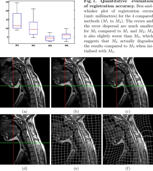
The box-and-whisker plot in Fig. 1 computed from the ten patients shows our algorithm (M3) to significantly outperform both M1(paired t-test: p = 3×10⁻⁴)
and M2(paired t-test: p = 2 × 10⁻³), with much smaller error and much smaller
error dispersal. M3 is also slightly better than M4(paired t-test: p = 5 × 10⁻²).
This suggests that the log-domain diffeomorphic demons performs worse than our algorithm even when properly initialised (using M3 instead of M1). The
results of M1, M2 and M3 on one of the ten patients are shown in Fig. 2, and
Fig. 1. Quantitative evaluation of registration accuracy. Box-and-whisker plot of registration errors (unit: millimetres) for the 4 compared methods (M1 to M4). The errors and
the error dispersal are much smaller for M3 compared to M1 and M2; M4
is also slightly worse than M3, which
suggests that M4 actually degrades
the results compared to M3 when
ini-tialised with M3.
(a) (b) (c)
(d) (e) (f)
Fig. 2. Registration results on a patient with flexion/neutral positions. (a) reference image; (d,b,c) floating image registered to the reference image with M1, M2,
M3 respectively; (e,f) same as (b,c) with deformation grids overlaid. The intersection
between the green and red lines shows the large error of M2 on the mandible; on the
contrary, M3 correctly matches this point. The ability of M3 to recover the flexion is
further illustrated by the deformation grid: the deformation visually appears as near-rigid on the lower head and face, while it shows extension near the back of the neck and contraction near the front of the neck; on the contrary, the deformation grid shows that M2 outputs near rigid movement everywhere.
4
Conclusion & Perspectives
It appears that our strategy for non-rigid registration, based on the computation of locally optimal rigid transformations in the first place, allows us to recover
(b) (c) (d)
(a)
(e) (f) (g)
(h)
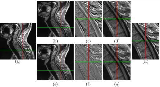
Fig. 3. Registration results on a patient with MS lesions in the spinal cord. (a) patient image at time point t0; (b) patient image at time point t1 registered with
M1and (e) with M3; (d,g) zoom on (b,e); (h) zoom on (a); (c,f) zoom on the difference
(registered minus reference) image. Note that in this case M2(not displayed) performs
as well as M3. These snapshots, and in particular the zoomed difference images, visually
show that M3gives a better result than a simple global rigid registration.
displacements and deformations of piecewise rigid structures (as seen e.g. in dynamic cervical MRI) much better than standard methods which are implic-itly based on locally optimal translations, such as the log-domain diffeomorphic demons algorithm. This original strategy was made possible by (i) the use of an up-to-date very efficient optimiser and (ii) the design of a specific regularising procedure on the (sparse) set of locally estimated rigid transformations, based on robust estimation techniques. A future line of research could be to combine our regularisation technique with those previously proposed in this context [9–11]. Our intuition is also that our algorithm could perform very well in more gen-eral problems, without necessarily rigid structures involved, and on other image modalities; we will evaluate this in a near future.
Acknowledgments. We thank ´Elise Bannier, Jean-Yves Gauvrit and Aurore Esquevin (CHU, University Hospital of Rennes, F-35043 Rennes, France) for discussions on the clinical protocol and for acquiring the MR images. We also thank Charles Kervrann (INRIA, SERPICO Project, F-35042 Rennes, France) for last-minute and life-saving reading suggestions.
References
1. Okuda, D., Mowry, E., Cree, B., Crabtree, E., Goodin, D., Waubant, E., Pelletier, D.: Asymptomatic spinal cord lesions predict disease progression in radiologically
isolated syndrome. Neurology 76(8) (2011) 686–692
2. Abitbol, J.J., Hong, S.W., Khan, S., Wang, J.C.: Dynamic MRI of the spine. In Szpalski, M., Gunzburg, R., Rydevik, B.L., Huec, J.C., Mayer, H.M., eds.: Surgery for Low Back Pain. Springer (2010) 39–45
3. Maintz, J., Viergever, M.: A survey of medical image registration. Med Image Anal 2(1) (1998) 1–36
4. Little, J., Hill, D., Hawkes, D.: Deformations Incorporating rigid structures. Com-put Vis Image Und 66(2) (1997) 223–232
5. Arsigny, V., Commowick, O., Ayache, N., Pennec, X.: A Fast and Log-Euclidean Polyaffine Framework for Locally Linear Registration. J Math Imaging Vis 33(2) (2009) 222–238
6. Commowick, O., Arsigny, V., Isambert, A., Costa, J., Dhermain, F., Bidault, F., Bondiau, P.Y., Ayache, N., Malandain, G.: An efficient locally affine framework for the smooth registration of anatomical structures. Med Image Anal 12(4) (2008) 427–441
7. Seiler, C., Pennec, X., Reyes, M.: Geometry-Aware Multiscale Image Registration via OBBTree-Based Polyaffine Log-Demons. In Fichtinger, G., Martel, A., Peters, T., eds.: MICCAI’2011. Vol. 6892 of LNCS, Springer (2011) 631–638
8. Rohlfing, T., Maurer, C.: Intensity-based non-rigid registration using adaptive multilevel free-form deformation with an incompressibility constraint. In Niessen, W., Viergever, M., eds.: MICCAI’2001. Vol. 2208 of LNCS, Springer (2001) 111– 119
9. Loeckx, D., Maes, F., Vandermeulen, D., Suetens, P.: Nonrigid image registra-tion using free-form deformaregistra-tions with a local rigidity constraint. In Barillot, C., Haynor, D., Hellier, P., eds.: MICCAI’2004. Vol. 3216 of LNCS, Springer (2004) 639–646
10. Ruan, D., Fessler, J.A., Roberson, M., Balter, J., Kessler, M.: Nonrigid registration using regularization that accomodates local tissue rigidity. In Reinhardt, J.M., Pluim, J.P., eds.: Medical Imaging 2006: Image Processing, SPIE Press (2006) 11. Staring, M., Klein, S., Pluim, J.P.: A rigidity penalty term for nonrigid registration.
Med Phys 34(11) (2007) 4098–4108
12. Taquet, M., Macq, B., Warfield, S.: Spatially Adaptive Log-Euclidean Polyaffine Registration Based on Sparse Matches. In Fichtinger, G., Martel, A., Peters, T., eds.: MICCAI’2011. Vol. 6892 of LNCS, Springer (2011) 590–597
13. Vercauteren, T., Pennec, X., Perchant, A., Ayache, N.: Symmetric log-domain diffeomorphic registration: A demons-based approach. In Metaxas, D., Axel, L., Fichtinger, G., Sz´ekely, G., eds.: MICCAI’2008. Vol. 5241 of LNCS, Springer (2008) 754–761
14. Powell, M.: The BOBYQA algorithm for bound constrained optimization with-out derivatives. Technical report, Centre for Mathematical Sciences, University of Cambridge, UK (2009)
15. Mrazek, P., Weickert, J., Bruhn, A.: On robust estimation and smoothing with spatial and tonal kernels. In Klette, R., Kozera, R., Noakes, L., Weickert, J., eds.: Geometric Properties for Incomplete data. Springer (2006) 335–352
16. Ourselin, S., Roche, A., Prima, S., Ayache, N.: Block Matching: A General Frame-work to Improve Robustness of Rigid Registration of Medical Images. In Delp, S., DiGioia, A., Jaramaz, B., eds.: MICCAI’2000. Vol. 1935 of LNCS, Springer (2000) 557–566