Collective behavior over social networks with data-driven and machine learning models

Collective Behavior over Social Networks with

Data-driven and Machine Learning Models

by

Yan Leng

B.S., Beijing Jiaotong University (2013)

M.S., Massachusetts Institute of Technology (2016)

Submitted to the Program in Media Arts and Sciences,

School of Architecture and Planning

in partial fulfillment of the requirements for the degree of

Doctor of Philosophy in Media Arts and Sciences

at the

MASSACHUSETTS INSTITUTE OF TECHNOLOGY

May 2020

c

○ Massachusetts Institute of Technology 2020. All rights reserved.

Author . . . .

Program in Media Arts and Sciences,

School of Architecture and Planning

May 5, 2020

Certified by . . . .

Alex Pentland

Professor of Media Arts and Science, MIT

Toshiba Professor

Thesis Supervisor

Accepted by . . . .

Tod Machover

Academic Head, Program in Media Arts and Sciences

Collective Behavior over Social Networks with Data-driven

and Machine Learning Models

by

Yan Leng

Submitted to the Program in Media Arts and Sciences, School of Architecture and Planning

on May 5, 2020, in partial fulfillment of the requirements for the degree of

Doctor of Philosophy in Media Arts and Sciences

Abstract

Individuals form network connections based on homophily; individuals’ networks also shape their actions. Pervasive behavioral data provides opportunities for a richer view of the decisions on networks. Yet, the increasing volume, complex structures, and dynamics of behavioral data stretch the limit of conventional methods. I develop mathematical modeling (e.g., machine learning, game theory, and network science) and large-scale behavioral data to study collective behaviors over social networks. My dissertation will tackle this area in four directions, revolving around the intricate linkage between individuals’ characteristics, actions, and their networks. First, I empirically investigate how social influence spreads over networks using two massive cell phone data, and theoretically model how do individuals aggregate information from local neighbors. Second, I study how to leverage influential nodes for selective network interventions (e.g., marketing and political campaigns), by proposing a centrality measure going beyond network structures. Third, I build a geometric deep learning model to infer individual preferences and make personalized recommendations to utilize noisy network information and nodal features effectively. Last, given that the network is essential, I develop a framework to infer the network connections based on observed actions, when networks are unavailable. My thesis provides building blocks for further network-based machine learning problems integrating nodal heterogeneity and network structures. Moreover, the findings on human behaviors and frameworks developed in my thesis shed light on marketing campaigns and population management.

Thesis Supervisor: Alex Pentland

Title: Professor of Media Arts and Science, MIT Toshiba Professor

Acknowledgments

I am extremely fortunate to have interacted with and learned from so many amazing individuals, without whom my academic journey would not have gone this far. This acknowledgment only touches the surface.

First and foremost, I am indebted to my advisor Alex ‘Sandy’ Pentland, who has been extremely helpful for my professional development. His vision, wisdom, creativity, enthusiasm, and professionalism have been constant sources of inspiration ever since the day I took the courage to email him. Sandy is an incredibly supportive and down-to-earth advisor. Whenever I bounced ideas with him, he can always connect the dots and shape my immature idea in a more prom ming direction.

I am also grateful to my committee member, Dean Eckles. Every time I interact with Dean, I learn something new. Dean is extremely well-read and knowledgeable. His infectiously cheerful personality and his generosity with his time have been hugely helpful for me. I look up to him for his passion for social network and dedication to causal inference.

I am grateful for my committee member, Esteban Moro. Esteban has been an excellent collaborator and committee member: his insights have had a significant influence over my research, and it was his generous encouragement that got me finished my first project of in Ph.D. Esteban has also been a great mentor. His professionalism has hugely influenced and will continue to affect my academic career.

I am also grateful and fortunate to have Michael Bronstein in my committee. It was his seminal work on deep geometric learning that introduced me to this field. I am grateful for Michael’s generosity of time and inspiring discussions on ideas. I look forward to continuing to learn from him and collaborate more in the future.

I am also indebted to my former advisors, Haris Koutsopolous, Jinhua Zhao, Larry Rudolph, and Xuedong Yan, who took me as a research assistant, introduced me to transportation and mobility research and provided continual support before I start Ph.D.

with the ideal environment for interdisciplinary research. I have learned from many other faculty members and students here. I have been so fortunate to have interacted with faculties from different departments to learn from their expertise. I would like to especially thank Kent Larson for allowing me to join the Andorra project, where I meet many passionate researchers with different expertise.

I wouldn’t have survived graduate school without my wonderful peers. There are so many people I should extend my gratitude. My close collaborator, Xiaowen Dong, taught me a lot about research and is always there as a close friend. My office mates, Abdullah Almaatouq and Alejandro Noriega, always impressed me with their positivity and passion for making a societal impact. I am lucky to have Morgan Frank and Mohsen Mosleh, who I chatted a lot to go through the stressful time on the job market. I am also fortunate to have Michiel Bakker as a good friend, whose sense of humor has influenced me a lot. I would also like to thank my lab mates Yuan Yuan, Mohsen Bahrami, Zivvy Epstein, Eaman Jahani, Dhaval Adjodah, Tara Sowriraja, Dan Calacci, Martin Saveski, for our discussion of ideas and for friendships that made my overall graduate school experience.

Finally, I want to express my deep and sincere gratitude to my family for their continuous and unparalleled love, help, and support. As the only child, my parents always try to give me the best they can offer. It is their encouragement and sacrifice that take me this far. Last but not least, I want to thank my husband, Siyuan Liu. Siyuan is not only my partner but also a role model that I always look up to. Meeting you is the best part of my graduate school, and you excel in every part of our life.

This doctoral thesis has been examined by the following committee

members:

Professor Alex ‘Sandy’ Pentland . . . .

Thesis Supervisor

Professor of Media Arts and Science, MIT

Toshiba Professor

Media Lab Entrepreneurship Program Director

Professor Michael Bronstein. . . .

Thesis Committee

Professor at the Department of Computing, Imperial College London

Professor Dean Eckles . . . .

Thesis Committee

KDD Career Development Professor in Communications and Technology

Associate Professor of Marketing at MIT Sloan School of Management

Professor Esteban Moro . . . .

Thesis Committee

Visiting Professor, MIT Media Lab

Associate Professor at the Universidad Carlos III de Madrid

Contents

1 Introduction 25

1.1 Background . . . 26

1.2 Research questions . . . 27

2 Long range social influence in phone communication network 31 2.1 Introduction . . . 32

2.2 Literature review . . . 35

2.2.1 Contagion models . . . 35

2.2.2 Observational learning and word-of-mouth effect . . . 36

2.3 Behavioral matching framework . . . 36

2.3.1 Setting . . . 37

2.3.2 Matching framework . . . 40

2.4 Long range of social influence . . . 42

2.5 Bayesian learning model and results . . . 48

2.5.1 Bayesian learning model . . . 48

2.5.2 Comparisons between the Bayesian learning model with existing models . . . 52

2.5.3 Prediction results . . . 53

2.6 Managerial implications . . . 54

2.7 Discussion . . . 55

3 Contextual centrality: going beyond network structure 61 3.1 Introduction . . . 62

3.2 Contextual centrality . . . 64

3.3 Results . . . 69

3.3.1 Methods . . . 69

3.4 Discussion . . . 79

3.5 Properties of contextual centrality . . . 81

3.5.1 Bounds and distribution of contextual centrality in terms of spreadability . . . 81

3.5.2 Robustness of contextual centrality in response to perturbations in y . . . 82

3.5.3 Theoretical results of contextual centrality for Erdos-Renyi net-works . . . 84

3.5.4 The relationship between contextual centrality and other cen-trality measures . . . 90

3.5.5 Relationship between approximated cascade payoff and cascade payoff . . . 92

3.5.6 Game-theoretic interpretation of contextual centrality with local interactions . . . 92

3.5.7 Differences between contextual centrality and centrality mea-sures developed on weighted networks . . . 94

3.6 Additional results for empirical analysis . . . 96

3.6.1 Predictive power of contextual centrality in eventual adoptions 96 3.6.2 Performance relative to other centrality measures on random networks . . . 98

3.6.3 Average approximated cascade payoff for contextual centrality and the variations of other centrality measures . . . 102

3.6.4 Comparison of seeding strategies when y(U𝑇₁y) < 0 . . . 104

4 Recommender systems with heterogeneous information: A geomet-ric deep learning approach 107 4.1 Introduction . . . 108

4.2 Literature review . . . 113

4.2.1 Recommender systems . . . 113

4.2.2 Geometric deep learning . . . 114

4.3 Data description . . . 116

4.3.1 Business . . . 116

4.3.2 Users . . . 118

4.4 Model . . . 120

4.4.1 Problem formulation . . . 121

4.4.2 Local smoothness regularization with graph attention network 122 4.4.3 Framework . . . 125

4.5 Results . . . 127

4.5.1 Experimental setting . . . 127

4.5.2 Learning performance . . . 129

4.5.3 Pattern analysis on business representations . . . 132

4.6 Conclusion and managerial implications . . . 135

5 Learning Quadratic Games on Networks 139 5.1 Introduction . . . 140

5.2 Network games of linear-quadratic payoffs . . . 142

5.3 Learning games with independent marginal benefits . . . 145

5.3.1 Learning framework . . . 145

5.3.2 Learning algorithm . . . 147

5.4 Learning games with homophilous marginal benefits . . . 147

5.4.1 Learning framework . . . 148

5.4.2 Learning algorithm . . . 149

5.5 Experiments on synthetic data . . . 149

5.5.1 Comparison of learning performance . . . 151

5.5.2 Learning performance with respect to different factors in network games . . . 152

5.6 Experiments on real world data . . . 154 5.6.1 Social network . . . 155 5.6.2 Trade network . . . 155 5.7 Discussion . . . 157 6 Conclusion 165 6.1 Summary . . . 165 6.2 Future work . . . 169

A Interpretable Stochastic Block Influence Model: measuring social influence among homophilous communities 187 A.1 Introduction . . . 188

A.2 Related literature . . . 191

A.3 Methodology . . . 192

A.3.1 Stochastic Block Influence Model . . . 192

A.3.2 Generative process . . . 195

A.4 Experiments . . . 198

List of Figures

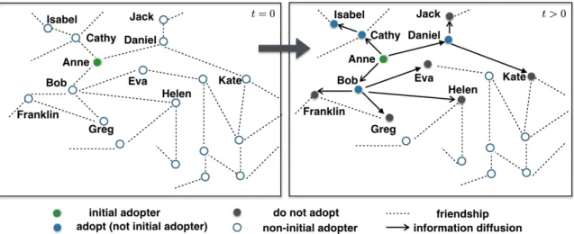
2-1 An illustration of initial adopters, information cascade, and the hop indexes. In the information cascade 𝒞𝑇 shown in the figure,

within an observation period 𝑇 , the initial adopter Anne (colored green) passes information to her neighbors, Bob, Eva, Cathy, and Daniel, who after receiving information from Anne continue to pass the information onwards. Labeled with hop index one, they further diffuse the information to Franklin, Greg, Helen, Isabel, Jack, and Kate, who are then on hop index two. The process continues until the end of the observation period. Among the people who receive information, Bob, Isabel, and Daniel (colored blue) decided to adopt the behavior, while others (colored grey) decided not to. . . 40

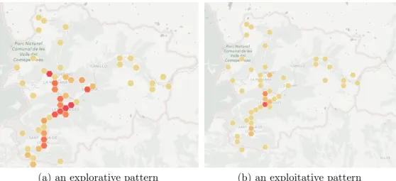
2-2 Two types of mobility frequency patterns during weekends, revealing different individual preferences: (a) an explorative pattern; (b) an exploitative pattern. The intensity of the color represents the normalized visitation frequency, i.e., the darker red color corresponds to a more frequent visit. . . 41

2-3 Percentage improvement in adoption rate relative to the con-trol group due to social influence via phone communication network (Δ𝐴ℎ): (a) attending cultural performance; (b) visiting the

retail store. The y-axis is the difference in adoption likelihood of the two groups, and the x-axis is the hop index. The purple, blue, and red dashed lines show the estimated effect of social influence using PSM, random matching, and PSM after a shuffling test, respectively. The shaded regions correspond to the 5% and 95% confidence intervals from bootstrap sampling. The higher and lower end of the vertical line indicates the 5% and 95% interval. . . 44 2-4 Matching on behavioral covariates, and on both behavioral

covariates and socio-demographics, for the adoption behavior of visiting the retail store. The y-axis is the difference in adoption likelihood of the two groups, and the x-axis is the hop index. The bar plot and the vertical lines correspond to the mean, 5%, and 95% confidence intervals, respectively. The blue and red bars correspond to behavioral matching, and behavioral + socio-demographics matching. 45 2-5 SMD for the matching between the control group and the

different treatment groups (different hop indexes ℎ), in the case of attending cultural performance. . . 46 2-6 SMD for the matching between the control group and the

different treatment groups (different hop indexes ℎ), in the case of visiting retail store. . . 47 2-7 Percentage improvement in adoption rate relative to the

con-trol group due to social influence estimated by post-Lasso logistic regression for different treatment groups (Δ𝐴ℎ), in the

case of a) attending cultural performance and b) visiting the retail store. The vertical bars cover 5% and 95% confidence intervals. . . 48

2-8 Decision-making process for Greg, according to the proposed Bayesian learning model. At the time instance 𝑡 = 0, Greg forms a prior understanding of the product. At 𝑡 = 1, Bob told Greg about his evaluation of the product. Knowing Bob’s general preference, Greg then updated his perception (𝑃1(𝑤Greg)). The same updating process

happens after observing the preferences and the evaluations of Franklin and Helen afterward. With this illustration, we show how Greg updates his perception about the product by dynamically aggregating local information from his neighbors who communicated with him. . . 51

2-9 Higher-order social influence. Existing contagion models assume that individual behaviors are independent of the decisions of others conditioned on their immediate neighbors. That is to say, existing contagion models do not distinguish scenarios A and B in terms of the decision-making of Greg. Our model, thanks to the higher-order social influence and propagation of information between neighbors, can separate the two scenarios. . . 53

2-10 Performance of different models in predicting adoption be-havior: (a) attending cultural performance; (b) visiting retail store. The error bars correspond to the 5% and 95% confi-dence intervals. . . 54

2-11 Percentage of individuals (a,c) as well as their adoption rates (b,d) at each hop, computed using information cascades from

3-1 Predictive power of contextual centrality. We show how the average centrality of first-informed individuals predicts the eventual adoption rate of non-first-informed individuals in (a) microfinance and (b) weather insurance. The y-axis shows the 95% confidence interval of 𝑅2 computed from 1000 bootstrap samples from ordinary least squares regressions controlling for village size. The x-axis shows varying values for 𝑝𝜆1, which influences only diffusion

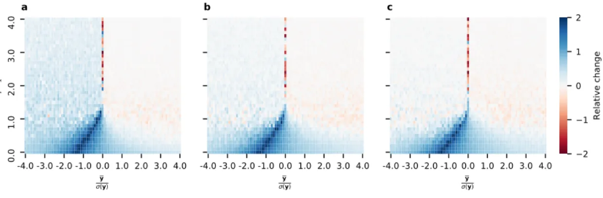
centrality and contextual centrality. . . 72 3-2 Performance of contextual centrality relative to other

central-ity measures on random networks. Each plot shows the relative change, computed as _{max(|𝑎|,|𝑏|)}𝑎−𝑏 where 𝑎 is CC’s average payoff and 𝑏 is the maximum average payoff of the other centrality measures, for varying values of _𝜎(y)y and 𝑝𝜆1. The plots correspond to the results on

random networks generated according to the (a) Barabasi-Albert, (b) Erdos-Renyi, and (c) Watts-Strogatz models. . . 74 3-3 Average payoffs when standardized average contribution is 0.

Here we show the average payoff with 95% confidence interval when seeding with different methods on (a) Barabasi-Albert, (b) Erdos-Renyi, and (c) Watts-Strogatz models. . . 75 3-4 Average payoffs when standardized average contribution is 1.

Here we show the average payoff with 95% confidence interval when seeding with different methods on (a) Barabasi-Albert, (b) Erdos-Renyi, and (c) Watts-Strogatz models. . . 76 3-5 Performance of contextual centrality relative to other

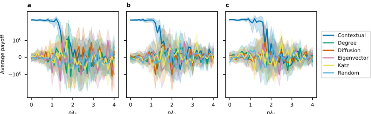
central-ity measures on real-world networks, including (a) microfi-nance, (b) weather insurance, and (c) political campaign. Each plot shows the relative change for varying values of 𝑝𝜆1. We compare

contextual centrality with degree centrality, diffusion centrality, eigen-vector centrality, Katz centrality, and random seeding. . . 77

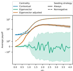
3-6 Average cascade payoff for variations of contextual centrality and eigenvector centrality. The x-axis is 𝑝𝜆1, and the y-axis

is the average payoff, with the shaded region as the 95% con-fidence interval. For “eigenvector adjusted” centrality, we multiply eigenvector centrality with the primary contribution U𝑇₁y. For “seed nonnegative”, we only seed if the maximum of the centrality measure is nonnegative, otherwise it is named “seed always”. . . 78

3-7 Homophily and maximum of contextual centrality when 𝑝𝜆1 <

1. We regress the maximum of contextual centrality on homophily after controlling for _𝜎(y)y and 𝑝𝜆1. The y-axis is the OLS coefficients of

homophily (with the vertical line as the 95% confidence interval) and the x-axis corresponds to three types of networks. We perform the analysis separately for _𝜎(y)y being larger than, smaller than and equals to zero. . . 79

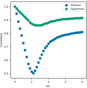
3-8 Relationship between approximated cascade payoff and cas-cade payoff. The y-axis and x-axis display the correlation and the spreadability ( 𝑝𝜆1) respectively. Pearson and Spearman’s correlation

are shown in blue and orange color respectively. . . 93

3-9 Predictive power of contextual centrality without any controls for (a) microfinance and (b) weather insurance. The y-axis shows the 95% confidence interval of 𝑅2 _{computed from 1000 bootstrap}

samples from ordinary least squares regressions controlling for village size. The x-axis shows varying values for 𝑝𝜆1, which influences only

3-10 Predictive power of contextual centrality with additional con-trols for (a) microfinance and (b) weather insurance. For (a), we use village size, savings, self-help group participation, fraction of general caste members, and the fraction of village that is first-informed as done in [23]. For (b), we use village size, number of first-informed households, and fraction of village that is first-informed. The y-axis shows the 95% confidence interval of 𝑅2 computed from 1000 bootstrap samples from ordinary least squares regressions controlling for village size. The x-axis shows varying values for 𝑝𝜆1, which influences only

diffusion centrality and contextual centrality. . . 97 3-11 Average payoffs with 95% confidence interval when

standard-ized average contribution is -4 for (a) Barabasi-Albert, (b) Erdos-Renyi, and (c) Watts-Strogatz models. . . 98 3-12 Average payoffs with 95% confidence interval when

standard-ized average contribution is -3 for (a) Barabasi-Albert, (b) Erdos-Renyi, and (c) Watts-Strogatz models. . . 99 3-13 Average payoffs with 95% confidence interval when

standard-ized average contribution is -2 for (a) Barabasi-Albert, (b) Erdos-Renyi, and (c) Watts-Strogatz models. . . 99 3-14 Average payoffs with 95% confidence interval when

standard-ized average contribution is -1 for (a) Barabasi-Albert, (b) Erdos-Renyi, and (c) Watts-Strogatz models. . . 99 3-15 Average payoffs with 95% confidence interval when

standard-ized average contribution is 0 for (a) Barabasi-Albert, (b) Erdos-Renyi, and (c) Watts-Strogatz models. . . 100 3-16 Average payoffs with 95% confidence interval when

standard-ized average contribution is 1 for (a) Barabasi-Albert, (b) Erdos-Renyi, and (c) Watts-Strogatz models. . . 100

3-17 Average payoffs with 95% confidence interval when standard-ized average contribution is 2 for (a) Barabasi-Albert, (b) Erdos-Renyi, and (c) Watts-Strogatz models. . . 100 3-18 Average payoffs with 95% confidence interval when

standard-ized average contribution is 3 for (a) Barabasi-Albert, (b) Erdos-Renyi, and (c) Watts-Strogatz models. . . 101 3-19 Average payoffs with 95% confidence interval when

standard-ized average contribution is 4 for (a) Barabasi-Albert, (b) Erdos-Renyi, and (c) Watts-Strogatz models. . . 101 3-20 Average cascade payoff for variations of contextual centrality

and degree centrality. . . 102 3-21 Average cascade payoff for variations of contextual centrality

and diffusion centrality. . . 103 3-22 Average cascade payoff for variations of contextual centrality

and katz centrality. . . 103 3-23 Comparison of seeding strategies when y(U𝑇₁y) < 0 for (a)

continuous and (b) discrete. . . 105

4-1 Motivating example. Each individual is characterized by hobbies and educational background. The black and green link correspond to professional and social networks, respectively. . . 111 4-2 Predicting customer preferences on businesses as a matrix

completion task. . . 112 4-3 Distributions of average ratings of businesses and users. . . 117 4-4 Spatial distributions of businesses and users. The spatial

location of a user is the weighted average location of the businesses she has reviewed. The color code represents the average ratings of businesses and users. . . 119

4-5 Relationship between spatial distance, difference in average rating, cosine distance between the business attribute vector, and cosine distance between the check-in time vector. The middle line, lower and upper boundaries of the box (interquartile range or IQR) correspond to mean, median, 25% and 75% of the data, respec-tively. The lower and upper whiskers extend maximally 1.5 times of IQR from 25 percentile downwards and 75 percentile upwards, respectively. 120 4-6 The count of user pairs, difference in average rating, and

co-sine distance between the user metadata vector, concerning the degrees of separation in the Yelp friendship network. The middle line, lower and upper boundaries of the box (interquartile range or IQR) correspond to mean, median, 25% and 75% of the data, respec-tively. The lower and upper whiskers extend maximally 1.5 times of IQR from 25 percentile downwards and 75 percentile upwards, respectively. 121 4-7 Basic idea behind a graph attention network. The attention

weight 𝛼𝑖𝑗 represents the relevance of neighbor 𝑣𝑗 in updating

informa-tion on 𝑣𝑖. . . 125

4-8 The proposed geometric deep learning architecture for learn-ing latent user representations 𝑈 and business representations 𝑉 , via iterations over three layers: a dense layer, an LTSM layer, and a GAT layer. The predicted ^𝑋 is obtained using the final updates of 𝑈 and 𝑉 via ^𝑋 = 𝑈 𝑉𝑇_{. . . . 127}

4-9 Distribution of attention weights. . . 131 4-10 Attention weights for a focal (a) user and (b) business. Nodes

are colored by average rating of the user or business, and the intensity of a link represents the attention weight. . . 131 4-11 Regression coefficients with confidence intervals for

4-12 Analysis of business categories of different business clusters in Cleveland Heights. The relative sizes of the words correspond to the frequencies of the category. . . 135 4-13 Analysis of business categories of different business clusters in

Urbana. The relative sizes of the words correspond to the frequencies of the category. . . 135 5-1 Performance of the proposed algorithm and baselines in the

setting of independent (top) and homophilous (bottom) marginal benefits. The red triangle, the middle line, lower and upper boundaries of the box (interquartile range or IQR) correspond to mean, median, and 25/75 percentile of the data, respectively. The lower and upper whiskers extend maximally 1.5 times of IQR from 25 percentile downwards and 75 percentile upwards, respectively. . . 151 5-2 Performance of Algorithm 3 versus structural properties of

the network. . . 153 5-3 Performance (AUC) of Algorithm 2 with respect to 𝜌(𝛽G), 𝜃1,

and 𝜃2. . . 160

5-4 Performance (AUC) of Algorithm 3 with respect to 𝜌(𝛽G), 𝜃1,

and 𝜃2. . . 161

5-5 Performance of Algorithm 3 versus number of games (top) and noise intensity in marginal benefits (bottom). . . 162 5-6 Performance of Algorithm 3 versus strength of homophily in

the marginal benefits. . . 162 5-7 Performance of Algorithm 2 versus number of games (top),

noise intensity in marginal benefits (middle), and structural properties of the network (bottom). . . 163 5-8 Clustering of Swiss cantons based on the political network

A-1 Graphical representation of the Stochastic Block Influence Model (SBIM). Assume there are two communities, a high socioeco-nomic status (SES) group (colored in dark blue) and low SES group (colored in dark red), characterized by multi-dimensional

sociodemo-graphic features. The two groups have higher intra-class connection probability and lower inter-class connection probabilities. The decision-making of A is jointly influenced by her preferences, as well as her neighbors from the same and different communities. . . 196 A-2 Size of each social block. The y-axis corresponds to the number of

individuals in the block, and the x-axis is the corresponding block index.201 A-3 Adjacency matrix sorted by the inferred block index. The x-axis and

y-axis correspond to the indices of individuals. The white and black cells correspond to the existence and the non-existence of edges. We can clearly observe the underlying communities from the network. . . 203 A-4 Interaction matrix and influence matrix. . . 208 A-5 Sociodemographic analysis of each social block and the social

influence across social blocks. Each node represents a social block corresponding to the index shown in the previous in Table A.2. The directed links represent the strength of social influence varying from strong negative (blue) to strong positive (red). The color of the node represents a measure of the sociodemographic characteristics within that social block. We display a subset of characteristics, including median age, gender ratio, caste diversity, language diversity, and profession diversity within each block. . . 209

List of Tables

2.1 Basic statistics about the mobile phone data set in country A. 38 2.2 Basic statistics about the mobile phone data set in the city in

country B. . . 38

3.1 Centrality measures defined by c𝑡= 𝛼Ac𝑡−1+ 𝛽. . . 91

4.1 Summary statistics of the data. . . 116 4.2 Notations . . . 123 4.3 Performance comparison using RMSE metric (standard errors

in parentheses). . . 129 4.4 Cluster characteristics for Cleveland Heights (C.H.) and

Ur-bana (U.). . . 134

5.1 Performance (𝑅2_{) of learning marginal benefits. . . . . 154}

5.2 Performance (AUC) of learning the structure of the social network and the trade network. . . 156

A.2 Block characteristics example. SES is an abbreviation for socioeconomics status. The majority refers to the largest subset. Disadvantaged caste refers to lower castes, including the castes OBC (Other Backward Class) and Scheduled. Higher education refers to having education levels at PUC (pre-university course) and having a “degree or above” designation. Moderate and lower education levels include all levels below this, where moderate levels have more SSLC (Secondary School Leaving Certificate) levels, and PUC levels and lower

levels have mostly primary school education levels. . . 204 A.3 Block attributes associated with different types of influence.

Positive and negative influence refers to the type of influence from one block to another block. Self-influence refers to positive influence within the same block. Overlap refers to overlapping categories, such as caste type, profession type, education levels, or languages spoken. . . 205

Chapter 1

Introduction

Telescope and microscope are two revolutionary technologies in astronomy and biology. They enable human beings to see things that are invisible to naked eyes, either is too small or too far away. The capabilities to collect and analyze massive amounts of data dramatically change these fields. A similar revolution is currently taking place in social science. Digital technologies are similar to telescope and microscope and are named as “socioscope” [161]. They enable researchers to collect information about human behavior that are invisible through lab experiments and surveys. They capture information about apps we use, the places we travel to, people we interact with, and transactions we make. The large-scale, high-resolution, longitudinal, and dynamic information enables us to ask a much broader set of questions on human behaviors, which are not possible through traditional lab experiments and surveys. Yet, the increasing volume, complex structures, and dynamics of behavioral data, as well as the research questions on the complicated human interactions, stretches the limit of conventional methods. The emerging field of data-driven “Computational Social Science” is sparked by the massive amounts of digital records of human behaviors [128]. Before 2000, research on human interactions relied heavily on or one-shot and self-reported data, and data on rational decisions were mostly collected via surveys or lab experiments. Even though lab experiments allow precise control of extraneous variables—making it easier to establish causal relationships and understand the underlying mechanism, the artificial setting makes it difficult to generalize to real

life.

With digital technologies, researchers can perform observational studies with passively collected data sets—such as mobile phone records, credit card transactions, or social media data—on a large-scale (more representative comparing with traditional data collections) population and in a dynamic fashion. New technologies offer at least three advantages. First, the data provides much higher resolution information both at a temporal and spatial scale, including granular information about user behaviors and individuals connections. This enables us to understand the underlying mechanism for the human decision-making process and design interventions accordingly. Second, digital technologies enable us to have a more comprehensive picture of how a ’macro’ social network performs, including human behaviors at a city scale for an extended period. Third, digital platforms capture information dynamically, enabling us to understand how society evolves.

1.1

Background

Collective behavior over social networks It is a widely-known phenomenon in social science that collective behavior is not simply adding up individual behavior; because individuals interact. They learn from, strategically interact with, exert peer pressure on each other. At the same time, the social norm emerges. The social network is interesting not only because it influences how decisions are made; but also because of the rich information contained in the interactions. On the one hand, no decision is made in isolation. Specifically, social influence leads to associations in decisions among neighbors and can help organizations to spread products and policy-makers for population management. On the other hand, not merely a medium to connect people, social networks also contain rich information about individuals due to the endogenous network formation and the dependencies in decision-making. The investigation of human behaviors over social networks enables us to understand a wide range of domains, including innovations, competing technologies, cultural fads, social norms, cooperation, social disorder, or financial markets. Hence, how decisions are

made in a network environment has raised interests and has overarching applications in such diverse fields as sociology, economics, health, and political science [14, 23, 63, 44].

A need for new computational tools to deal with the complexities in both human decision-making and the behavioral data structures. The perplexi-ties in human behavior and the increasingly complicated data structures stretch the limits of traditional methods, e.g., data analysis and research designs. There is a need for new computational techniques to understand, predict, and intervene in human decisions, in response to the rich and heterogeneous behavioral information. More recently, technological advances networks facilitate social interactions that otherwise would not take place. These social interactions, therefore, raise many fundamental questions, such as how social influence change short-term decision-making and long-term habits, how do individuals make strategic decisions in a networked environment, how can organizations incentivize behavioral changes by leveraging network effect.This thesis will tackle these questions with new computational methods and large-scale datasets.

1.2

Research questions

My thesis answers questions related to how social influence affects decision-making, how to leverage essential individuals for network-based interventions, how to pre-dict preferences using network information, and how to recover networks based on individuals’ actions. To achieve this, I develop tools to integrate individual ratio-nal decision-making and machine learning to help with learning problems on social interactions. I will describe the research questions in more detail as follows.

How does social influence spread over social networks? How does the information aggregation process influence the diffusion of social influence? Several empirical studies have shown that social influence propagates beyond direct neighbors is relatively costless online decision-making settings. Yet, precisely how influence plays a role in costly offline behaviors and spreads through a social network

remains unclear. I leverage the high-resolution mobile phone data and a new behavioral matching framework to study how social influence propagates and affects individual offline behavior. The results show that propagation within the network persists in shaping individual decisions through up to three degrees of separation. To further understand the diffusion of social influence on offline adoption decisions, I propose a Bayesian learning model based on local information aggregation, which better predicts individual adoption behavior than exposure-based contagion models.

How can we design a centrality measure to incorporate both the network connections and the characteristics of individuals nodes? Existing centrality measures study the connectedness of individuals. However, these measures are less helpful in some applications where the objective is to target users who spread positive influence, such as viral marketing or political campaigns. I develop the "contextual centrality" to guide such applications. In particular, contextual centrality evaluates individuals’ importance based on network positions and nodal characteristics. It generalizes over existing centrality measures and provides insights on both local and global diffusion. Contextual centrality is shown to perform better in the empirical analysis and simulations on the marketing campaigns for microfinance and weather insurance in rural Indian and Chinese villages. This work provides building blocks for integrating network structures and note features in future network studies.

How to effectively integrate network connections and auxiliary informa-tion about individuals to extract informative network connecinforma-tions for the recommendation? Relative to the prior state-of-the-art recommender systems, which employed either nodal characteristics or network structure—but not both—for the recommendation, our approach enables recommendation systems to combine both sources of information to extract useful components of the network and predict indi-vidual preferences using data with a complex structure. I test the methodology to Yelp review data and predict customer preferences for restaurants they have not rated, utilizing information on historical ratings, socio-demographics, business characteristics,

check-in information, geographical information, and social networks. The methodology has a wide range of other potential applications, including behavioral predictions and preference inference.

How can we infer the network connections from observed actions when the networks are unavailable? In many social settings, social connections are either unobserved or noisily measured. Individual actions provide information about the underlying interaction structures due to the dependencies of neighbors’ actions. I formalize this idea with a linear-quadratic network game. This game is an approxima-tion of all static games with continuous utility funcapproxima-tions. I use Nash Equilibrium to approximate users’ actions by assuming that rational agents maximize their utilities. I provide conditions under which network structure can be inverted from observed actions, and I perform several empirical applications of the framework.

Chapter 2

Long range social influence in phone

communication network

Several empirical works have shown that, in online decision-making settings, social influence propagates beyond direct contacts, mainly due to the exposure effect ex-plained by simple or complex contagion [96, 59, 44, 80, 16]. Yet precisely how influence affects offline behaviors and propagates through a social network, and especially the underlying mechanism that drives such propagation, remain unclear [66, 172, 44]. In this study, we leverage high-resolution mobile phone data sets and a new behavioral matching method based on revealed preference theory, to study how social influence propagates and affects individual off-line behavior. Our results show that propagation within the network persists in shaping individual decision-making to more than three degrees of separation regarding attending an international cultural performance in a European country and visiting a newly opened retail store in a city in North America. To better understand this long range effect of social influence, we propose a Bayesian learning model based on a local learning and information aggregation process, and show that it leads to better prediction of individual adoption behavior compared to exposure-based models. The present study contributes to a theoretical understanding of the diffusion of influence in social networks, which may have significant implications in a variety of practical domains. 1

2.1

Introduction

The effect of social influence on shaping individual decision-making, in various aspects of daily life, has attracted interest from such diverse fields as sociology, marketing, economics, health, and political science [64, 47, 23, 14, 63, 44]. One important motivation of studying social influence is that it may lead to an cascading effect: one’s action may influence their direct contacts, who further diffuse the influence through the contact network. Prominent contagion-based theories [96, 59] in social sciences explain the cascading patterns of such diffusion for certain behaviors, such as adopting an app [189, 13], expressing political preferences [44], or sharing a post on social media [125]. These theories model the adoption behaviors as an outcome of exposure to either a single source of information, such as disease spreading [196] and information spreading [19], or multiple sources of information [59], such as registration for health forum [58] and adoption of hashtags [165].

With the increasing popularity of online social networks, many studies have sought to empirically measure the diffusion of social influence on decision-making in virtual space. Notable examples include [44], which uses a 61-million-person online experiment to show that one’s political self-expression can be influenced by the friends of their friends; and [80], which uses public goods game in an online experiment to show that behavioral contagion reaches up to three degrees of separation in a social network. Moreover, [16] conducted a randomized experiment and shows that integrating viral features into commercial applications hosted on Facebook increases the total adoption, due to passive broadcasting messages spread through the Facebook network.

Comparing to the online setting, most studies of offline behavioral contagion, such as that of exercising activities [15], voting behavior [44], and adoption of microfinance [25], is restricted to direct neighborhood in the social network. On the one hand, offline behaviors are associated with a higher cost of communication and decision-making; hence, their diffusion is likely to have a broader socioeconomic impact. On the other hand, this presents significant challenges due to the difficulty in getting quality data for studying large-scale offline behaviors as well as that in measuring the effect of

social influence in such settings. The theory of "three degrees of influence" proposed by [64] is based on small-scale offline experiments focusing on smoking behavior, happiness, and habits that led to obesity, and found that they propagate within a social network up to three degrees of separation. However, the strategy in identifying social influence in their work has raised some criticism [172, 66], and the size and scale of the experiments are relatively limited.

To understand how influence on offline behaviors propagates in a large-scale social network, we leverage two high-resolution data sets of mobile phone communication records from the country A and the one city in Country B, to construct offline communication networks and study the effect of social influence on two types of offline adoption behaviors: i) attending an international cultural performance, and ii) visiting a newly opened retail store. We focus on the effect beyond direct contact or immediate neighbors in the communication network. To control for potential confounding factors such as homophily, we propose a novel matching framework to mimic the random assignment of treatment, conditioning on personal preference that is revealed by historical mobility patterns [133]. This framework allows us to study the propagation of influence in large-scale settings, thereby overcoming the difficulty of applying randomized controlled trials (RCTs) in such scenarios [28]. Our results show that, within the communication network, the effect of social influence decays from the initial adopters’ direct contacts but, surprisingly, persists to more than three degrees of separation in both cases. This result suggests that one’s decision to adopt and communicate with others may impact individuals in the network far beyond one’s direct contacts. Indeed, this pattern of social influence resembles the physical phenomenon of ripples expanding across the water when an object is dropped into it.

Traditional contagion-based models bear attractive mathematical properties and achieve good performance in predicting adoption behavior that is dominated by exposure. Going beyond simple exposure-based models, we are interested in the mechanism behind decision-making where rational individuals maximize their utilities by learning and aggregating information from neighbors in a social network [204]. More specifically, we propose a Bayesian learning model in which individuals dynamically

update their posterior beliefs towards the adoption behavior and make decisions on adoption based on the local information they collect from immediate neighbors. We further show the link between the proposed model and the empirical decaying pattern of the effect of social influence. In a task of predicting future adoption, the proposed model outperforms other state-of-the-art contagion models, including , the independent cascade model [116, 119], the threshold model [95, 195] and the structural econometric model [23], thereby suggesting the importance of incorporating the local information aggregation process into network-based Bayesian learning for predicting individual decision-making.

We make several contributions to the existing research. First, we leverage two large-scale mobile phone data sets to show that in a dynamic phone communication network the effect of social influence on offline decision-making can extend to more than three degrees of separation. This demonstrates the hidden impact of one’s decision on that of others beyond one’s immediate circle, which may be used for designing network-based intervention and marketing campaigns. Second, our research design can be generalized to study social influence in a wide range of online and offline settings with rich behavioral information. On the one hand, thanks to the availability of mobile phone data (i.e., call detail records) in almost every country in the world, such study becomes possible even when running large-scale experiments might be difficult due to resource constraint. On the other hand, we highlight the effectiveness of behavioral data in revealing users’ preferences and other characteristics such as socio-demographics. Behavioral information are not only more commonly-collected on digital platforms, but can also be studied in a dynamical fashion, hence capturing the potential change in users’ preferences and tastes. Third, we develop a Bayesian learning model which extends existing contagion models with a dynamic local information aggregation process. This extension accounts for individual heterogeneity and can capture both positive and negative influence signals. The improvement in the prediction performance achieved by the proposed Bayesian learning model demonstrates that the propagation of social influence is more complex in offline than online settings, which calls for the need for a decision-making mechanism that goes

beyond simple contagion or exposure-based models.

The rest of this section of my thesis is organized as follows. Section 4.2 presents a review of the literature. Section 2.3 describes the data used in this chapter, and proposes the behavioral matching strategy. Section A.4 presents the empirical results with robustness analysis, and section A.3 develops a Bayesian learning model with a local information aggregation process. Section 2.6 highlights managerial implications and Section 2.7 present discussion of the results of the study.

2.2

Literature review

2.2.1

Contagion models

There are two prominent theories in the literature for explaining the propagation of online behaviors [189, 13, 44, 125], i.e., simple contagion and complex contagion. Simple contagion theory assumes that individuals will adopt the behavior as long as they have been exposed to the information [96], which is a sensible model for disease and information spreading. Complex contagion theory, on the other hand, requires multiple sources of information (i.e., social reinforcement) to trigger the adoption [59]. Studies have shown that complex contagion explains contagion behaviors such as registration for health forums [58].

While these exposure-based models have been shown to explain the farther diffusion in the virtual space where decision-making is relatively effortless, it is not clear whether they can explain offline decisions that are associated with higher time and socio-economic cost. More importantly, these models cannot capture the potentially negative effect of social influence, i.e., the adoption decision of one’s neighbors might decrease, rather than increase, the likelihood of one’s adoption decision. Traditional contagion models, despite their simplicity, do not take into account heterogeneity in individual preferences which may lead to such negative influence.

2.2.2

Observational learning and word-of-mouth effect

There has been a broad interest in marketing literature to study the mechanism of word-of-mouth (WOM) effect [209, 150] and observational learning (OL) [101, 207] on product adoptions. In WOM, consumers infer product information directly from others’ opinions, while in OL, consumers infer information about products from others’ previous actions indirectly [8]. [61] uses a natural experiment to measure the effects of both WOM and OL on product sales on Amazon. It has been shown that OL is likely to lead to an information cascade such that all subsequent observers would share similar beliefs about the underlying parameter they try to estimate in making adoption decision [26]. For example, [75] demonstrates that informational cascade leads to herding behavior in online software adoption, whereas [208] examines whether such herding behavioral is rational or not. Furthermore, [175] and [164] study restaurant discovery using OL from friends and strangers.

In the WOM and OL literature, individuals follow or un-follow the behaviors of neighbors without trying to estimate the underlying characteristics of the product in making adoption decisions. Therefore, they inherently assume that individuals are homogeneous in tastes and preferences, which might be unrealistic [204]. The proposed Bayesian learning model differs from these models by enabling an individual to learn about (1) how similar her friends are to herself in terms of preferences and (2) whether her friends are positive about the product or not. As we shall see, this naturally allows the proposed model to capture both the positive and negative effect of social influence in adoption.

2.3

Behavioral matching framework

Adoption behaviors in a social network are widely seen as resulting from two factors: similarities among friends (i.e., homophily) and contagion driven by social influence [136, 14, 13, 44, 189]. To quantify the effect of social influence while controlling for the upward estimation bias caused by homophily, traditional studies in the literature mostly rely on socio-demographic information as covariates for characterising individuals

[17, 14, 13, 44]. However, such information is not always available and cannot adapt to changes in individual tastes and preferences.

To this end, we propose a novel framework where we make use of mobile phone data records to compute the revealed preferences of individuals. In the economics literature, the theory of revealed preference is used to estimate consumers’ preferences based on their observed buying decisions [170, 200]. Similarly, we infer individual preferences using their leisure activities over the weekend, which are based on observed choices of destinations, i.e., the frequency with which they visit different places [133, 112, 141]. In particular, this information serves as proxies for activities individuals perform in their spare time, and can approximate their income from their home and work locations. A similar study controlling for behavioral covariates shows that the average treatment effect estimated by controlling for high-dimensional behavioral covariates reduces the estimation bias by 97% compared with a random experiment on Facebook [76].

2.3.1

Setting

We consider two large-scale mobile phone data sets, one collected in country A and another in one city in country B, that include individual phone communication records as well as the location of the cell tower to which each call was connected. In the case of country A, the data set covers a period of seven months from January 2016 to July 2016. In the case of country B, the data set comprises a period of twelve months from October 2015 to September 2016. Table 2.1 and Table 2.2 show basic statistics of the mobile phone data sets used in this study. We consider two offline adoption behaviors, i.e., attending an international cultural performance in country A and visiting a newly opened retail store in country B. For notational convenience, we consider both the performance and the store as “products", and the attendees and visitors as “adopters".

We discretize our overall data sets into different observation periods, which can overlap depending on the type of adoption behavior being considered. We define each observation period 𝑇 = [𝑠, 𝑠 + 𝜏 ], where 𝑇 ∈ Ψ, 𝑠 ∈ 𝒮, and 𝜏 is the length of each period. Here, Ψ is the set of all observation periods, and 𝒮 is the set of the starting

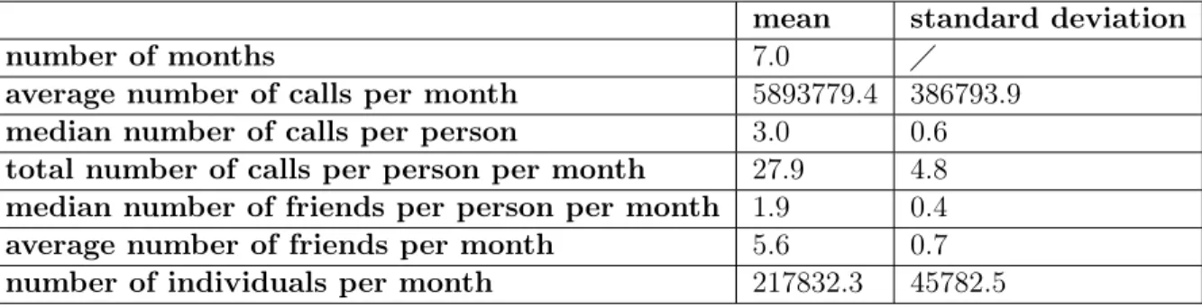
Table 2.1: Basic statistics about the mobile phone data set in country A.

mean standard deviation

number of months 7.0 

average number of calls per month 5893779.4 386793.9

median number of calls per person 3.0 0.6

total number of calls per person per month 27.9 4.8

median number of friends per person per month 1.9 0.4

average number of friends per month 5.6 0.7

number of individuals per month 217832.3 45782.5

Table 2.2: Basic statistics about the mobile phone data set in the city in country B.

mean standard deviation

number of months 12.0 

average number of calls per month 7634397.4 1089728.8

median number of calls per person 43.6 30.6

total number of calls per person per month 91.7 27.3

median number of friends per person per month 18.2 2.2

average number of friends per month 11.2 2.2

number of individuals per month 646163.2 37403.7

time instances of each period. In the case of country A, for each performance day we choose the observational period 𝑇 to be a period of 𝜏 = 24 hours, starting with the beginning of the performance. In the case of Merida, for each day within three months after the store was opened, we choose 𝑇 to be a period of 𝜏 = 72 hours, starting with the beginning of the day. The motivation behind a different 𝜏 for the two data sets is as follows. The cultural performance took place only on the weekdays in a given month, therefore individuals needed to decide in a reasonably short period. In comparison, the influence on the decision to visit the store may take longer to appear, both because people do not go to stores every day and because they know that the store would remain open for an extended period.

We introduce three key concepts in this section of my thesis. First, we define 𝒟𝑇

as the set of initial adopters for the observation period 𝑇 . We identify people as initial adopters if they were connected to a cell tower close to the performance venue or the store location during a time interval at the beginning of the period 𝑇 . In the case of country A, such an interval is defined as the time window of the performance

(with a buffer time of ± 30 minutes). In the case of Merida, the interval is defined as the first day in 𝑇 . Second, we construct an information cascade as a directed graph 𝒞𝑇 = (ℐ𝑇, ℰ𝑇), where ℐ𝑇 = {1, 2, 3, ..., 𝑛} is a set of 𝑛 individuals who have at

least one cell phone activity in 𝑇 , and ℰ𝑇 = {(𝑖, 𝑗)} is a collection of ordered node

pairs (𝑖, 𝑗) conditioned on that 𝑖 possesses information about the product when the communication with 𝑗 took place and that 𝑖 spreads the information to 𝑗. Next, we define a path of length 𝐾 − 1 between individual 𝑖 and 𝑗 in 𝒞𝑇 as a sequence of distinct

individuals, 𝑖1, ..., 𝑖𝑘, such that 𝑖1 = 𝑖, 𝑖𝑘 = 𝑗, and (𝑖𝑘, 𝑖𝑘+1) ∈ ℰ𝑇 for 𝑘 ∈ {1, ..., 𝐾 − 1}.

The social distance from individual 𝑖 to individual 𝑗, sd(𝑖, 𝑗), is defined as either the length of the shortest path from 𝑖 to 𝑗 in the cascade 𝒞𝑇 if such a path exists, or +∞

otherwise. This allows us to define the third concept, hop index for individual 𝑖, as the minimum length of the shortest paths from 𝑖 to all 𝑗 ∈ 𝒟𝑇:

ℎ𝑖 = min{sd(𝑖, 𝑗)| ∀𝑗 ∈ 𝒟𝑇}, for 𝑖 ∈ ℐ𝑇. (2.1)

Therefore, an individual 𝑖 of hop index ℎ is ℎ-degree of separation from the closest adopter in 𝒟𝑇. An illustration of these three concepts are shown in Figure 2-1.

For the cultural performance in country A, 19 observation periods generated 16,043 adopters in total. In both cases, we construct the information cascade for each 𝑇 , as shown in Figure 2-1 and compute the hop index for each individual in ℐ𝑇.

The adoption likelihood of each hop are shown in Figure 2-11 of section 2.7. The information cascades cover 161,857 individuals (who are in various treatment groups with different ℎ), with another 71,337 disconnected from the information cascades (who are in the control group). For the store in Merida, 123 observation periods in the three months after the store opened generated 4736 adopters in total. There are 86,413 and 106,340 individuals involved in and disconnected from the information cascades, respectively.

Figure 2-1: An illustration of initial adopters, information cascade, and the hop indexes. In the information cascade 𝒞𝑇 shown in the figure, within an

observation period 𝑇 , the initial adopter Anne (colored green) passes information to her neighbors, Bob, Eva, Cathy, and Daniel, who after receiving information from Anne continue to pass the information onwards. Labeled with hop index one, they further diffuse the information to Franklin, Greg, Helen, Isabel, Jack, and Kate, who are then on hop index two. The process continues until the end of the observation period. Among the people who receive information, Bob, Isabel, and Daniel (colored blue) decided to adopt the behavior, while others (colored grey) decided not to.

2.3.2

Matching framework

We use propensity score matching to yield the estimate of social influence by condi-tioning on individual preference revealed by mobility patterns [120, 166]. Specifically, we consider an individual-destination matrix M where the 𝑗-th row and 𝑖-th column correspond to the 𝑗-th destination (location of the 𝑗-th cell tower) and 𝑖-th individual, respectively, and M𝑗𝑖 represent the number of times that individual 𝑖 has visited

destination 𝑗 during a period prior to the observation periods (around six months in both cases). We then project M onto a subspace spanned by the top eigenvectors of its covariance matrix to obtain an eigen-preference matrix in which the 𝑖-th column, 𝑥𝑖, represents the preferences of individual 𝑖. Specifically, we choose 14 eigenvectors

for the adoption of attending the cultural performance and 44 for the adoption of visiting the retail store, such that they explain at least 80% of the variance of the covariance matrix in each case.

(a) an explorative pattern (b) an exploitative pattern

Figure 2-2: Two types of mobility frequency patterns during weekends, re-vealing different individual preferences: (a) an explorative pattern; (b) an exploitative pattern. The intensity of the color represents the normalized visitation frequency, i.e., the darker red color corresponds to a more frequent visit.

mobility frequency patterns in Figure 2-2, where the color intensity represents the normalized visitation frequency. Figure 2-2(a) describes the mobility history of an individual with diverse activity patterns, i.e., a person who explores various parts of the country during the weekends (explorative pattern), while Figure 2-2(b) describes the mobility history of an individual who spends most of her weekends in crowded shopping districts (exploitative pattern).

For the information cascade 𝒞𝑇 constructed for each observation period 𝑇 , we

define a treatment group in hop ℎ as the group of individuals with a finite hop index ℎ (and thus of social distance ℎ from the closest adopters in 𝒟𝑇) and a control group

in which individuals have an infinite hop index (and thus are not connected to any adopter in 𝒟𝑇). In each period, 𝑇 , then, there are multiple treatment groups, one for

each finite hop index. For each treatment group, every individual is then matched to one in the control group using propensity score matching [120, 166], where the propensity score of being treated in hop ℎ is defined as the conditional probability of being connected to the initial adoption via ℎ hops that is estimated using individuals’ preferences via logistic regression. The propensity score matching operates under the conditional unconfoundedness assumption, the adoption behaviors are independent of

the exposure, and that all individuals have a positive conditional probability of being exposed to the information or otherwise. Therefore conditional unconfoundedness implies that exposure to social influence is also unconfounded conditional on propensity score [120, 166].

Under the proposed matching framework, the difference in adoption rate between each treatment group and the control group is the difference in adoption likelihood due to social influence for that particular treatment. For example, the difference in the adoption likelihood for the treatment group in hop ℎ, Δ𝐴ℎ, is computed as,

Δ𝐴ℎ = 1 |Ψ| ∑︁ 𝑇 ∈Ψ 1 |ℳ𝑇| |ℳ𝑇| ∑︁ 𝑚=1 (𝑧_𝑚ℎ − 𝑧𝑐 𝑚), (2.2)

where 𝑧_𝑚ℎ and 𝑧_𝑚𝑐 are the adoption decisions of the individuals in the 𝑚-th matched pair from the treatment group on ℎ and the control group, respectively, |ℳ𝑇| is the

cardinality of the set ℳ𝑇 that contains all matched pairs in period 𝑇 , and |Ψ| is

the total number of observation periods. The adoption rate of the control group is denoted as 𝐴0. The difference in the adoption likelihood between the two groups

due to social influence thus establishes an upper bound2 _{of the extent to which social}

influence, rather than homophily, explains the adoption behavior [14].

2.4

Long range of social influence

We apply the behavioral matching framework mentioned section 2.3 to estimate the treatment effect of social influence on the likelihood of adoption for the two behaviors under consideration. In Figure 2-3 (a) and (b), the purple dashed line shows the the difference in the adoption likelihood of the treatment group and the control group due to social influence (y-axis) concerning different hop indexes (x-axis). For both

2_{This is mainly due to the difficulty in controlling for unobserved confounding variables using}

matching-based methods in observational studies. For country A, to partly address the issue that tourists may travel together, we remove individual pairs who are potentially on the same trip to country A. This can be inferred based on whether individuals have stayed at the same hotel on the same nights. For country B, however, it is difficult to verify whether people have received advertisements about the new store via mails, TV, or online sources.

attending a performance and visiting a store, social influence increases the likelihood of future adoption. The effect of social influence is particularly strong for individuals who had direct phone communication with the past adopters, with an increase of 148% (attending a performance) and 169% (visiting a store) in the likelihood of future adoption. To study whether behavioral patterns omit some information contained in socio-demographics, we compare the matching estimates with merely behavioral covariates, as well as supplementing that with socio-demographics in the case of visiting the retail store. By comparing the point estimates and confidence intervals in Figure 2-4, we see that the estimates by matching with and without socio-demographic are almost the same except for a slight difference in the first hop, which indicates that socio-demographics provide a subset of information embedded in behavioral covariates.

More interestingly, we observe the long range effect of social influence over the communication network, originating from the initial adopters’ direct contacts and expanding over longer social distances in the information cascades. Specifically, the difference in adoption likelihood of the treatment group and the control group due to social influence shows a decaying pattern from hop one onwards but persists up to more than three degrees of separation in both cases. This rather surprising result suggests that initial adopters’ communication may have a hidden impact on the decision-making of individuals far beyond the immediate contact circle. The comparison between the the difference in adoption likelihood for the treatment and the control group in the two cases also seems to imply a difference in virality between the two adoption behaviors.

We perform some robustness checks on the empirical results. First, to mimic the random assignment of treatment in a controlled experiment, we need to ensure that individual pairs in the treatment and the control groups are sufficiently similar. we first evaluate whether there is sufficient overlap between the individual pairs in the treatment and the control group. In other words, the covariates – the preference vectors 𝑥𝑗 in our case – must be balanced between the matched pairs to remove the

confounding effects. To this end, we use the standardized mean difference (SMD) to evaluate whether the covariates in the treatment and control groups demonstrate sufficient overlap [68]. The SMD is calculated as the difference in means in the unit of

1 2 3 4 5 6 hop index 0 50 100 150 200 250 300 Ah A0 % PSM random matching shuffling test

(a) attending cultural performance

1 2 3 4 5 6 hop index 0 50 100 150 200 250 300 Ah A0 % PSM random matching shuffling test

(b) visiting retail store

Figure 2-3: Percentage improvement in adoption rate relative to the control group due to social influence via phone communication network (Δ𝐴ℎ): (a)

attending cultural performance; (b) visiting the retail store. The y-axis is the difference in adoption likelihood of the two groups, and the x-axis is the hop index. The purple, blue, and red dashed lines show the estimated effect of social influence using PSM, random matching, and PSM after a shuffling test, respectively. The shaded regions correspond to the 5% and 95% confidence intervals from bootstrap sampling. The higher and lower end of the vertical line indicates the 5% and 95% interval.

pooled standard deviation as follows:

SMD = _√︁𝑥𝑗,ℎ− 𝑥𝑗,𝑐 (𝜎2

𝑗,ℎ+ 𝜎𝑗,𝑐2 )/2

, (2.3)

where 𝑥𝑗,ℎ and 𝑥𝑗,𝑐 are the means of the covariates 𝑥𝑗 for the treatment group on hop

ℎ and the control group, respectively, and 𝜎𝑖,ℎ and 𝜎𝑖,𝑐 are the standard deviations of

covariates 𝑥𝑗 for the treatment group on hop ℎ and the control group, respectively. As

a rule of thumb, SMD of less than 0.1 for a particular variable demonstrates sufficient overlap between the treatment and control groups for that variable. All the variables we choose in Figure 2-5 and 2-6 pass this robustness check.

Second, we show as the blue dashed line in Figure 2-3 the estimated influence without controlling for homophily where, instead of the PSM strategy, a member of the treatment group is randomly matched to another in the control group. In both cases, we observe an overestimation of the effect of social influence by about 100% with random matching, which is consistent with the finding in a previous study on the adoption of an online application [14]. To further validate results on the effect of

1 2 3 4 5 6 hop index 0 50 100 150 200 250 300 Ah A0

%

Figure 2-4: Matching on behavioral covariates, and on both behavioral co-variates and socio-demographics, for the adoption behavior of visiting the retail store. The y-axis is the difference in adoption likelihood of the two groups, and the x-axis is the hop index. The bar plot and the vertical lines correspond to the mean, 5%, and 95% confidence intervals, respectively. The blue and red bars correspond to behavioral matching, and behavioral + socio-demographics matching.

social influence, we test the "random shuffling" strategy proposed by [9] to exclude the effect of homophily or unobserved confounding variables that may induce statistical correlation between the actions of friends and therefore generate the observed decaying patterns. To this end, we randomly assign individuals to the control and treatment groups, with a randomized hop index for individuals assigned to the latter. We then compute the difference in the adoption likelihood due to social influence using the PSM strategy, and the results are shown as the red dashed line in Figure 2-3. Both the increased likelihood of adoption and the decaying patterns mostly disappear, which verifies that the observed patterns are not likely to be driven merely by the effect of homophily or unobserved confounding variables.

Finally, we also use a post-Lasso estimation method to estimate the coefficients for treatments with a data-driven penalty [33]. We use post-Lasso logistic regression to estimate the difference in adoption likelihood of the two groups, which applies ordinary least squares to the model selected by Lasso [32, 33]. The results are shown in Figure 2-7. The estimates via the post-lasso logistic regression, as shown in the blue bar plots, also display a long range effect of social influence and penetrates deep into the communication network, which demonstrates the robustness of our results.

Figure 2-5: SMD for the matching between the control group and the dif-ferent treatment groups (difdif-ferent hop indexes ℎ), in the case of attending cultural performance.

Figure 2-6: SMD for the matching between the control group and the dif-ferent treatment groups (difdif-ferent hop indexes ℎ), in the case of visiting retail store.