HAL Id: hal-02008499
https://hal.inria.fr/hal-02008499
Submitted on 8 Mar 2021
HAL is a multi-disciplinary open access archive for the deposit and dissemination of sci-entific research documents, whether they are pub-lished or not. The documents may come from teaching and research institutions in France or abroad, or from public or private research centers.
L’archive ouverte pluridisciplinaire HAL, est destinée au dépôt et à la diffusion de documents scientifiques de niveau recherche, publiés ou non, émanant des établissements d’enseignement et de recherche français ou étrangers, des laboratoires publics ou privés.
information: Comparative evaluation of methods by
simulation and application to real data
Bernard Silenou, Marta Avalos, Catherine Helmer, Claudine Berr, Antoine
Pariente, Hélène Jacqmin-Gadda
To cite this version:
Bernard Silenou, Marta Avalos, Catherine Helmer, Claudine Berr, Antoine Pariente, et al.. Health administrative data enrichment using cohort information: Comparative evaluation of methods by sim-ulation and application to real data. PLoS ONE, Public Library of Science, 2019, 14 (1), pp.e0211118. �10.1371/journal.pone.0211118�. �hal-02008499�
Health administrative data enrichment using
cohort information: Comparative evaluation
of methods by simulation and application to
real data
Bernard C. Silenou1, Marta AvalosID1,2, Catherine Helmer1, Claudine Berr3, Antoine Pariente1,4, Helene Jacqmin-Gadda1
*
1 Univ. Bordeaux, INSERM, ISPED, Bordeaux Population Health Center, Bordeaux, France, 2 Inria SISTM
Team, Talence, France, 3 Univ. Montpellier, INSERM, Montpellier Cedex, France, 4 CHU de Bordeaux, Pole de Sante´ Publique, Service de Pharmacologie Me´dicale, Bordeaux, France
Abstract
Background
Studies using health administrative databases (HAD) may lead to biased results since infor-mation on potential confounders is often missing. Methods that integrate confounder data from cohort studies, such as multivariate imputation by chained equations (MICE) and two-stage calibration (TSC), aim to reduce confounding bias. We provide new insights into their behavior under different deviations from representativeness of the cohort.
Methods
We conducted an extensive simulation study to assess the performance of these two methods under different deviations from representativeness of the cohort. We illustrate these approaches by studying the association between benzodiazepine use and frac-tures in the elderly using the general sample of French health insurance beneficiaries (EGB) as main database and two French cohorts (Paquid and 3C) as validation samples.
Results
When the cohort was representative from the same population as the HAD, the two methods are unbiased. TSC was more efficient and faster but its variance could be slightly underesti-mated when confounders were non-Gaussian. If the cohort was a subsample of the HAD (internal validation) with the probability of the subject being included in the cohort depending on both exposure and outcome, MICE was unbiased while TSC was biased. The two meth-ods appeared biased when the inclusion probability in the cohort depended on unobserved confounders. a1111111111 a1111111111 a1111111111 a1111111111 a1111111111 OPEN ACCESS
Citation: Silenou BC, Avalos M, Helmer C, Berr C, Pariente A, Jacqmin-Gadda H (2019) Health administrative data enrichment using cohort information: Comparative evaluation of methods by simulation and application to real data. PLoS ONE 14(1): e0211118.https://doi.org/10.1371/journal. pone.0211118
Editor: Philipp D. Koellinger, Vrije Universiteit Amsterdam, NETHERLANDS
Received: May 28, 2018 Accepted: January 8, 2019 Published: January 31, 2019
Copyright:© 2019 Silenou et al. This is an open access article distributed under the terms of the
Creative Commons Attribution License, which permits unrestricted use, distribution, and reproduction in any medium, provided the original author and source are credited.
Data Availability Statement: To request access to EGB data, please contact The National Institute for Health Data (Institut National des Donne´es de Sante´, INDS) (website:http://www.indsante.fr/). The authors cannot share the data from EGB underlying this study because publicly sharing EGB data is forbidden by law according to The French national data protection agency (Commission Nationale de l’Informatique et des LIberte´s, CNIL); regulatory decisions AT/CPZ/SVT/JB/DP/ CR05222O of June 14, 2005 and DP/CR071761 of
Conclusion
When choosing the most appropriate method, epidemiologists should consider the origin of the cohort (internal or external validation) as well as the (anticipated or observed) selection biases of the validation sample.
Introduction
Health administrative databases (HAD) are a valuable source of data for studying the associa-tion between treatment and disease outcome [1–4]. In France, the national inter-regime infor-mation system on health insurance (SNIIRAM) database covers the entire French population (65 million inhabitants) [2–4]. This database includes demographic (age, gender, city of resi-dence) and out-hospital reimbursement (drug dispensing and long-term diseases). A 1/97th random permanent sample of SNIIRAM, the general sample of French health insurance bene-ficiaries (Echantillon Ge´ne´raliste des Be´ne´ficiaires, EGB), which is representative of the national population of health insurance beneficiaries, was composed in 2005 to allow a 20-year follow-up. These administrative databases are readily available for epidemiological research. The large number of patients without loss of follow-up allows for sufficient powering of stud-ies. Furthermore, the information is plentiful, comprehensive and detailed, without any exclu-sions [2–4].
Administrative databases are not without limitations. Information on potential confound-ers is often missing and recent reviews have described current strategies to control for unmea-sured confounding in HAD [5–7]. Sensitivity analyses [8–10] have been helpful in the past to adjust for bias due to unmeasured confounders, but they are limited because they cannot con-trol for multiple unmeasured confounding variables. Occasionally, detailed confounding information missing from the HAD (main sample) can be procured from a validation sample that may be a subsample of the HAD (internal validation sample) or another cohort assumed to be representative of the same population (external validation sample). Methods have been developed to incorporate information from the validation sample in the analysis of HAD to reduce confounding bias. Three of these methods are based on the propensity score [11]. Two-stage calibration (TSC) [12] and propensity score calibration (PSC) [13] aim to adjust for the propensity score instead of individual confounders and consider the propensity score com-puted only with the observed confounders (crude propensity score) as a measure with error of the propensity score including all the confounders (precise propensity score). McCandless and colleagues [14] summarized unobserved confounders in a summary score built using the pro-pensity score methodology and proposed a Bayesian approach (BayesPS) to adjust for this missing score. Multivariate imputation by chained equations (MICE) seeks to adjust directly for the unobserved confounders [15]. MICE has proved to be an effective technique in control-ling bias due to unmeasured confounding [16–18]. Unlike the other methods, PSC does not need the outcome variable to be measured in the validation data but relies on the additional surrogacy assumption that measurement error is independent of the outcome variable, given the precise propensity score and exposure [13]. BayesPS does not need the surrogacy assump-tion but requires either the assumpassump-tion that the observed confounders are independent of the unobserved ones or a Gaussian linear model for the summary score given the observed con-founders; this may be unrealistic for few categorical unmeasured confounders. Simulation studies have shown that PSC is more biased and generally has larger variance than the other three methods, while the performance of BayesPS is similar to that of MICE [12,14]. Several August 28, 2007. Moreover, in the interest of
participant confidentiality and in keeping with data sharing guidelines imposed by the National Commission on Informatics and Liberty (CNIL), the data from 3C and Paquid cohorts used in this study are available upon request. Interested researchers may [email protected]
for access to 3C data and the principal investigator of the Paquid cohort Pr Jean-Franc¸ois Dartigues ([email protected]) or Dr Catherine Helmer (Catherine.Helmer@u-bordeaux. fr) for access to Paquid.
Funding: The present study is part of the Drugs Systematized Assessment in real-liFe Environment (DRUGS-SAFE) research program funded by the French Medicines Agency (Agence Nationale de Se´curite´ du Medicament et des Produits de Sante´, ANSM). This program aims at providing an integrated system allowing the concomitant monitoring of drug use and safety in France. The potential impact of drugs, frailty of populations and seriousness of risks drive the research program. This publication represents the views of the authors and does not necessarily represent the opinion of the French Medicines Agency. The Paquid study was funded by Ipsen and Novartis and the Caisse Nationale de Solidarite´ et d’Autonomie. The Three-City study was supported by Sanofi-Aventis, the Fondation pour la Recherche Me´dicale, the Caisse Nationale Maladie des Travailleurs Salarie´s, Direction Ge´ne´rale de la Sante´, MGEN, Institut de la Longe´vite´, and Conseils Re´gionaux d’Aquitaine and Bourgogne, Fondation de France, Ministry of Research-INSERM Programme “Cohortes et collections de donne´es biologiques”, Agence Nationale de la Recherche ANR PNRA 2006 and LongVie 2007, and the "Fondation Plan Alzheimer" (FCS 2009-2012). The funders had no role in study design, data collection and analysis, decision to publish, or preparation of the manuscript.
Competing interests: The authors have declared that no competing interests exist.
studies have demonstrated the utility of these methods in real applications [8,19–21] but have highlighted the need for additional research on method diagnostics in practical situations to decide which method to use.
The objective of the present study was to compare through simulations the performance of these methods whose required assumptions are more compatible with our target application: large-scale population-based observational HAD and validation cohorts with measures of the outcome variable. Bias and robustness of MICE and TSC were assessed (1) when the validation sample was representative of the same population as the HAD and under different departures from representativeness of (2) the external and (3) the internal validation samples. Our param-eter of interest was the log-odds ratio (log(OR)) for the effect of exposure conditional on all the confounders (observed and unobserved).
To illustrate the advantages and limitations of these methods to account for unobserved confounders in HAD, MICE and TSC were then applied to the general sample of EGB to study the relationship between benzodiazepine (BZD) use and fractures in the elderly using two dif-ferent cohorts, Paquid and Three-City (3C), as validation samples [22–24].
Materials and methods
Study population
Main sample. The main database was EGB [2]. The data consisted of 60,243 subjects of at least 69 years of age in 2006 who were alive and had not dropped out of the EGB before 2009. BZD users were defined as subjects who had at least one reimbursement for BZD between October 1 and December 31, 2006. We identified 15,638 BZD users while the remaining 44,605 were considered as unexposed. The outcome of interest was fractures of all types arising in the three years following the measure of exposure, that is, between January 1, 2007 and December 31, 2009. Using information on hospital diagnoses, we found 3,260 subjects with at least one fracture. The observed potential confounders were age, gender, exposure to antihy-pertensive and non-BZD psychotropic medications.
Validation samples. The Paquid project, initiated in 1988, was designed to study the risk factors of age-related health conditions [23]. The cohort includes 3,777 subjects of at least 65 years old, from two French departments. Subjects randomly selected from the electoral rolls who agreed to participate were interviewed at their homes by trained neuropsychologists at baseline and subsequently every two or three years. At each visit, information on fractures since the last visit and drugs used at the time of the visit was collected. The validation sample consisted of 1,342 subjects visited in the 5th (T5, in 1993–94) and 8th (T8, in 1996–97) follow-up years with complete data regarding drugs used and confounding factors at T5 and fractures at T8. This ensured that the validation sample was as close as possible to the EGB sample while optimizing the sample size. At T5, information on potential confounders available in EGB (age, gender, antihypertensive and non-BZD psychotropic drugs used) was collected as well as information on potential confounders missing from EGB: body mass index (BMI), educational level (primary school diploma denoted high education versus no diploma or no education denoted low education) and depressive symptomatology measured by the Center for Epidemi-ologic Studies Depression Scale (CESD) as a binary covariate (subjects were considered as depressed if they obtained a score of more than 17 for males and 23 for females out of 60 on the CESD scale).
The 3C study is a population-based longitudinal study of the relation between vascular dis-eases and dementia including 9,294 participants aged 65 years and older at baseline in 1999 and living in three French cities (Bordeaux, Dijon and Montpellier) [24]. The validation sam-ple for this analysis consisted of 2,231 subjects from Bordeaux and Montpellier visited in the
4th (T4 in 2003–04) and 7th (T7 in 2006–07) years of follow-up. Exposure to medications and confounders were collected at T4 and fractures at T7, as in Paquid.
Ethics statement
INSERM, as a health research institute, has been authorized to use the EGB database by the French data protection authority (Commission Nationale de l’Informatique et des Liberte´s, CNIL), provided that the researcher follows specific training with certification, as the first and fifth authors (Bernard Silenou, Antoine Pariente) have obtained.
The Ethics Committee of Kremlin-Bicêtre University Hospital and Bordeaux University Hospital respectively approved study protocols for the 3C and Paquid cohorts, and each partic-ipant signed a written informed consent. All data were fully anonymized.
Adjustment methods for unobserved confounders
LetY be the binary outcome and X the binary exposure variable. Let C be the vector of
con-founders measured in both the main and the validation data andU the vector of confounders
measured only in the validation data.
Two-stage calibration. The crude propensity score is defined as the probability of being exposed given observed confoundersC (PSC= P(X = 1|C)) and the precise propensity score as
the probability of being exposed given confoundersC and U (PSP= P(X = 1|C,U)) [13,25].PSC
andPSPare estimated by logistic regression in the pooled (main+validation) and validation
data, respectively.
Lin and Chen [12] defined two models for the outcome adjusting either forPSCorPSP
logit½PðY ¼ 1jX; CÞ� ¼ d þ gX þ yf ðPSCÞ ð1Þ
logit½PðY ¼ 1jX; C; UÞ� ¼ a þ bX þ φgðPSPÞ ð2Þ
wheref and g are identity or suitable transformation functions, e.g. spline functions. TSC aims
to estimateβ in the pooled sample (�b) from ^b and ^g estimated in the validation sample, and �g estimated in the pooled sample using [12]
�
b ¼ ^b l n ð^g �gÞ andvar �b�¼var ^b
� �
l2
nwhereλ is the covariance between ^b and ð^g �gÞ andν is the
vari-ance of ð^g �gÞ;λ and ν are estimated by the sandwich estimator as detailed in the web appen-dix of [12]. Like PSC and BayesPS, TSC requires that the propensity score models are well specified and that the validation sample is representative of the main sample. More precisely, ^g and �g are assumed to be unbiased estimates ofγ and ^b is assumed to be an unbiased estimate ofβ. We will see later that departures from representativeness that do not invalidate the above assumptions are permitted (for instance, different marginal distributions of either C, X or Y). On the other hand, TSC does not need assumption regarding the relationship betweenPSC
andPSP.
Multiple imputation. Unobserved confounders in the main sample can be considered as missing data in the pooled sample, and multiple imputation such as MICE may be used to adjust for these unobserved confounders [15]. However, in this context where the proportion of missing observations forU is vast, it is recommended to increase the number of imputations
[26]. The multiple imputation approach requires the missing-at-random assumption, i.e. that the observation probability for U, which is the probability of belonging to the validation cohort
in this context, does not depend on U. Moreover, parametric assumptions are needed for imputation models. We used logistic regression as an imputation model for binary variables and predictive mean matching, which is a robust method for non-Gaussian variables, for quantitative variables [27]. All variables were included in each imputation model to preserve the correlation structure in the data.
Simulation study
We compared the performances of the methods when the external validation sample is repre-sentative of the same population as the main sample and under different departures from rep-resentativeness. The validation data were considered to be representative when the
multivariate distribution of all the variables (Y, X, C, U) in the validation sample is identical to
that of the main sample. We considered two observed (C = (C1, C2)) and two unobserved (U =
(U1, U2)) confounders. The binary exposure (X) and the binary outcome (Y) were generated
using the following logistic models:
logitðPðX ¼ 1jC; UÞÞ ¼ l0þ l1C1þ l2C2þ l3U1þ l4U2 ð3Þ
logitðPðY ¼ 1jX; C; UÞÞ ¼ b0þ bX þ b1C1þ b2C2þ b3U1þ b4U2 ð4Þ
All the data were generated under the assumption of no exposure effect (β = 0), thus avoid-ing the issue of non-collapsibility of the OR [28]. Thus, a difference in parameter estimates of
β with or without conditioning on unmeasured confounders U1andU2would solely be due to
the confounding bias of these unmeasured confounders.
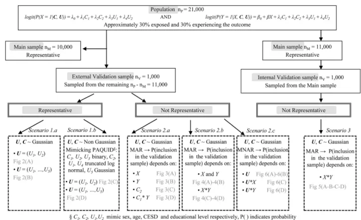
The simulation proceeded by generating a population of nP= 21,000 subjects. In scenarios
1 and 2, we focused on external validation samples, while in scenario 3, we generated an inter-nal validation sample. For scenarios 1 and 2, a representative main sample (nM= 10,000) was
randomly drawn from the population while the validation sample (nV= 1,000) was extracted
from the remaining 11,000 subjects. In scenario 1 the validation sample was representative of the population, while in scenario 2 it was not. The variableU in the main data was considered
as missing. For scenario 1, two series of simulations were run by varying the distribution of the confounders:
Scenario 1.a: Confounders U and C were generated from a standard normal distribution. Scenario 1.b: Confounders U and C were generated from non-Gaussian distributions
roughly mimicking the distributions of the sex (C1), age (C2), CESD (U1) and education (U2)
variables in the Paquid cohort.C1andU2were binary whileC2andU1followed truncated log
normal distributions. Additional simulations were performed with five unobserved confound-ers for scenarios 1.a and 1.b (for 1.b U3was binary, U4was truncated log-normal and U5was
Gaussian).
Scenario 2: The population was generated as in scenario 1.a and non-representative
valida-tion samples were selected to investigate the sensitivity of each method to various selecvalida-tion biases. The probability of inclusion in the validation sample was a function of eitherX, Y, C or C�Y (in Scenario 2.a), where�represents an interaction effect between two variables,X + Y orX�Y (in Scenario 2.b), or U, U�X or U�Y (in Scenario 2.c). Scenarios 2.a and 2.b
corre-spond to missing-at-random mechanisms, hence MICE is expected to be robust, while for sce-nario 2.c, data are missing not at random and MICE is expected to fail. TSC requires that the association betweenY and X given C alone and given C and U be identical in the validation
and the main sample. This assumption was violated in scenarios 2.b and 2.c.
Scenario 3: We performed an additional set of simulations with a non-representative
Fig 1shows the flowchart of the data generation procedure by scenario. For each scenario, we generated 500 data sets. Parameter values for data generation are specified inS1 File. We compared estimates of the log(OR) for the exposure X obtained from MICE with 10 imputa-tions, TSC with either identity function (TSC) or natural cubic spline using 2 knots (TSC_SP) forf and g in models (1) and (2), logistic regression on the main data adjusting for (U,C)
(UC_MAIN) or forC only (C_MAIN), on the pooled data adjusting for (U,C) (UC_POOL) or
forC only (C_POOL) and on the validation data adjusting for (U,C) (UC_VAL).
The bias (with respect to the target parameterβ = 0) was computed as the mean of the estimates�^b over the 500 replicates. The efficiency of the various estimates was compared through the cross-replications standard error (empirical standard error,ESEð^bÞ). For each data set (k = 1,. . .,500), the 95% confidence interval of the estimate was computed as ^bk� 1:96ASEð^bkÞ whereASEð^bkÞ is the estimated asymptotic standard error of the considered estimate on sample k. The coverage rate of the confidence interval was computed as the pro-portion of times this CI included the true value 0 over the 500 replicates. A coverage rate will be close to the nominal value of 95% means if (i) the bias for the parameter estimate ^b is negli-gible compared to its variance and (ii) the variance of ^b is correctly estimated. With 500 repli-cates, the coverage rate is significantly different from 95.0 when it is outside 93.1–96.9. Finally the mean square error (MSE) was computed asMSE ¼P500k¼1ðb b^kÞ
2
=500; the MSE allows a
global comparison of the estimators since it is the sum of their square bias and their variance. Analyses were performed with R version 3.2.3.
Fig 1. Flowchart of the data generation procedure by scenario for internal and external validation samples. MAR and MNAR correspond to missing-at-random and missing-not-at-random mechanisms, respectively.
Results
Simulation
Figs2–6summarize the main simulation results through the mean estimates± ESE and the coverage rates of the 95% confidence interval based on the asymptotic standard error esti-mated on each data set.S1–S5Tables display detailed simulation results including mean asymptotic standard error, empirical standard error, mean square error and mean computa-tion time.
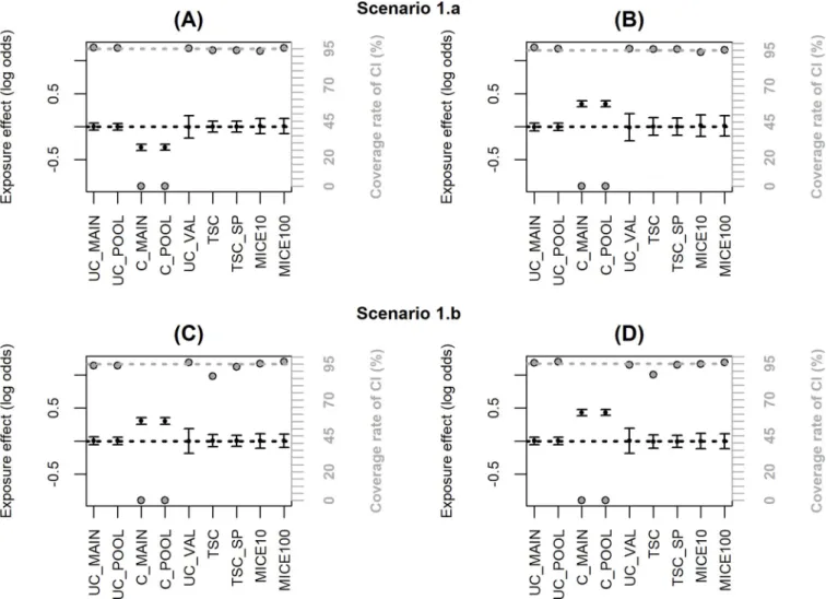
Fig 2andS1 Tabledisplay the results for the estimates of the effect of exposure when the validation data are representative of the same population as the main sample (scenario 1). The estimate adjusted only forC from the main sample (C_MAIN) highlights the bias due to the
unmeasured confounders. The adjusted estimate from the validation sample (UC_VAL) is unbiased but has a larger standard error owing to the small sample size. All the correction methods are unbiased with a coverage rate of the CI close to 95%, and the two TSC estimators appear to be the most efficient since their ESE are the smallest. This is confirmed by comparing
Fig 2. Simulation results with a representative external validation sample (scenario 1); coverage rate of 95% confidence interval (grey dot with black margin) and mean estimated log-odds ratio for the exposure effect (black dot)± empirical standard error: (A) two unobserved Gaussian confounders, (B) five unobserved Gaussian confounders, (C) two unobserved non-Gaussian confounders, (D) five unobserved non-Gaussian confounders. The grey dotted line corresponds to the nominal value of the coverage rate of the 95% confidence interval. The black dotted line is the true value ofβ (0).
the MSE which is the sum of the bias and variance: TSC and TSC_SP have the smallest MSE in S1 Table. However,Fig 2C and 2Dshow a slight under-coverage of the CI for TSC when the confounders are non-Gaussian (86.6% and 87.4% instead of 95%). This is explained by the slight underestimation of the standard error (ASE compared to ESE in case 1.b inS1 Table) because the variance of estimated parameters from the propensity score model is neglected [29]. By using the true parameter value for the propensity score model instead of the estimates obtained on the validation sample, this underestimation disappears (results not shown). When additional spline parameters are estimated in TSC_SP, the impact of the variance of the pro-pensity score model is negligible and the coverage rate of the CI remains correct. In scenario 1, we also compared MICE using either 10 or 100 imputations. Results inS1 Tableshow negligi-ble differences between 10 and 100 imputations in term of bias and efficiency but a 10-fold increase in computation time. For the other scenarios, MICE was thus computed using 10 imputations only. The TSC approaches requires the least computation time: less than 0.1sec-onds per sample for 5 unobserved confounders versus 30 or 40 sec0.1sec-onds for MICE with 10 imputations depending on the imputation methods (predictive mean matching takes more time than logistic regression).
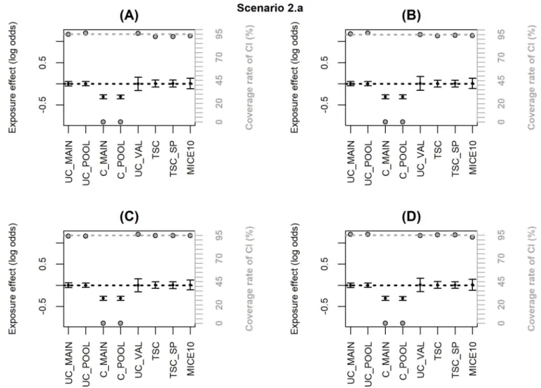
Fig 3. Simulation results when the inclusion probability in the external validation sample (notated P) depends only onX, Y, C or C�Y (scenario 2.a);
coverage rate of 95% confidence interval (grey dot with black margin) and mean estimated log-odds ratio for the exposure effect (black dot)± empirical standard error: (A) logit(P) =−2.7+log(4)X, (B) logit(P) = −2.7+log(4)Y, (C) logit(P) = −2.7+log(4)C2, (D) logit(P) =−2.5+log(2)C1+log(2)Y+log(4)C1�Y. The grey dotted line corresponds to the nominal value of the coverage rate of the 95% confidence interval. The black dotted line is the true value ofβ (0).
When the inclusion probability in the validation sample depends only onX, Y, C or C�Y, the associations betweenX and Y given C alone and given C and U are identical in the main
and the validation samples and U is missing at random. Thus, both TSC and MICE remain unbiased with a coverage rate close to the nominal value (scenario 2.a,Fig 3,S2 Table).
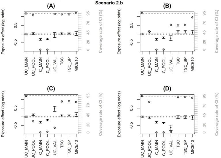
When the inclusion probability in the external validation sample depends onX and Y, TSC
and MICE lead to significant bias (scenario 2.b,Fig 4andS3 Table). When the dependence on
X and Y is moderate (OR = 2,Fig 4A), the bias has negligible impact on the coverage rate of the 95% CI; but the bias increases with the strength of the dependence (OR = 4,Fig 4B) and more dramatically when the inclusion probability depends on an interactionX�Y (Fig 4C and 4D) leading to a major undercoverage of the CI. These bad results were expected for TSC since the selection makes the association betweenY and X different between the validation and the
main sample (as shown by the bias in UC_VAL). However, bias in MICE estimates may appear surprising because the missing data are at random (MAR). To explain this result, we must emphasize that the objective of the correction methods is to estimate the adjusted association betweenX and Y in the population of which the pooled sample is representative. When a
non-Fig 4. Simulation results when the inclusion probability in the external validation sample (notated P) depends onX + Y or X�Y (scenario 2.b); coverage
rate of 95% confidence interval (grey dot with black margin) and mean estimated log-odds ratio for the exposure effect (black dot)± empirical standard error: (A) logit(P) = -2.6+log(2)X+log(2)Y, (B) logit(P) = -3.2+log(4)X+log(4)Y, (C) logit(P) = -2.7+log(2)X+log(2)Y+log(2)X�Y, (D) logit(P) = -2.5+log(2)X
+log(2)Y-log(2)X�Y. The grey dotted line corresponds to the nominal value of the coverage rate of the 95% confidence interval. The black dotted line is the true
value ofβ (0).
representative external validation sample is used, the pooled and main samples do not reflect the same population and the association betweenX and Y may be different in the two
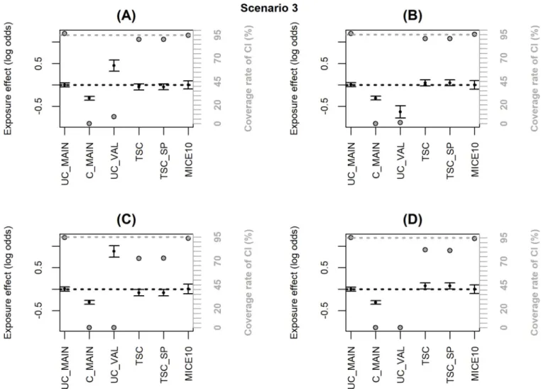
popula-tions. Indeed, inFig 4andS3 Table, UC_MAIN and UC_POOL are different and we can see that MICE estimate is close to UC_POOL. On the other hand, when an internal validation sample is used (i.e. the validation sample is a subsample of the main HAD), the pooled and main samples are identical even if the validation sample is not representative. In scenario 3, we generated a non-representative internal validation sample where the inclusion probability depended onX�Y and we checked that MICE was unbiased with nominal coverage rate while TSC was still biased (Fig 5andS4 Table).
Finally, all the correction methods fail when the inclusion probability in the validation sam-ple depends onU (scenario 2.c,Fig 6,S5 Table), and especially when it depends onX�U or
Y�U (Fig 6C and 6D). The imputation method fails because the confounders are not missing at random, while TSC fails because the confounding effect ofU is different in the validation and Fig 5. Simulation results with a non-representative internal validation sample where the inclusion probability (notated P) depended onX�Y (scenario
3); coverage rate of 95% confidence interval (grey dot with black margin) and estimated log-odds ratio for the exposure effect (black dot)± empirical standard error: (A) logit(P) =−2.7+log2X+log2Y+log2X�Y, (B) logit(P) =−2.5+log2X+log2Y−log2X�Y, (C) logit(P) =−2.8+log2X+log2Y+log4X�Y, (D) logit
(P) =−2.4+log2X+log2Y−log4X�Y. The grey dotted line corresponds to the nominal value of the coverage rate of the 95% confidence interval. The black dotted
line is the true value ofβ (0).
the main sample. Note however that, adjusting onU, the parameter estimate in the validation
sample is unbiased (UC_VAL) with this scenario (thus UC_POOL is also unbiased).
Application
Table 1presents the distribution of all the variables in the main and validation samples. BZD users tended to be less educated and more depressed, suggesting that these factors could be confounders. We observed some differences in the distributions of BZD users (X), fractures (Y) and educational levels (U) between the three samples.
MICE and TSC were applied to estimate the log(OR) of the association between exposure to BZD and fractures adjusted for the observed confoundersC (age, gender, anti-hypertensive
and non-BZD psychotropic) and unobserved confoundersU (BMI, CESD and education). As
a comparison, we also estimated the log(OR) adjusted forC in EGB (C_MAIN) and for (U, C)
in the validation sample (UC_VAL). Results are displayed inTable 2. Without adjusting forU
in EGB, BZD users had a higher risk of fractures (log(OR) = 0.36, 95% CI: 0.28, 0.44). By adjusting for BMI, education and CESD in the Paquid cohort, the regression parameter
Fig 6. Simulation results when the inclusion probability in the external validation sample (notated P) depends onU1; coverage rate of 95% confidence
interval (grey dot with black margin) and mean estimated log-odds ratio for the exposure effect (black dot)± empirical standard error: (A) logit(P) = -2.2 +log(2)U1, (B) logit(P) = -2.7+log(4)U1, (C) logit(P) = -2.3+log(2)U1+log(2)X�U1, (D) logit(P) = -2.5+log(2)U1+log(2)Y�U1. The grey dotted line corresponds to the nominal value of the coverage rate of the 95% confidence interval. The black dotted line is the true value ofβ (0).
dropped by approximately half (0.17, [-0.25, 0.59]), while it was null in 3C. The three correc-tion methods using Paquid as validacorrec-tion sample highlighted an associacorrec-tion between BZD and fractures in the pooled sample, with log(OR) close to the adjusted estimate in the validation sample but with smaller variance. These results were consistent with the simulation results. On the other hand, although the estimated adjusted log(OR) was null in 3C (UC_VAL), estima-tions obtained with the correction methods were very close to the estimate adjusted only forC
in EGB.
To explain these differential results, we estimated two logistic regressions to identify factors associated with inclusion in 3C or Paquid, respectively, versus EGB. The occurrence of frac-tures and exposure to BZD were both associated with inclusion in Paquid (OR = 1.79, p<0.001 and OR = 1.31, p<0.001, respectively) but their interaction was not significant (OR = 0.83, p = 0.35). According to our simulations (Fig 4A), the bias of adjustment methods in this case should be negligible. On the other hand, the interaction between the occurrence of fractures
Table 1. Description of study population in main (EGB, n = 60,243, 2006–2009) and validation samples (Paquid, n = 1,342, 1993–1997; 3C, n = 2,231, 2003–2007) in France.
Baseline variables EGB Paquid 3C
No-BZD BZD No-BZD BZD No-BZD BZD
n (%) 44,605 (74) 15,638 (26) 907 (68) 435 (32) 1,727 (77) 504 (23) Age in y, mean (SD) 78.1 (7.2) 78.1 (6.4) 77.9 (5.7) 78.1 (5.2) 76.6 (4.8) 77.8 (5.1) Fractures % 4 8 8 11 10 12 Female % 57 73 51 77 59 75 Anti-hypertensive % 47 72 58 70 61 61 Other psychotropics % 8 32 10 29 9 29 High education % 77 68 94 90 CESD % 5 18 7 16 BMI in kg/m2, mean (SD) 25.0 (3.7) 24.4 (3.8) 25.5 (3.8) 25.3 (4.7)
Abbreviations: BMI, body mass index; BZD, exposure to benzodiazepine; CESD, Center for Epidemiologic Studies Depression Scale.
https://doi.org/10.1371/journal.pone.0211118.t001
Table 2. Estimates of exposure effect (log-odds ratio) of association between BZD and fractures; EGB database (n = 60,243, 2006–2009) and Paquid (n = 1,342, 1993–1997) and 3C (n = 2,231, 2003–2007) cohorts in France.
Methods log(OR) SE 95% CI
C_MAIN 0.36 0.04 0.28, 0.44
EGB and Paquid
UC_VAL 0.17 0.21 -0.25, 0.59 TSC 0.20 0.05 0.11, 0.29 TSC_SP 0.23 0.04 0.14, 0.31 MICE 0.25 0.07 0.12, 0.38 EGB and 3C UC_VAL 0.00 0.17 -0.33, 0.33 TSC 0.32 0.02 0.28, 0.37 TSC_SP 0.34 0.02 0.30, 0.37 MICE 0.32 0.04 0.24, 0.40
Abbreviations: CI, confidence interval; OR, odds ratio; SE, standard error. MICE was implemented with 100 imputations. TSC_SP was implemented with 5 knots.
and exposure to BZD was significant in the logistic regression for inclusion in 3C versus EGB (OR = 0.64, p = 0.007). This means that 3C sample is not representative of the EGB population with respect to the association between BZD and fractures. This sample is an urban and highly educated sample where the causes of fractures or the BZD use pattern may be different from the overall French population. This corresponds to a situation where the correction methods are highly biased (Fig 4C and 4D).
Discussion
Claims data are increasingly used for epidemiological research, but results may be biased since information on confounders is missing. A key approach to this problem is to include con-founder data from cohort studies in the same population. Strategies to control for unmeasured confounding in HAD have been the subject of recent surveys [5–7]. The surveys provide gen-eral recommendations on the choice of the strategy depending, for example, on the study design or the existence or not of a validation sample. However, to our knowledge, no study to date has provided recommendations on how to choose methods that include confounder data from cohort studies in the event of a lack of representativeness of the cohort and depending on the nature of the cohort (internal or external).
Our findings show that estimates from TSC and MICE are unbiased when the validation sample is representative of the population covered by the HAD. Multiple imputation works well in this framework despite the very high rate of missing information on confounders, even in cases where the unobserved confounders have nonstandard distributions, thanks to the robustness of imputation by predictive mean matching [27]. Nevertheless, MICE requires more computation time—an issue to consider when dealing with very large HAD—and is less efficient than TSC. When unobserved confounders have nonstandard distributions, variances may be slightly underestimated with TSC, but TSC_SP is more robust. A way to avoid this issue could be to apply TSC, adjusting directly on C and U instead of the propensity scores.
All methods are robust to non-representativeness except when the validation and main samples differ in the distribution of unobserved confounders or the distributions of both the outcome and the exposure. In the former case, which is untestable in practice, all methods are biased while in the latter, MICE provides an unbiased estimate in the pooled sample. Interest-ingly, the latter assumption can be evaluated in practice, as was illustrated in the BZD-fracture study.
We focused mainly on external validation samples because this is the most frequent situa-tion when existing cohorts are used as validasitua-tion samples. Owing to differences in time peri-ods, selection procedures and participation rates, such cohorts are not expected to be completely representative of the population targeted by the HAD. This motivated the investi-gation of the impact of departures from representativeness. However, some nationwide HAD are almost exhaustive, so existing cohorts in the country may be considered as internal tion samples if a linkage between the databases is possible. A clear advantage of internal valida-tion is that the measure of the exposure, outcome and observed confounders are common in both samples. In this context, the robustness of MICE is useful when the validation and main samples differ according to the distributions of both the outcome and exposure.
The analysis of the relationship between BZD and fractures using EGB data illustrates how these methods may be applied and, to some extent, how their validity may be evaluated in real data analyses. While this is not the best design for this study because it may suffer from a sur-vival bias, the analysis confirms that elderly users of BZD have an elevated risk of experiencing a fracture compared to unexposed subjects after controlling for confounders including BMI, education and CESD. The measures of exposure to drugs and outcome differed between the
validation and main samples. In Paquid and 3C, drug use was self-reported, but these measures can be considered reliable as the interviewer checked medication containers. They include over-the-counter drugs that are not collected in EGB, which records drug delivery from phar-macies based on prescriptions. However, antihypertensives, BZD and most non-BZD psycho-tropics cannot be bought in France without a prescription. Moreover, fractures in EGB are based on clinical diagnosis in hospitals, while fractures in the previous 3-year period were self-reported in the validation sample. Memory bias and diagnosis error are possible but probably low for a traumatic event such as a fracture.
Two important points should be made about this study. First, we compared estimates of the effect of exposure adjusting either for individual confounders or for propensity scores. How-ever, we checked both in the simulation study and in the application that the differences between these estimates were negligible (results not shown). Second, in general, OR is a non-collapsible measure [29], meaning that conditional and marginal ORs may be different even without a confounding effect. In the application, the differences between ORs adjusted forU
andC and adjusted only for C may be due to both a confounding effect and non-collapsibility.
Nevertheless, the simulations were conducted under the assumption of no exposure effect, where the OR is collapsible.
In conclusion, TSC and MICE can efficiently reduce confounding bias from unobserved confounders in large-scale studies when a validation sample with complete information on confounders is available. The origin (internal or external) of the validation sample as well as the anticipated or observed selection biases must be considered when choosing the most appropriate method. Future work could aim at improving variance estimates in TSC by accounting for the estimation of propensity score [29], or at correcting for selection bias in the validation sample through weighting approaches.
Supporting information
S1 File. Complements to simulation design. (DOCX)
S1 Table. Simulation results for scenario 1. (DOCX)
S2 Table. Simulation results for scenario 2.a. (DOCX)
S3 Table. Simulation results for scenario 2.b. (DOCX)
S4 Table. Simulation results for scenario 3. (DOCX)
S5 Table. Simulation results for scenario 2.c. (DOCX)
Author Contributions
Conceptualization: Catherine Helmer, Claudine Berr, Antoine Pariente, Helene Jacqmin-Gadda.
Funding acquisition: Catherine Helmer, Claudine Berr, Antoine Pariente, Helene Jacqmin-Gadda.
Investigation: Helene Jacqmin-Gadda.
Methodology: Bernard C. Silenou, Marta Avalos, Helene Jacqmin-Gadda.
Project administration: Catherine Helmer, Claudine Berr, Antoine Pariente, Helene Jacq-min-Gadda.
Resources: Antoine Pariente, Helene Jacqmin-Gadda. Software: Bernard C. Silenou, Marta Avalos.
Supervision: Marta Avalos, Helene Jacqmin-Gadda. Validation: Helene Jacqmin-Gadda.
Writing – original draft: Bernard C. Silenou, Marta Avalos, Helene Jacqmin-Gadda. Writing – review & editing: Catherine Helmer, Claudine Berr, Antoine Pariente.
References
1. Gavrielov-Yusim N, Friger M (2014) Use of administrative medical databases in population-based research. J Epidemiol Community Health 68: 283–287.https://doi.org/10.1136/jech-2013-202744
PMID:24248997
2. Moulis G, Lapeyre-Mestre M, Palmaro A, Pugnet G, Montastruc JL, Sailler L (2015) French health insur-ance databases: What interest for medical research? Rev Med Interne 36: 411–417.https://doi.org/10. 1016/j.revmed.2014.11.009PMID:25547954
3. Palmaro A, Moulis G, Despas F, Dupouy J, Lapeyre-Mestre M (2016) Overview of drug data within French health insurance databases and implications for pharmacoepidemiological studies. Fundam Clin Pharmacol 30: 616–624.https://doi.org/10.1111/fcp.12214PMID:27351637
4. Bezin J, Duong M, Lassalle R, Droz C, Pariente A, Blin P, et al. (2017) The national healthcare system claims databases in France, SNIIRAM and EGB: Powerful tools for pharmacoepidemiology. Pharma-coepidemiol Drug Saf 26: 954–962.https://doi.org/10.1002/pds.4233PMID:28544284
5. Uddin MJ, Groenwold RH, Ali MS, de Boer A, Roes KC, Chowdhury MAB, et al. (2016) Methods to con-trol for unmeasured confounding in pharmacoepidemiology: an overview. Int J Clin Pharm 38: 714– 723.https://doi.org/10.1007/s11096-016-0299-0PMID:27091131
6. Norgaard M, Ehrenstein V, Vandenbroucke JP (2017) Confounding in observational studies based on large health care databases: problems and potential solutions—a primer for the clinician. Clin Epidemiol 9: 185–193.https://doi.org/10.2147/CLEP.S129879PMID:28405173
7. Zhang X, Faries DE, Li H, Stamey JD, Imbens GW (2018) Addressing unmeasured confounding in com-parative observational research. Pharmacoepidemiol Drug Saf 27: 373–382.https://doi.org/10.1002/ pds.4394PMID:29383840
8. Schneeweiss S, Glynn RJ, Tsai EH, Avorn J, Solomon DH (2005) Adjusting for unmeasured confound-ers in pharmacoepidemiologic claims data using external information: the example of COX2 inhibitors and myocardial infarction. Epidemiology 16: 17–24. PMID:15613941
9. Rosenbaum PR, Rubin DB (1983) Assessing sensitivity to an unobserved binary covariate in an obser-vational study with binary outcome. J R Stat Soc Series B Stat Methodol 45: 212–218.
10. Lin DY, Psaty BM, Kronmal RA (1998) Assessing the sensitivity of regression results to unmeasured confounders in observational studies. Biometrics 54: 948–963. PMID:9750244
11. Rosenbaum PR, Rubin DB (1983) The central role of the propensity score in observational studies for causal effects. Biometrika 70: 41–55.
12. Lin HW, Chen YH (2014) Adjustment for missing confounders in studies based on observational data-bases: 2-stage calibration combining propensity scores from primary and validation data. Am J Epide-miol 180: 308–317.https://doi.org/10.1093/aje/kwu130PMID:24966224
13. Sturmer T, Schneeweiss S, Avorn J, Glynn RJ (2005) Adjusting effect estimates for unmeasured con-founding with validation data using propensity score calibration. Am J Epidemiol 162: 279–289.https:// doi.org/10.1093/aje/kwi192PMID:15987725
14. McCandless L, Richardson S, Best N (2012) Adjustment for missing confounders using external valida-tion data and propensity scores. J Am Stat Assoc 107: 40–51.
15. Buuren S, Groothuis-Oudshoorn K (2011) MICE: Multivariate imputation by chained equations in R. J Stat Softw 45: 1–67.
16. White IR, Carlin JB (2010) Bias and efficiency of multiple imputation compared with complete-case analysis for missing covariate values. Stat Med 29: 2920–2931.https://doi.org/10.1002/sim.3944
PMID:20842622
17. van der Heijden GJ, Donders AR, Stijnen T, Moons KG (2006) Imputation of missing values is superior to complete case analysis and the missing-indicator method in multivariable diagnostic research: a clini-cal example. J Clin Epidemiol 59: 1102–1109.https://doi.org/10.1016/j.jclinepi.2006.01.015PMID:
16980151
18. Knol MJ, Janssen KJ, Donders AR, Egberts AC, Heerdink ER, Grobbee DE et al. (2010) Unpredictable bias when using the missing indicator method or complete case analysis for missing confounder values: an empirical example. J Clin Epidemiol 63: 728–736.https://doi.org/10.1016/j.jclinepi.2009.08.028
PMID:20346625
19. Franklin JM, Eddings W, Schneeweiss S, Rassen JA (2015) Incorporating linked healthcare claims to improve confounding control in a study of in-hospital medication use. Drug Saf 38: 589–600.https://doi. org/10.1007/s40264-015-0292-xPMID:25935198
20. Nelson JC, Marsh T, Lumley T, Larson EB, Jackson LA, Jackson ML et al. (2013) Validation sampling can reduce bias in health care database studies: an illustration using influenza vaccination effective-ness. J Clin Epidemiol 66: S110–121.https://doi.org/10.1016/j.jclinepi.2013.01.015PMID:23849144 21. Groenwold RH, de Groot MC, Ramamoorthy D, Souverein PC, Klungel OH (2016) Unmeasured
con-founding in pharmacoepidemiology. Ann Epidemiol 26: 85–86.https://doi.org/10.1016/j.annepidem. 2015.10.007PMID:26559329
22. Pariente A, Dartigues JF, Benichou J, Letenneur L, Moore N, Fourier RA (2008) Benzodiazepines and injurious falls in community dwelling elders. Drugs Aging 25: 61–70. https://doi.org/10.2165/00002512-200825010-00007PMID:18184030
23. Dartigues JF, Gagnon M, Barberger-Gateau P, Letenneur L, Commenges D, Sauvel C et al. (1992) The Paquid epidemiological program on brain ageing. Neuroepidemiology 11 Suppl 1: 14–18.
24. Antoniak M, Pugliatti M, Hubbard R, Britton J, Sotgiu S, Sadovnick AD et al. (2003) Vascular factors and risk of dementia: design of the Three-City Study and baseline characteristics of the study popula-tion. Neuroepidemiology 22: 316–325.https://doi.org/10.1159/000072920PMID:14598854 25. Sturmer T, Glynn RJ, Rothman KJ, Avorn J, Schneeweiss S (2007) Adjustments for unmeasured
con-founders in pharmacoepidemiologic database studies using external information. Med Care 45: S158– 165.https://doi.org/10.1097/MLR.0b013e318070c045PMID:17909375
26. Graham JW, Olchowski AE, Gilreath TD (2007) How many imputations are really needed? Some practi-cal clarifications of multiple imputation theory. Prev Sci 8: 206–213. https://doi.org/10.1007/s11121-007-0070-9PMID:17549635
27. Morris TP, White IR, Royston P (2014) Tuning multiple imputation by predictive mean matching and local residual draws. BMC Med Res Methodol 14: 75.https://doi.org/10.1186/1471-2288-14-75PMID:
24903709
28. Pang M, Kaufman JS, Platt RW (2016) Studying noncollapsibility of the odds ratio with marginal struc-tural and logistic regression models. Stat Methods Med Res 25: 1925–1937.https://doi.org/10.1177/ 0962280213505804PMID:24108272
29. Zou B, Zou F, Shuster JJ, Tighe PJ, Koch GG, Zhou Haibo (2016) On variance estimate for covariate adjustment by propensity score analysis. Stat Med 35: 3537–3548.https://doi.org/10.1002/sim.6943


![[PDF] PowerPoint 2003 cours sur les principaux savoir-faire du programme | Cours powerpoint](data:image/gif;base64,R0lGODlhAQABAIAAAP///wAAACH5BAEAAAAALAAAAAABAAEAAAICRAEAOw==)