HAL Id: hal-01228710
https://hal.archives-ouvertes.fr/hal-01228710
Submitted on 13 Nov 2015HAL is a multi-disciplinary open access
archive for the deposit and dissemination of sci-entific research documents, whether they are pub-lished or not. The documents may come from teaching and research institutions in France or abroad, or from public or private research centers.
L’archive ouverte pluridisciplinaire HAL, est destinée au dépôt et à la diffusion de documents scientifiques de niveau recherche, publiés ou non, émanant des établissements d’enseignement et de recherche français ou étrangers, des laboratoires publics ou privés.
Freshness and Reactivity Analysis in Globally
Asynchronous Locally Time-Triggered Systems
Frédéric Boniol, Michaël Lauer, Claire Pagetti, Jérôme Ermont
To cite this version:
Frédéric Boniol, Michaël Lauer, Claire Pagetti, Jérôme Ermont. Freshness and Reactivity Analysis in Globally Asynchronous Locally Time-Triggered Systems. 5th International Symposium on NASA Formal Methods (NFM 2013), May 2013, Moffett Field, CA, United States. pp. 93-107. �hal-01228710�
O
pen
A
rchive
T
OULOUSE
A
rchive
O
uverte (
OATAO
)
OATAO is an open access repository that collects the work of Toulouse researchers and makes it freely available over the web where possible.
This is an author-deposited version published in : http://oatao.univ-toulouse.fr/
Eprints ID : 12638
Official URL: http://dx.doi.org/10.1007/978-3-642-38088-4_7
To cite this version : Boniol, Frédéric and Lauer, Michael and Pagetti, Claire and Ermont, Jérôme Freshness and Reactivity Analysis in Globally Asynchronous
Locally Time-Triggered Systems. (2013) In: 5th International Symposium on NASA
Formal Methods (NFM 2013), 14 May 2013 - 16 May 2013 (Moffett Field, CA, United States).
Any correspondance concerning this service should be sent to the repository administrator: [email protected]
Freshness and Reactivity Analysis in Globally
Asynchronous Locally Time-Triggered Systems
Fr´ed´eric Boniol1, Micha¨el Lauer2, Claire Pagetti1, and J´erˆome Ermont3
1
ONERA-Toulouse, France
{frederic.boniol,claire.pagetti}@onera.fr
2
Ecole Polytechnique de Montr´eal, Canada [email protected]
3
IRIT-ENSEEIHT, University of Toulouse, France [email protected]
Abstract. Critical embedded systems are often designed as a set of real-time tasks, running on shared computing modules, and communi-cating through networks. Because of their critical nature, such systems have to meet timing properties. To help the designers to prove the cor-rectness of their system, the real-time systems community has developed numerous approaches for analyzing the worst case times either on the processors (e.g. worst case execution time of a task) or on the networks (e.g. worst case traversal time of a message). However, there is a grow-ing need to consider the complete system and to be able to determine end-to-end properties. Such properties apply to a functional chain which describes the behavior of a sequence of functions, not necessarily hosted on a shared module, from an input until the production of an output. This paper explores two end-to-end properties: freshness and reactivity, and presents an analysis method based on Mixed Integer Linear Program-ming (MILP). This work is supported by the French National Research Agency within the Satrimmap project1
.
Keywords: Real-time systems, embedded systems, end-to-end analysis.
1
Introduction
Nowadays, distributed embedded systems are widely used in domains such as nuclear power, defense or transportation. For instance in the transportation do-main, a highly critical function hosted by such a system is X-by-wire, where “X” can be drive, brake or fly. Typically, such a function has to meet hard real-time requirements. In this paper, we focus on the formal verification of two kinds of re-quirements: (1) end-to-end freshness, i.e. the worst age of an output of the system with respect to its related input, and (2) end-to-end reactivity, i.e. the minimal duration an input must be present in order to impact an output of the system. For instance, at any time the orders given by a fly-by-wire control system to the
1
Safety and time critical middleware for future modular avionics platforms: http://www.irit.fr/satrimmap/
flight surfaces of an aircraft must be related to an aerodynamic situation not older than 200 ms. In the same way, any gust of wind longer than 100 ms must be taken into account by the system. However, because of the distributed nature of the fly-by-wire control function, and because of their increasing complexity, analyzing end-to-end properties becomes a challenge for realistic systems.
The aim of this article is to answer this challenge. More precisely, we present a scalable method for formally analyzing end-to-end worst case freshness and re-activity in distributed systems composed of time-triggered tasks communicating through an asynchronous network. Note that we use the term worst in order to designate the least favorable value. For instance, for the freshness property in the context of this paper, it refers to the oldest output, i.e. the less fresh.
1.1 Globally Asynchronous Locally Time-Triggered Systems
Critical embedded systems are often composed of tasks statically scheduled on shared computing resources and communicating through a shared network. This is the case for modern aircraft such as the Airbus A380 or the Boeing B787. These embedded systems follow the IMA standard (Integrated Modular Avionics) [ARI97]. The scheduling on each computing module is time-triggered, meaning that each task periodically executes at fixed and predetermined time intervals. However, in order to avoid the use of complex synchronization pro-tocols, modules are globally asynchronous. Such systems can be considered as Globally Asynchronous and Locally Time-Triggered (GALTT).
In the following we consider GALTT systems composed of N periodic tasks Γ = {τ1, . . . , τN} running on a set of m modules M = {M1, . . . , Mm}
com-municating via a shared network. We note Γ (Mi) the set of tasks hosted by
module Mi. An avionics case study of a GALTT system is given in section 3.
The assumptions made for the system under analysis are:
Modules: Each module Mi is characterized by a period Hi, i.e., the
hyper-period of the tasks running on the module. The hyper-hyper-period is the least common multiple of the hosted tasks periods, Hi = lcm(τj)τj∈Γi.
Tasks: Each task τj ∈ Γ (Mi) is characterized by a set of jobs τj(k) for k =
0 . . . nj. τj(k) is the kth job of the task τj in the period of Mi. Each job is
characterized by an interval [bj(k), ej(k)] where bj(k) is the beginning date of
the job, and ej(k) is the ending date. These dates are relative to the beginning
of the period of the module Mi. A task is used to model the time required by a
software task, a sensor or an actuator.
Communication: Tasks communicate in an asynchronous way. Each job τj(k)
consumes input data arrived between bj(k) and bj(k−1). Inputs received after the
beginning of the job will be consumed by the next job. Moreover, if two (or more) instances of the same input are received before the beginning of the job, only the last instance is memorized. The previous values are lost. Conversely, if no new input arrives, the task reuses the last received input. Each job produces output data at any time during its execution, meaning during interval [bj(k), ej(k)].
Global Asynchronism: Finally, we suppose that the modules M are globally asynchronous, i.e., they can be shifted by an arbitrary amount of time. Never-theless, these offsets are supposed constant.
In the paper, we do not take into account any drift between the clocks of the module. Although clock drift is a major issue in synchronized systems where a shared time reference needs to be established, in asynchronous systems, by definition, such time reference is not required. Still, the discrepancies in clock frequencies which cause the clock drift could have an impact in our analysis. Some modules could run a little faster (or slower). This may modify the actual tasks periods and executions times. However, worst case freshness or reactivity are usually measured in hundreds of ms. A high-quality quartz typically used in avionics systems is assumed to lose at most 108seconds per second. Hence, clock
drift could not significantly impact our results. To the best of our knowledge, it is an implicit assumption in every performance evaluation papers dealing with asynchronous systems.
1.2 The Addressed Problem: Verification of End-to-End Properties
As previously said, embedded systems must satisfy real-time properties. In gen-eral, the real-time analysis is decomposed in three steps: (1) verification of the temporal behavior of each task, which is done by proving that the worst case execution time (WCET) of each job is bounded inside its corresponding time in-terval, (2) evaluation of the network worst case traversal times (WCTT) for each message crossing the network, and (3) the combination of the last two analyses to verify end-to-end properties.
The first and second steps are already abundantly addressed in the
litera-ture [SAA+04]. In this paper, we focus on the third step by considering two
specific properties: end-to-end freshness and reactivity along a periodic func-tional chain. A periodic funcfunc-tional chain → τin n
an → . . . τ1 a1 → τ0 out → is a set of communicating tasks (including sensor and actuator tasks) such that each job of τn (for instance a sensor) periodically produces data an for τn−1 from an
exter-nal value in (for instance a physical parameter). τn−1 then periodically produces
an−1. . . upto a final task τ0 (for instance an actuator) which delivers an output
out (for instance a physical action). If the chain belongs to a critical real-time system, it has to meet a δ-freshness requirement: whenever an instance of o is observed or used by the environment, then it must be based on an instance of i acquired not earlier than δ time units before. For example, if o is the angle of a flight control surface (and τ0 is the corresponding actuator), then it must be
fresh enough with respect to the speed of the aircraft (i in that case).
The second property we are interested in is the reactivity to input changes. For instance, let us consider again the flight control system and let us imagine a gust of wind arrives in the front of the wings. In order to ensure a safe and comfortable flight, the system has to respond to any gust longer than 300ms by moving the ailerons. Put differently, it must be reactive to any gust of wind longer than 300ms. More formally, if we consider again a periodic chain → τin n
an
→ . . . → τ0 out
→, the chain is said δ-reactive if any change on i longer than δ time units impacts o. In the previous example, if i is the measure of the external wind, then the flight control system must be 300ms-reactive with respect to i.
The aim of this paper is to propose an efficient method for verifying δ-freshness and δ-reactivity requirements on GALTT systems.
1.3 Related Work
Latency and worst case response time analysis are already abundantly studied in the literature. The holistic approach ([TC94, Spu96]) has been introduced for analyzing worst case end-to-end response time of whole systems. The worst case scenario on each component visited by a functional chain is determined by taking into account the maximum possible jitter introduced by the component visited previously. This approach can be pessimistic as it considers worst case scenarios on every component, possibly leading to impossible scenarios. Indeed, a worst case scenario for a functional chain on a component does not generally result in a worst case scenario for this functional chain on any component visited after this component. Illustration of this pessimism is given in section 6.
The Real-Time Calculus [TCN00] (a variation of Network Calculus [LBT01]) has been proposed as an efficient method to determine worst case use of resources and latency in real-time systems. However, similarly to the holistic approach, worst case end-to-end latency is taken into account by adding the worst case delay of each component, which leads to pessimistic results.
Several methods, such as the trajectory approach [MM06] and the Network Calculus [LBT01] have been developed to deal with such over-approximations but can only be applied to the evaluation of network traversal time. A more recent work has been proposed in [BD12]. The authors suggest to extend the Network Calculus method in order to take into account the real-time scheduling in each computing modules connected to the network. The objective is to better characterize the communication traffic entering the network, in order to reduce the pessimism of the Network Calculus. However, the objective remains the eval-uation of the worst case traversal time from an entry point to another one in the network. Thus these methods cannot be used on their own to compute real-time properties along functional chains. Nevertheless, as shown in section 3, they are part of the global evaluation method we propose in the following.
Upper-bounds of end-to-end properties in a networked embedded system have been proposed by [CB06]. Authors analyze the properties by modeling the func-tional chains and the networked architecture as a set of timed automata. In or-der to cope with the combinatorial explosion, they propose several abstractions. However, this work suffers from two shortcomings with respect to our objective: (1) the proposed model does not take into account the real-time behavior and scheduling of the modules, and (2) the abstractions are not efficient enough to cope with realistic systems.
Furthermore, these works are strongly focused on latency properties and do not consider more elaborate properties like freshness and reactivity.
1.4 Contribution
To the best of our knowledge, the study of freshness and reactivity proper-ties is relatively sparse in the literature. We proposed in [LBEP11] a latency and a freshness analysis method for a specific class of embedded systems called Integrated Modular Avionics (IMA), composed of computing modules holding strictly periodic tasks (i.e., composed only of one job per period). In the current paper, we extend this work in two directions: firstly we consider more general GALTT systems in which tasks can be composed of several jobs in the same pe-riod, and secondly we study the δ-reactivity property. As in [LBEP11], we show that δ-freshness and δ-reactivity properties can be still modeled as a Mixed In-teger Linear Program (MILP). And we show on an industrial case study that this analysis method is scalable enough with respect to realistic systems.
2
An Avionics Case-Study
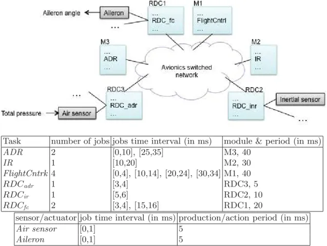
Let us consider an avionics case study depicted in Figure 1. This case study is a part of a flight control system (FCS).
System Description. The functional chain under analysis can be summerized as follows: the Air sensor periodically measures the total air pressure outside the aircraft (TPana). This analog value is digitalized (TPdig) and transmitted
through a Remote Data Concentrator RDCadr to the Air Data Reference
func-tion (ADR). The ADR computes the speed of the aircraft (speed1) and sends
it to the Intertial function (IR) which consolidates the data with data from an inertial sensor. The consolidated speed (speed2) is then returned to the ADR
for validation which sends the final speed value (speed3) to the Flight controller (FlightCntrl). It computes the angle (θdig) which must by applied to the aileron.
This last data is transmitted to the aileron actuator (Aileron) through RDCfc.
Finally, Aileron transforms the digital data θdig into a physical angle (θana).
This functional chain is formalized as F =TP→ Air sensorφ TP→ RDCdig adr TPdig → ADR speed1 → IR speed2 → ADR speed3 → FlightCntrl θ→ RDCdig fc θdig → Aileron θana → . The architecture of the system and the real-time parameters are depicted in figure 1. System Requirements. The chain F must satisfy the requirements:
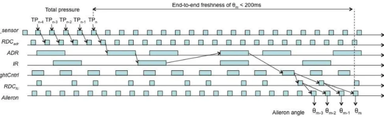
– (200ms)-freshness: at any time, the aileron angle θ must correspond to
a total air pressure measured at most 200ms before. This is illustrated in figure 2 and analyzed in section 4.
– (300ms)-reactivity: any variation of air pressure longer than 300ms must reflect on the angle applied to the aileron. This is analyzed in section 5.
3
The Analysis Approach: Overview
The analysis method is based on two steps: (1) simplification of the system by abstracting the network with a set of timed channels, and (2) evaluation of the worst case end-to-end freshness (WCF) or worst case end-to-end reactivity.
Task number of jobs jobs time interval (in ms) module & period (in ms) ADR 2 [0,10], [25,35] M3, 40 IR 1 [10,20] M2, 30 FlightCntrk 4 [0,4], [10,14], [20,24], [30,34] M1, 40 RDCadr 1 [3,4] RDC3, 5 RDCir 1 [5,6] RDC2, 10 RDCfc 2 [3,4], [15,16] RDC1, 20
sensor/actuator job time interval (in ms) production/action period (in ms)
Air sensor [0,1] 5
Aileron [0,1] 5
Fig. 1. Case-study: a flight control subsystem
First step: abstraction of the network The combinatorial complexity of the veri-fication of real-time properties takes its root in the asynchronism of the modules, and indeterministic congestion in the network. We showed in [LEPB10] that tak-ing into account all these factors in the evaluation of end-to-end properties is intractable. However, in the area of distributed embedded systems, the traversal time of each message through the network from one module to another one must bounded. The complexity of our analysis method can be significantly reduced by abstracting the network with a set of timed channels. In this setting, each communication is abstracted with a channel characterized by a time interval [δmin, δmax], where δmin (resp. δmax) is the lower (resp. upper) bound of the
network traversal time along the path. As said in section 1.3, these bounds can be determined with various formal methods, depending on the nature of the network. For instance, the trajectory approach has been successfully applied to switched embedded networks in [BSF09]. The Network Calculus [LBT01] method has been extended to switched networks with several priorities level [SB12]. Simi-larly, [HHKG09, CB10, FFF11] propose methods for evaluating lower and upper bounds of communication delays in other classical real-time networks such as CAN, Flexray, and SpaceWire. Generally speaking, these methods involve the communication path parameters (route in the network, throughput of the net-work nodes, maximum size of the messages allocated to the path,. . . ), and they associate each path with its minimal and maximal traversal time. We do not
Fig. 2. A end-to-end freshness requirement in the flight control system
describe these analysis techniques in the following. Readers interested in worst case traversal times analysis are invited to consult the provided references.
By way of example, in the FCS case study we consider that each communica-tion is abstracted by a timed channel [1, 3] (in ms): each frame undergoes a delay between 1ms and 3ms to reach its destination. Note that this abstraction is an over-approximation because the bounds of the timed channels are determined with Network Calculus, which is an over-approximative technique. We discuss the significance of this point through experiments in section 6.
Second step: freshness and reactivity evaluation This second step constitutes the contribution of the article. It is based on an abstract model where the network and the communication paths are replaced by timed channels, and on linear programing. The idea is to characterize all the possible behaviors along a func-tional chain with a set of variables and constraints, and afterwards to determine the worst case scenario among all these possible behaviors with respect to the property under analysis. One of the advantage of this approach is that finding the worst case scenario can be done automatically by a solver.
4
Worst-Case End-to-End Freshness Analysis
As previously stated, we model the behavior of each element by a set of variables and constraints. The behavior of the whole system is obtained as the conjunction of all these constraints. This defines a Mixed Integer Linear Program (MILP) which can be used to determine the worst case freshness of a functional chain. In the following, all variables used for offsets and dates are reals. All variables used to designate a specific hyper-period or a job are integers. Although not mandatory, we only use integers for parameters in order to improve readability.
4.1 Modeling
Module. Let Mi be a module. The only variable which characterizes Mi is its
possible offset with respect to the other modules. Modules are asynchronous, thus the time origin of their execution frame may be shifted by an offset Oi.
This offset may be arbitrary. However, as we are interested in the regular be-havior, and not the specific case of the initialization phase, it is not necessary to
consider offsets greater than the maximal hyper-period of the system. The first constraints for Mi are then:
Oi ∈ R, 0 ≤ Oi ≤ maxk=0...mHk
Task (Including Sensor and Actuator). Tasks are the only active
ob-jects of our modeling. Let τj be a task running on the module Mi. Let d be
a data periodically produced by τj. The task τj is characterized by a set of jobs
τj(k) for k = 0 . . . nj. τj(k) is the kth job of τj in the hyper-period Hi. Each job
is characterized by a time interval [bj(k), ej(k)]. These dates are relative to the
beginning of the current hyper-period which is itself relative to the start of mod-ule Mi. Then, if n is the number of the current hyper-period, the absolute time
interval corresponding to the job τj(k) is [Oi + nHi+ bj(k), Oi + nHi+ ej(k)].
Let us suppose that another task reads the output data d produced by τj at
tread (tread is an absolute date). To evaluate the possible freshness of d at tread,
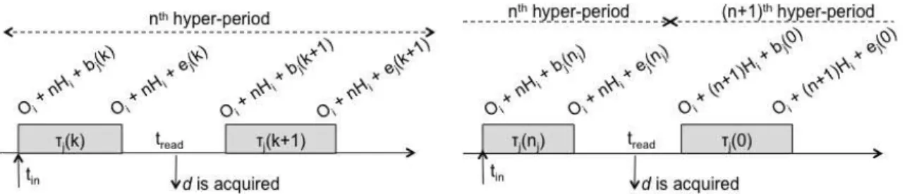
one has to determine which job has produced d. This job is characterized by its index k and the index n of its hyper-period satisfying the following constraints
Oi+ nHi+ bj(k) ≤ tread <Oi+ nHi + ej(k + 1)
for k < nj, i.e., the job is not the last job of τj in the nth hyper-period, as shown
in the figure 3(a). And
Oi + nHi+ bj(nj) ≤ tread <Oi + (n + 1)Hi + ej(0)
for k = nj, i.e., the job is the last job of τj in the nth hyper-period, as shown
in the figure 3(b). In other terms, in the first case (left part of the figure), if d is acquired after (the relative date) bj(k) and strictly before ej(k + 1), it is
possibly produced by the kth job; indeed τ
j(k) may produce d anywhere in its
time interval, then possibly at Oi+ nHi+ bj(k), and similarly τj(k + 1) may take
all its time interval for producing a new data, then possibly at Oi+nHi+ej(k+1).
The second case is similar.
Then, if we consider all the jobs of τj, determining the job and the
hyper-period producing d could be done simply by considering a set of boolean variables Bk k = 0 . . . nj (one variable per job) such that one and only one Bk is true
∀k = 0 . . . nj, Bk ∈ {0, 1}, Pk=0...njBk = 1
and such that the two following constraints are true: (
tread <Oi + nHi+
P
k=0...(nj−1)Bk· ej(k + 1) + Bnj(Hi + ej(0))
Oi+ nHi +Pk=0...njBk · bj(k) ≤ tread
For a given offset of the module Oi and for a given tread (acquisition date of d),
these two constraints determine a set of couples (n, k), i.e., a set of jobs which can produce d. Note that the solution is note unique because of the variation of the execution time of each job.
(a) first case: d is acquired between two jobs from the same hyper-period
(b) second case: d is acquired between two consecutive hyper-periods
Fig. 3. Rules determining which job has produced the data d acquired at tread
Then, for any couple of hyper-period n, and job k, which respects the previous constraints, only one acquisition date (tin) of the input related to the occurrence
of d is acceptable. It it constrained by the beginning of the job: tin= Oi+ nHi +Pk=0...njBk · bj(k)
Recall that only one of the Bk is true and denotes the job producing d; then
P
k=0...njBk · bj(k) is the relative date at which the related input is acquired.
The local freshness of d at time tread is then tread− tin.
Communication through a Timed Channel. Let us now consider a timed channel characterized by a communication time in [δmin, δmax] and a data d
crossing that timed channel. If tbefore and tafter are the input and the output
dates of d from the channel, then tbefore and tafter are related by
tafter− δmax ≤ tbefore ≤ tafter− δmin
Communication through a Shared Memory. Tasks on a same module communicate through the local shared memory and requires no time. A shared memory is similar to a channel characterized by the interval [0, 0]:
tafter = tbefore
4.2 Worst-Case Freshness on the Whole System
Let → τin n an → . . . τ1 a1 → τ0 out
→ be a functional chain. The model of this chain is simply obtained by connecting all the constraints of all the jobs and the communication involved in the chain. The set of constraints thus obtained forms a MILP. Let us note touta date at which the final output out is observed, and tin
the related acquisition date of the input parameter in. tout and tin are related
by the set of the previous constraints. Then the freshness of out at tout is
F = tout− tin
The worst case latency is obtained on a particular behavior maximizing F . This behavior can be found by using a MILP solver with the objective function:
4.3 Application to the Case-Study
Consider the functional chain in Figure 2. The global MILP model obtained for analyzing the worst case freshness of the chain is composed of 42 constraints and 43 variables. As an example, we only give here the beginning of the model, concerning the end of the chain, i.e., the actuator Aileron, and the communica-tion task RDCfc on RDC1. The modeling language used in this listing is the one
used for lp_solve [BEN04] input files.
max : t0 - t8 ; // freshness expression to maximize // Module offsets
OAileron <= 40; ORDC1 <= 40; OM1 <= 40; OM2 <= 40; OM3 <= 40; ORDC3 <= 40; OAir_sensor <= 40; // Timed channels bounds
deltamin = 1; deltamax = 3;
// Aileron model where t0 is the date of the aileron angle t0 < OAileron + 5 nAileron + 6; t0 >= OAileron + 5 nAileron + 0; t1 = OAileron + 5 nAileron + 0;
// From RDC_fc to Aileron
t1prime >= t1 - deltamax; t1prime <= t1 - deltamin; // RDC_fc t1prime < ORDC1 + 20 nRDC1 + 16 B1RDC_fc + 24 B2RDC_fc ; t1prime >= ORDC1 + 20 nRDC1 + 3 B1RDC_fc + 15 B2RDC_fc ; B1RDC_fc <= 1 ; B2RDC_fc <= 1; B1RDC_fc + B2RDC_fc = 1; t2 = ORDC1 + 20 nRDC1 + 3 B1RDC_fc + 15 B2RDC_fc; // From FlightCntrl to RDC_fc
t2prime >= t2 -deltamax; t2prime <= t2 - deltamin; ...
The MILP is solved with lp solve in less than 1s on a 2.53 GHz processor. The maximal freshness returned for the case-study is 175ms. Hence, the system satisfies the (200ms)-freshness requirement.
5
Worst-Case End-to-End Reactivity Analysis
The second property we are interested in is the reactivity of a functional chain to an input signal. Let us consider again the case study figure 2. Imagine a gust of duration δms. The consequence of this gust is to suddenly increase the value of the total pressure at the input of the system. Let us suppose that for aerodynamical reasons the system has to react to any gust of duration δ is greater that 300ms; briefer gust may be ignored. Then one has to verify that it is never the case that all total pressure samples during any window greater than 300ms are lost (i.e., overwritten) somewhere in the chain, and then do not impact the aileron angle computation. For instance, in the scenario figure 2, samples T Pn−4
to T Pn−1 are overwritten by T Pn, and then are lost. The period of Air sensor
is 5ms. Then it comes directly from this scenario that the chain is not reactive to gusts of duration 20ms. The question is: can we determine the worst case end-to-end reactivity of this chain?
Fig. 4. a non δ-reactivity case
5.1 δ-Reactivity Modeling
Let us consider a functional chain→ τin n an
→ . . . τ1 a1
→ τ0 out→. The chain is δ-reactive
if and only if in any window [t, t + δ], at least one sample of in is related to a sample of out. Conversely, the chain is not δ-reactive if and only if they are two consecutive output samples outk and outk+1 which depend respectively from two
input samples inm and inm′ such that inm and inm′ are separated by more than
δ time units. In that case, as shown in figure 4, any sample inp acquired after
inm and before inm′ is lost, overwritten by inm′ somewhere in the chain.
Following this idea, a simple way to verify a chain is δ-reactive is:
1. Consider two consecutive output samples outk and outk+1. For the sake of
simplicity, let us suppose that τ0 is a task composed of only one job, an
actuator of period T0 for instance. As τ0 is the last task in the chain, its
processing time does not impact the reactivity. Thus, to simplify the evalu-ation of the reactivity of the chain, it is not necessary to consider dates of each sample outk and outk+1. It is sufficient to consider the beginning date
of there respective jobs. Let tk
0 and tk+10 be these dates:
tk0 = O0+ k · T0 and tk+10 = O0+ (k + 1) · T0
To generalize to task τ0 composed of several jobs can be done simply by
following the modeling presented in the previous section. 2. Determine the dates tm
n and tm
′
n , i.e., the dates of the inputs related to ok
and ok+1 (i.e., in figure 4, inm and inm′). This analysis is done by using the
constraints presented in the previous section.
3. Determine the reactivity related to (outk,outk+1) as the difference between
these two input dates: reactivity(outk,outk+1) = tm
′
n − tmn. The chain is then
δ-reactive if
∀k, reactivity(outk,outk+1) ≤ δ
As previously, the worst case reactivity is obtained on a particular behavior maximizing reactivity(outk,outk+1), for any k. This behavior can be found by
using a MILP solver with the objective function: maximize: tm′
5.2 Application to the Case-Study
Consider the functional chain in Figure 2. The global MILP model obtained for analyzing the worst case reactivity of the chain is composed of 95 constraints and 75 variables. As an example, we only give here the beginning of the model, con-cerning the end of the chain, i.e., the actuator Aileron, and the communication task RDCfc on RDC1.
max : r8 - t8 ; // reactivity expression to maximize // Offsets
OAileron <= 40; ORDC1 <= 40; OM1 <= 40; OM2 <= 40; OM3 <= 40; ORDC3 <= 40; OAir_sensor <= 40; // Timed channels bounds
deltamin = 1; deltamax = 3;
// First sample at t0 produced by the job ntAileron // *******************
// Aileron
t1 = OAileron + 5 ntAileron; // From RDC_fc to Aileron
t1prime >= t1 - deltamax; t1prime <= t1 - deltamin; // RDC_fc t1prime <= ORDC1 + 20 ntRDC1 + 16 B1tRDC_fc + 24 B2tRDC_fc ; t1prime > ORDC1 + 20 ntRDC1 + 3 B1tRDC_fc + 15 B2tRDC_fc ; B1tRDC_fc <= 1 ; B2tRDC_fc <= 1; B1tRDC_fc + B2tRDC_fc = 1; t2 = ORDC1 + 20 ntRDC1 + 3 B1tRDC_fc + 15 B2tRDC_fc; ...
// second sample at r0 produced by the job nrAileron // *******************
// Aileron
nrAileron = ntAileron + 1 ; r1 = OAileron + 5 nrAileron; // From RDC_fc to Aileron
r1prime >= r1 - deltamax; r1prime <= r1 - deltamin; r1prime >= t1prime ; // RDC_fc r1prime <= ORDC1 + 20 nrRDC1 + 16 B1rRDC_fc + 24 B2rRDC_fc ; r1prime > ORDC1 + 20 nrRDC1 + 3 B1rRDC_fc + 15 B2rRDC_fc ; B1rRDC_fc <= 1 ; B2rRDC_fc <= 1; B1rRDC_fc + B2rRDC_fc = 1; r2 = ORDC1 + 20 nrRDC1 + 3 B1rRDC_fc + 15 B2rRDC_fc; r2 >= t2 ; ...
The MILP is solved with the solver lp solve in 140s on a 2.53 GHz processor. The maximal reactivity returned for the case-study is 130ms.
6
Discussion: Global versus Local Approach
6.1 Freshness Analysis: Local versus Global Approach
To evaluate the gain we may achieve, we benchmark our global approach against a local one. As described in section 1.3, a local approach consists in determining the local worst case freshness (LWCF) of each component visited in the func-tional chain with respect to the previous component only. Then the end-to-end
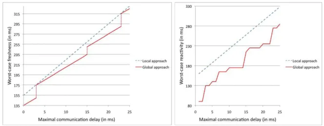
(a) Worst-case freshness: local versus global approach
(b) Worst-case reactivity: local versus global approach
Fig. 5.Local versus global approach
freshness is the sum of each LWCF. The LWCF of a timed channel is the upper
bound of the communication delay: δmax. In the same way, the LWCF of a task
τi is the maximal delay between the begin and the end of two consecutive jobs
(i.e., the time for a data to be refreshed). Then, in our case study, the end-to-end freshness obtained following this local reasoning is:
LF = 6 + 13 + 14 + 35 + 40 + 35 + 6 + 6 + 7δmax = 155 + 7δmax (in ms) (1)
Figure 5(a) compares the local and global approaches by varying δmax.
Accord-ing to equation (1) the worst case freshness determined with the local approach is linear (straight dashed line). The results of the global approach form a step linear function and gives more accurate results than the local approach. The curve of the global approach varies by steps because the functional chain crosses
module M3 twice. System designers could take advantage of this more accurate
evaluation technique: within certain range they could increase the network load with lower impact on the end-to-end freshness than predicted by the local ap-proach. For instance, the curves figure 5(a) show that for a maximal traversal
time through the network δmax = 7ms, the global WCF is equal to 195ms while
the local one is 204ms. Put differently, only the global method shows that the chain still meets the requirement.
6.2 Reactivity Analysis: Local versus Global Approach
We compare our global reactivity analysis with a local approach. The reactivity obtained following a local method is the difference between the maximal fresh-ness LF and the minimal freshfresh-ness plus one period of the end task of the chain τ0. Following only a local reasoning, the minimal freshness happens when the
network traversal time is minimum (δmin ) and when all tasks take no time and
are well phased. Thus in our case study the end-to-end reactivity is:
LR= 155 + 7(δmax− δmin) + 5 = 160 + 7(δmax− δmin) (in ms) (2)
We compare again the global approach against the local one by varying δmax
(δmin remains equal to 1ms). The results are plotted on figure 5(b). According
to equation (2) the worst case reactivity determined with the local approach is linear (straight dashed line). The results of the global approach form a more complex curve and gives more accurate results.
7
Conclusion
The article presents an analysis method for end-to-end freshness/reactivity prop-erties on GALTT systems. This verification method is based on a MILP model-ing. Worst case end-to-end properties are computed as optimal solutions of the MILP problem. An interesting feature of this approach is that one can easily compute best case end-to-end properties. It only requires to modify the objec-tive function of the MILP form max to min. From a scalability point of view, the case study considered previously is composed of 7 tasks (including the sensor, the actuator, and the communication tasks), one of them (ADR) being crossed two times. This case study is representative from industrial systems (usually composed of 5 to 10 tasks). Our method applied to this case study does not take more than 1s for the freshness analysis and 140s for the reactivity analysis (with a non optimized solver). We think that these results are promising.
In this article, we made however a strong hypothesis about the internal be-havior of the tasks. We implicitly considered that each job of each task does not induce a delay greater than its worst case response time, i.e., the length of its time interval. This implicit hypothesis is shown figure 2 where each job returns an output data before the end of its time interval. Obviously it is not always the case in realistic systems. Some tasks can implement “confirmation tests” waiting for a given amount of time (generally a multiple of its period) before producing a consolidated output. Obviously this internal latency impacts the global latency and the global reactivity of the chain. Our next work to do is to extend our global method by tasks involving internal delays.
References
[ARI97] ARINC 653, Aeronautical Radio Inc.: Avionics Application Software Standard Interface (1997)
[BD12] Boyer, M., Doose, D.: Combining network calculus and scheduling theory to improve delay bounds. In: RTNS 2012, pp. 51–60 (2012)
[BEN04] Berkelaar, M., Eikland, K., Notebaert, P.: lp solve 5.5, open source (mixed-integer) linear programming system. Software, (May 2004), http://lpsolve.sourceforge.net/5.5/
[BSF09] Bauer, H., Scharbarg, J.-L., Fraboul, C.: Applying and optimizing tra-jectory approach for performance evaluation of afdx avionics network. In: Proceedings of the 14th IEEE International Conference on Emerging Technologies & Factory Automation, ETFA 2009, Piscataway, NJ, USA, pp. 690–697. IEEE Press (2009)
[CB06] Carcenac, F., Boniol, F.: A formal framework for verifying distributed embedded systems based on abstraction methods. International Journal on Software Tools for Technology Transfer 8(6), 471–484 (2006)
[CB10] Chokshi, D.B., Bhaduri, P.: Performance analysis of flexray-based sys-tems using real-time calculus. In: Shin, S.Y., Ossowski, S., Schumacher, M., Palakal, M.J., Hung, C.-C. (eds.) SAC, pp. 351–356. ACM (2010) (revisited)
[FFF11] Ferrandiz, T., Frances, F., Fraboul, C.: Worst-case end-to-end delays eval-uation for spacewire networks. Discrete Event Dynamic Systems 21(3), 339–357 (2011)
[HHKG09] Herpel, T., Hielscher, K.-S.J., Klehmet, U., German, R.: Stochastic and deterministic performance evaluation of automotive can communication. Computer Networks 53(8), 1171–1185 (2009)
[LBEP11] Lauer, M., Boniol, F., Ermont, J., Pagetti, C.: Latency and freshness anal-ysis on IMA systems. In: Emerging Technologies and Factory Automation (ETFA), Toulouse, France. IEEE (September 2011)
[LBT01] Le Boudec, J.-Y., Thiran, P.: Network Calculus. LNCS, vol. 2050. Springer, Heidelberg (2001)
[LEPB10] Lauer, M., Ermont, J., Pagetti, C., Boniol, F.: Analyzing end-to-end func-tional delays on an IMA platform. In: Margaria, T., Steffen, B. (eds.) ISoLA 2010, Part I. LNCS, vol. 6415, pp. 243–257. Springer, Heidelberg (2010)
[MM06] Martin, S., Minet, P.: Worst case end-to-end response times of flows sched-uled with FP/FIFO. In: Proceedings of the International Conference on Networking, International Conference on Systems and International Con-ference on Mobile Communications and Learning Technologies, pp. 54–62. IEEE Computer Society, Washington, DC (2006)
[SAA+
04] Sha, L., Abdelzaher, T., AArz´en, K.-E., Cervin, A., Baker, T., Burns, A., Buttazzo, G., Caccamo, M., Lehoczky, J., Mok, A.K.: Real time schedul-ing theory: A historical perspective. Real-Time Syst. 28(2-3), 101–155 (2004)
[SB12] Mangoua Sofack, W., Boyer, M.: Non preemptive static priority with net-work calculus: Enhancement. In: Schmitt, J.B. (ed.) MMB & DFT 2012. LNCS, vol. 7201, pp. 258–272. Springer, Heidelberg (2012)
[Spu96] Spuri, M.: Holistic Analysis for Deadline Scheduled Real-Time Distributed Systems. Research Report RR-2873, INRIA (1996)
[TC94] Tindell, K., Clark, J.: Holistic schedulability analysis for distributed hard real-time systems. Microprocessing and Microprogramming 40(2-3), 117–134 (1994)
[TCN00] Thiele, L., Chakraborty, S., Naedele, M.: Real-time calculus for scheduling hard real-time systems. In: ISCAS, pp. 101–104 (2000)