HAL Id: insu-03234754
https://hal-insu.archives-ouvertes.fr/insu-03234754
Submitted on 25 May 2021
HAL is a multi-disciplinary open access
archive for the deposit and dissemination of
sci-entific research documents, whether they are
pub-lished or not. The documents may come from
teaching and research institutions in France or
abroad, or from public or private research centers.
L’archive ouverte pluridisciplinaire HAL, est
destinée au dépôt et à la diffusion de documents
scientifiques de niveau recherche, publiés ou non,
émanant des établissements d’enseignement et de
recherche français ou étrangers, des laboratoires
publics ou privés.
Complete wave-vector directions of electromagnetic
emissions: Application to INTERBALL-2 measurements
in the nightside auroral zone
O Santolik, François Lefeuvre, Michel Parrot, Jean-Louis Rauch
To cite this version:
O Santolik, François Lefeuvre, Michel Parrot, Jean-Louis Rauch. Complete wave-vector directions
of electromagnetic emissions: Application to INTERBALL-2 measurements in the nightside auroral
zone. Journal of Geophysical Research Space Physics, American Geophysical Union/Wiley, 2001, 106,
pp.13191-13201. �insu-03234754�
JOURNAL OF GEOPHYSICAL RESEARCH, VOL. 106, NO. A7, PAGES 13,191-13,201, JULY 1, 2001
Complete wave-vector directions of electromagnetic emissions:
Application to INTERBALL-2 measurements
in the nightside
auroral zone
O. Santol•, •,2 E Lefeuvre, M. Parrot, and J. L. Rauch
Laboratoire de Physique et Chimie de l'Environnement, Centre National de la Recherche Scientifique, Orltans, France.
Abstract. We present several newly developed methods for wave propagation analysis. They are based on simultaneous measurement of three magnetic field components and one or two electric field components. The purpose of these techniques is to estimate complete wave vector direction and the refractive index. All the analysis results are validated by well defined simulated data. Propagation analysis of natural emissions in the night-side auroral zone at high altitudes is done using the data of the MEMO (Mesures Multicomposantes des Ondes) experiment onboard INTERBALL-2. The results show that a bursty whistler mode emission propagates toward the Earth near the resonance cone. Upward propagating auroral kilometric radiation in the R-X mode represents another example demonstrating the potential of such analysis for future applications.
1. Introduction
With multicomponent wave measurement onboard satel- lites, the wave vector direction may be determined using the Faraday's law. Its consequence in the frequency domain is the perpendicularity of the magnetic field vector B to both the wave vector k, and the electric field vector E. The mag- netic field data are often used to characterize k [e.g., Means,
1972; McPherron et al., 1972; Samson and Olson, 1980].
The wave vector direction is here defined by the normal to the polarization plane of the magnetic field. If the polariza- tion is circular or elliptic, two mutually antiparallel direc- tions always meet this condition. The result is thus ambigu- ous, and the wave vector direction can only be determined in a single hemisphere. The complete wave vector direc- tion without this ambiguity may be however determined if we measure both the magnetic field and the electric field [Lefeuvre et al., 1986]. To fully define the wave vector,
can be reduced to five in the case of a plane wave [Grard, 1968; $hawhan, 1970].
Sometimes, the wave propagation cannot be well de- scribed by a single direction. For instance, it is the case when foregoing and reflected waves are simultaneously ob- served [e.g., Lefeuvre et al., 1992; Santol& and Parrot, 2000] or when several propagation modes coexist [e.g., Parrot et al., 1989]. Then the wave propagation may be described by
means of the wave distribution function (WDF) introduced
by Storey and Lefeuvre [1979]. However, the quasi-plane wave approximation is often valid when a direction or/and
a mode is dominant. Even if the field is not exactly con-
sistent with this assumption, an estimate of the plane wave parameters may represent an average value for all simulta- neously propagating waves and give a rough idea about the wave propagation.
The electric field data available from satellite measure-
ments are often incomplete: only one or two electric com-
we also need to determine
its modulus,
the wave number ponents
may be available.
Approximations
may be used
for
k. This, again, cannot be done without considering the wave electric field components. A nonambiguous determination of the propagation characteristics of a wave is of crucial im- portance for the location of the source and the identification of the generation mechanism of plasma waves. In theory, it requires the measurement of six electromagnetic field com- ponents (three electric and three magnetic), and the number
1Also at Faculty of Mathematics and Physics, Charles University,
Prague, Czech Republic.
9•Now at Department of Physics and Astronomy, University of Iowa,
Iowa City.
Copyright 2001 by the American Geophysical Union. Paper number 2000JA000275.
0148-0227/01/2000JA000275509.00
particular orientations of electric antennas as regards to the Earth magnetic field direction [Lefeuvre et al., 1986]. In the other cases, specific analysis methods must be developed. The difficulty is that the electric and magnetic wave field components being related through the refractive index, i.e., through the dispersion relation, approximations valid in one region of the Clemmow-Mullaly-Allis (CMA) diagram [Stix, 1992] do not apply to others. This explains why techniques which have been proved to be successful for the analysis of some satellite data (e.g., techniques developed by Santol& and Parrot [1998, 1999] for the extremely low frequency data of the FREJA satellite) must be reexamined for other
data.
In this paper, analysis techniques are used under the plane wave approximation, and for an incomplete set of data. We revise these methods in the context of the INTERBALL-
13,192 SANTOL•K ET AL.' WAVE-VECTOR DIRECTIONS IN THE NIGHTSIDE AURORAL ZONE
2 waveform data, with a potential application to the data of the STAFF (Spario-Temporal Analysis of Field Fluctua- tions) spectral analyzer onboard the European Space Agency CLUSTER satellites. Two sets of INTERBALL-2 observa- tions made in November 1996, at nearly the same position (nightside, northern auroral region), are used as an exam- ple of investigation of propagation characteristics of bursty whistler mode emissions and auroral kilometric radiation (AKR). These emissions were mainly studied using the fre- quency power spectrograms in the past. We will show that multicomponent data, as recorded onboard INTERBALL 2 [Lefeuvre et al., 1998], allow a more detailed analysis. Sec- tion 2 introduces the analysis methods, and in section 3 we
show the results for the INTERBALL-2 data in two differ- ent frequency bands. Each case is compared with theoretical predictions adjusted to the particular experimental situation. Section 4 contains a discussion of results, and, finally, sec- tion 5 gives brief conclusions.
2. Analysis Methods
Analysis of electric field data in space plasmas may suf- fer from several problems. The first problem is the coupling impedance between the antennas and the plasma which of- ten is poorly known and which may shift the phase or change the amplitude of the signal. These effects depend on param-
eters which are difficult to control on board and which are
more or less well modeled. The second problem is the diffi- culty to install a long antenna in the direction of the satellite spin axis and so to get accurate measurements of the three components. The third problem exists if, owing to telemetry limitations, the waveform of a single electric field compo-
nent is transmitted. This is the case of INTERBALL 2 data
in the highest frequency band (20- 200 kHz).
It is therefore important to have methods which (1) char- acterize the complex transfer function (the phase shift and the change of amplitude) directly from the wave data, (2) es- timate the hemisphere of propagation to complete the wave vector direction, (3) estimate the wave number, and (4) are able to work with incomplete electric field data, i.e., with measurements of only one or two electric components. The full vector measurement of the wave magnetic field is sup- posed. Several methods meeting some of these points are
described in this section.
The basic equation used by all the analysis methods is the Faraday's law,
0B
V x E-
Or'
(1)
All the methods work in the frequency domain. The mul- ticomponent data are first subjected to a cross-spectral anal- ysis. At each analyzed frequency, the result of this procedure is a Hermitian spectral matrix,
where Ai and Aj are the complex
amplitudes
of ith and
jth signal obtained by a classical spectral analysis [e.g., Priestley, 1989], the asterisk stands for the complex conju-
gate, and () mean the time average. Autopower spectra of separate signals may be found on the main diagonal of the spectral matrix. Its off-diagonal elements are complex cross spectra between each two signals, giving information about mutual phase and coherency relations.
2.1. Analysis Using the Magnetic Field Vector Data Although the subject of the present paper is a simulta- neous analysis of the magnetic and electric fields, we will
also need three auxiliary procedures based only on the mag- netic field vector measurements. Methods of direction find- ing with these data [e.g., Means, 1972; McPherron et al.,
1972; Samson and Olson, 1980] are based on the perpendic- ularity of the wave vector to the wave magnetic field,
B. k - 0,
which is is a consequence of (1) in the frequency domain. In this paper we will use the method of Means [1972]. It con- sists of a straightforward algebraic expression using imag- inary parts of three magnetic cross spectra and gives esti- mates of angles 6• and •b which characterize the wave vector direction in a spherical coordinate system. Owing to the am- biguity noted in section l, we cannot distinguish two oppo- site directions. We may thus choose to represent the results in the hemisphere where 6• _< 90 ø. It is also useful to trans- form the wave magnetic data into a system whose z axis is parallel to the ambient magnetic field (B0). Obviously, this
transformation needs the full vector measurements. Polar
angle 6• then defines the angle deviation from the ambient DC magnetic field, and angle •b gives the azimuth having the zero value in the direction of increasing magnetic lati- tude. The method always gives an ambiguous result with 0 _< 90 ø, which may also indicate an antiparallel propaga- tion with 0' - 180ø-0 and •b' - 180 ø +•b.
We will also use an estimate of the sense of circular or
elliptical polarization in the plane perpendicular to B0,
C• -
a(.•S•y)
'
(4)
where .•S•y is the imaginary part of the cross spectrum between the two perpendicular magnetic components, and
gr(.,•Sa:y
) -- V/(Sa:a:Syy
-- •}•Sx2y
-•-
.,•$•y)
/ V/(2M)
is an
esti-
mate
of its standard
deviation
[Priestley,
1989].
Here,
•S•y
is the real part of this cross
spectrum,
S• and Syy are the
corresponding autospectra, and M is the number of matrices entering into the average in (2). With the convention we use for the spectral analysis, negative values of Cs mean left- hand polarized waves (sense of the gyration of ions) and pos- itive values correspond to right-handed polarization (sense of the gyration of electrons). The absolute value gives the level of confidence, and values above 3 or below -3 gener- ally indicate a high confidence level.
The underlying hypothesis on the presence of a single plane wave will be tested by an estimator of the degree of polarization obtained by the eigenanalysis of the spectral matrix [Samson, 1977; Storey et al., 1991; Lefeuvre et al.,
SANTOL[K ET AL.' WAVE-VECTOR DIRECTIONS IN THE NIGHTSIDE AURORAL ZONE 13,193
v3
P = Vx
+ V2
+ V3'
(5)
where V•, V2, and V3 are three real eigenvalues of the spec- tral matrix 3 x 3 of the three magnetic components, V3 being the largest one. A value above •0.8 means that the wave
magnetic
field approximately
corresponds
to that of a single
plane wave.
2.2. Estimations From the Magnetic Field Vector Data and a Single Electric Signal
As noted in section 1, the two opposite wave vector di- rections may be distinguished if we use both magnetic and electric field data. We must obviously know the direction of the electric antenna in the coordinate system, which is used for the components of the wave magnetic field vector data,
i.e., in the Bo frame. Even if more than one electric antenna is available, it can be useful to check that similar results are
independently obtained for each electric signal. With a sin- gle electric antenna, two approximate methods can be used. The first possibility is to determine the phase shift between the electric signal and a magnetic component Ba = Pa' B. This component is calculated as a projection of the magnetic field vector to a unit vector Pa = • x a, perpendicular to both a unit vector a in the direction of the
electric antenna and the z axis of the Bo coordinate system
[Santol& and Parrot, 1999]. Using the cross spectrum Sxa between the x component of the magnetic field and the elec- tric signal (i.e., the component of the electric field along the antenna axis), together with the cross spectrum $ua between the magnetic y component and the same electric signal, we
have
SBa
-
-
+
-
= ISBI exp(i(I'a), (6)
nations of wave mode, frequency, and/or wave vector direc- tion (for example, the whistler mode emissions presented by
Santoh7c and Parrot [ 1999]). Note that the transfer function
of the antenna-plasma interface may have a nonzero imagi- nary part. In such a case it induces a phase shift to the elec- tric signal. This phase shift is then directly reflected by • as an additive value. This may complicate the analysis, but under some circumstances the method may also serve to es-
timate the unknown transfer function.
If the electric field vector is parallel to the antenna di- rection, the above procedure might also be used in the de- termination of the sign of the z component of the Poynting vector (Fz). Another, closely related, method may be used to estimate Fz normalized by its standard deviation, D = F•/a(F•). With a single electric antenna we would obtain D only if the electric field vector were parallel to the an- tenna direction. We can however make use of an approxi- mate estimation from real parts of the cross spectra between the electric signal and two perpendicular magnetic compo-
nents [Santoh7c and Parrot, 1998, 1999],
Da
=
RSyaaz
- RSzaay
(7)
where
cr(RSua)
and cr(R$•a) are estimates
of the standard
deviations of the respective cross spectra [Priestley, 1989].
Note that the "direction indicator" of Santoh7c and Parrot
[ 1998] was defined in that way that it is equivalent to -D•. Here, positive values of Da correspond to a positive z com- ponent of the Poynting vector. The absolute value of Da indicates the reliability of the result. If it is higher than 3, the interpretation of Da in terms of the sign of F• is sta- tistically reliable. All remarks made above concerning the interpretation of (I'a for the estimation of the k• sign are also
valid here.
where a• and a u are two components of the vector a in the Bo coordinate system. The phase shift is then defined by the complex phase (I'a of the complex scalar quantity Generally, • may have any value depending on the actual orientation of the antenna, on the unknown wave vector, and on the wave mode. In two special cases, however, •a di- rectly reflects the hemisphere of k: first, when the antenna direction lies in the plane perpendicular to k, and second, when the parallel component of the wave electric field (Ez) is negligible. In those cases, the phase shift •a is either 0 ø or 180ø: A phase shift around 180 ø corresponds to a posi- tive z component of the wave vector k• (0 < 90ø), and the zero value corresponds to a negative k• (0 > 90ø). If the procedure is continuously applied to the data of a spinning electric antenna, there are at least two points where the an- tenna intersects the plane perpendicular to k. If we know the k direction (e.g., from the method of Means [1972]) or if we are able to identify these points from the resulting time series, then in both these points we obtain • either 0 ø or 180 ø, and we can determine the hemisphere of prop- agation. Sometimes we can use this method continuously because of a negligible E•. This is true for some combi-
2.3. Analysis Using the Magnetic Field Vector Data and Two Electric Signals
With two electric antennas we can easily extend the pre- ceding method. We again suppose that we dispose of three magnetic components in the Bo frame and that in this frame we also know unit vectors a• and a2 defining the directions of the two electric antennas. These directions may or may not be mutually orthogonal. An extension of (7) then reads
Ei (•Syiaia: -- •Sa:iaiy)
Db
= Ei [ø'(•$yi)lai•:l
+ ø'(•$a:i)laiyl]
' (8)
where the index i goes from 1 to 2, for the first and the second electric antenna, respectively. Equation (8) repre- sents the sum of separate Fz estimates from (7) normal- ized by the sum of their standard deviations. This method gives an exact value of F•/crFz in the special case of two orthogonal electric antenna in the plane x-y (perpendicu- lar to Bo). The result indicates the correct sign of k• if kz(Sll -I-S22) > •}•SEzlkl -I-•SEz2k2, where $xx and o022 are the two electric autospectra, RSz• and RSE•2 are real parts of hypothetical electric crosspectra with the E• com-
13,194 SANTOL•K ET AL.: WAVE-VECTOR DIRECTIONS IN THE NIGHTSIDE AURORAL ZONE ponent and kx, k2 are the projections of the wave vector to
the directions of the two antennas. This condition is always valid if Ez is negligible but also in other cases depending on Ez, kl, and k2. Otherwise, interpretation of Db is similar as
in the case of Da. Note also that a further extension of (8) for
three orthogonal electric antennas may be obviously done by adding the third antenna to the sum, taking i = 1... 3. In this case, Db would always give the right value of Fz/a(Fz), independently of the directions of antennas, the wave vector,
terface. As we will make use of such data in (10), we must
take into account this transfer function. Suppose that the ith recorded electric signal œi may be written in the frequency domain as œi = Z Ei, where Z is a complex transfer func- tion at a given frequency (the same for all the antennas) and Ei is a theoretical electric component in the direction of the ith antenna. Then if we use experimental data in (10), we have a complex value N = n/Z on the left-hand side. Equa-
tion
(10) may
be finally
rewritten
to obtain
an estimate
of N
and the wave electric field. This method is thus important from the components of a spectral matrix,because of a relatively simple procedure and because it rep-
^'
^' + Sz'z)
½ (S•:jZ•:
q- SyjZy
resents
an
intermediate
step
between
the
method
(7) for
a
N-
(1
l)
single
antenna
and
a universal
procedure
for three
orthogo-
•, [($•j - $xy
cos
a)/sinai - •y,$tj '
nal electric antennas.
^• ^• and ^•
However,
with
two electric
antennas
we can
use
another
where
z•, zy,
z z are
Cartesian
components
of •.• in the
method to distinguish the two antiparallel wave vector di-rections without any assumption on the wave mode or on
the actual directions of antennas. At the same time we can
estimate the wave number. As a consequence of (1) in the frequency domain, we have
n (n x E) = cB, (9) where n is the index of refraction n = k c/ca, c is the speed of light, ca is the angular frequency, and n is a unit vector par- allel to the wave vector direction n - k/k. If we know n,
we can use it in (9) to estimate n (and then the wave number
k) from the measured electric and magnetic fields. Before using in (9), n may be determined by a method based on (3), for example by the method of Means [1972]. As such calcu- lation does not distinguish the two antiparallel wave vector directions, we have two possibilities: either the correct n is
introduced in (9), or -n is used. In the latter case, we obtain
-n instead of n, and, as n cannot be negative, we may use (9) to resolve the sign ambiguity of n.
The vector equation (9) may be written as three scalar equations in a Cartesian frame. Each equation necessarily contains two electric components from the vector product on the left-hand side. With two electric antennas we may use one of these scalar equations to determine n,
(lO)
original frame of the magnetic components, $xj, $uJ, and $zj are the cross spectra or autospectra between the mag- netic components Bx, By, and Bz and a fixed magnetic com- ponent (j is either x or y or z), and, finally, $xj and $•j are the cross spectra between the electric signals and the fixed magnetic component. The fixed component j may be arbi- trarily chosen between the three possibilities. Theoretically, the result should be the same whatever is the choice of j. In practice, a good choice to avoid numerical instabilities is to select j which gives the largest denominator in (11).
The resulting N may be decomposed to the complex am- plitude and phase,
n i•b
(12)
N-•e-
.
This shows that the wave refractive index cannot be sepa- rated from the absolute value of the transfer function I ZI, and we can only get a ratio of the two values from INI. The problem is that Z is often very poorly known, but in some cases, we can suppose that IZl is unity. The value of ISl - •/IZl then directly gives index of refraction n. At a given frequency f (f = ca/2•r), it also defines the wave- length of observed electromagnetic waves, ,• = c/nf.
If IZl is unknown, we can make use of theoretical values
of the refractive index, and the transfer function (and thus
the impedance of the electric antennas) may be estimated. Supposing that n has no imaginary part, the phase • di- The principal step of this method is thus the transforma- rectly reflects the phase shift due to the transfer function. tion of the three-component magnetic field data to get the
Bz, component in a Cartesian frame connected with the elec- tric antennas. The x' axis of this frame is parallel with a unit
vector a• in the direction of the first antenna. Its z • axis is
parallel to a unit vector • = a• x a2, perpendicular to both antennas. The y' axis completes the right-handed Cartesian
system,
lying in the plane
of the two antennas.
The compo-
nent
E u, then
reads
E u, = (E2 - E• cos
a)/sin a, where
cos c• = ax ß a2 characterizes the angle between the direc- tions of antennas. E• and E2 are the projections of the elec-
tric field vector
to the directions
of the two antennas,
respec-
tively. We always have E•, - E•, and if the antennas are
mutually
orthogonal,
we also
have
E
Experimental measurements of the electric field may be influenced by a transfer function of the antenna-plasma in-
As a secondary effect, this value may be used to resolve the sign ambiguity of n, as discussed above. Values below -90 ø or above +90 ø are equivalent to a negative real part of N. In this case, either the phase shift introduced by the trans- fer function is really so high and we use the right sign of n in (11), or the phase shift should be reduced by 180 ø and n has the opposite sign. If we have a reason to suppose that the antenna-plasma interface does not modify the phase by more than 90 ø , we may use the latter possibility to determine the sign of n.
Returning to (9) We may note that in the frequency do- main, the vectors of wave electric and magnetic fields are perpendicular. This property may be used to determine the full electric field vector from the measurement of three mag- netic and two electric components. The procedure must
SANTOLfK ET AL.: WAVE-VECTOR DIRECTIONS IN THE NIGHTSIDE AURORAL ZONE 13,195 again be based on the transformation to a coordinate frame
defined by the two electric antennas and is described in ap-
pendix
A. In this
paper
we use
such
completed
information
(a) about the wave electric and magnetic fields with two anal- .,ysis methods. The first one is an extension of the above
method
to estimate
the
normalized
parallel'
component
Of
the
Poynting vector (the Db parameter from (8), where the in- dex i'goes from 1 to 3). Its application to the three orth9go- ..nal electric components makes unnecessary all the additional Conditions of validity. The second method is based on a di- rect calculation of the angle deviation of the Poynting vector
F from
B0. This
angle
is obtained
without
any
ambiguity,
(c)
i.e. with values between 0 ø and 180 ø.
All the above presented data analysis methods are con-
tained
in the
computer
program
PRASSADCO
[Santoh7q
(d)
2000], which is being prepared for the STAFF-SA devices
onboard the CLUSTER satellites. The results shown in the
present
paper
have
been
obtained
by this
program.
3. Application to the MEMO Data in Two
Different Frequency Bands
The MEMO experiment [Lefeuvre et al., 1998] onboard
the INTERBALL
project
measures
the waveforms
of sev-
eral
components
of the
electromagnetic
field.
In its
ELF and
VLF bands (0.05-1 kHz and 1-20 kHz, respectively) it simul- taneously records the data from three magnetic antennas andtwo electric antennas. In its HF band (20-200 kHz) it mea-
sures
Waveforms
of three
magnetic
antennas
and
one
electric
antenna. We have selected two cases which will be analyzed with the above described methods. The data were respec- tively recorded in the ELF and HF bands of the MEMO de-vice.
3.1. Analysis of a Bursty Whistler-Mode ELF Emission
-r' 10-7. v
• 10-8
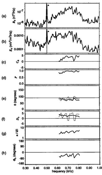
• o.oolo E (b) • E v "' 0.0001 (e) (f) (g) (h) o -5 1.o 0.5 0.0 150 100 50 0 5 -5 10 1 180 90 o -9o -180 0.30 ... i ... • ... , ... ! ... , ... i ... :;:;::;::1:::,::::: ::::::::::::::::::::::::::::::::::::::::::::::::: . ::::::::::::::::::::::::::::::::::::::::::::::::::::::::::::::::::::: ::::::::::::::::::::::::::::::::::::::::::::::::::::::::::::::::::::: 0.40 0.50 0.60 0.70 0.80 0.90 1.00 frequency (kHz)Figure 2. Analysis of a bursty ELF emission from Novem- ber 12, 1996, 1623:23 UT, in a frequency interval 0.3 - 1
The first case was recorded in the ELF band on Novem-
kHz. (a) Sum of the three magnetic autopower spectra. (b)
ber
12,
1996.
Figure
1 shows
a time-frequency
spectrogram
Sum
of the
two
electric
autopower
spectra.
(c)
Sense
of
of one
of the
electric
components
measured
between
1614
polarization
from
(4). (d)
Degree
of polarization
from
(5).
and 1625
UT. The data
were
organized
in short
snapshots
(e) Solid
line indictes
deviation
0 of the wave
vector
direc-
of 1.92
s separated
by ,.•63-s
data
gaps,
and
Figure
1 repre- tion from the ambient
magnetic
field B0 by the method
of
sents 10 snapshots separated by vertical lines. The satellite Means [1972] and dotted line indicates the same angle for
was
at an altitude
of 18,300
km in the nightside
northern
the
Poynting
vector
obtained
from
(A4). (f) Solid
line
de-
auroral
sector
at an invariant
latitude
of 68.5
ø and
around
notes
estimate
of the
normalized
parallel
component
of the
Poynting vector from (8) and dotted line denotes the same
0430
MLT
(magnetic
local
time).
In the
ninth
snapshot
of estimate
using
an
extension
of
(8)
for
three
electric
compo-
810. 6al.. . ' 242. 16 14:43 16 16:53 16 19:03 16 ai:13 16 23:23 16 24:30 UT
Figure 1. Power spectrogram of ten snapshots of the electric
field data recorded in the ELF band on November 12, 1996.
nents obtained using (A3). (g) Ratio of the wave refractive index and the transfer function from (12). (h) Phase shift due to the transfer function from (12).
this sequence, two similar bursts of natural waves were ob- served at frequencies around 700 Hz. Principal character-
istics
of the wave
propagation
are shown
in Figures
2a-2h.
Note that the vertical lines with asterisks in the frequency spectra (Figures 2a and 2b) identify disturbing interference signals with no relation to the observed phenomenon. These interferences are not seen in the electric component which is shown in Figure 1. The analysis is done only if the magnetic
13,196 SANTOL[K ET AL.: WAVE-VECTOR DIRECTIONS IN THE NIGHTSIDE AURORAL ZONE field of the natural emission is sufficiently above the noise
level
(a threshold
of 6 x 10
-s nT2/Hz
is applied).
Figure
2c
reveals that the wave magnetic field is right-hand elliptically polarized consistent with propagation in the whistler mode.
The wave
magnetic
field also
has a relatively
high
polariza-
tion degree
(Figure
2d) suggesting
that the propagation
may
be well described by a single plane wave.
The main results
of wave vector
determination
in Fig-
ures 2e-2h may be characterized by a nearly perpendicu- lar wave vector direction with 0 between 70 ø and 80 ø and with n/IZI - 4 - 5. The angle azimuth q• of the wave vector obtained at the same time by the method of Means [1972] is ,,•60 ø, which suggests that the waves propagate from the nightside sector (from lower MLT) and from lower magnetic latitudes (not shown). The estimate of Do with
the two electric
antennas
shows
positive
parallel
component
of the Poynting vector, which indicates that the waves are propagating toward the Earth. The estimate of •0 confirms this result because obtained values are generally found be-
tween -90 ø and 0 ø, but the fluctuations in the examined fre-
quency band are very high. However, the direction of the Poynting vector is also found at very large angles with re- spect to 13o, at some frequencies fluctuating above +90 ø . This corresponds to the results for Do obtained with the re-
constructed electric field vector, where we see excursions to
negative values. These contradictory features need to be ana-
lyzed
before
conclusions
on the wave
propagation
properties
may be done.
We have thus calculated theoretical properties of whistler mode waves at 700 Hz using the cold plasma theory [Stix,
1992]. The electron
gyrofrequency
fg=23.8
kHz has
been
derived
from the measurement
of the DC magnetic
field.
The plasma frequency f•, is supposed to be ,,•10 kHz fol- lowing values observed at a similar position. If we suppose a plasma with 100% of hydrogen ions, the local lower hy- brid frequency is 215 Hz, and at 700 Hz, the whistler mode has an oblique resonance at 0R = 86 ø. The wave vector cannot thus be inclined from 13o by more than 86 ø . Addi- tionally, the Poynting vector cannot be inclined from 13o by more than 16 ø, the Gendrin angle being at 0G = 80 ø. This is in a clear contradiction with the results we have obtained in Figure 2 for the Poynting vector direction.
(a) • 15o • lOO "-' 50 (b) (c) - (d) o 4 -2 -4 lOO.O lO.O 1.o o. 1 18o 90 o -9o -180 -2 -1 0 1 2 IOg•o(SNR)
Figure 3. Analysis of the noise influence for the ELF case on November 12, 1996. Simulated analysis results are plotted as a function of the common logarithm of the signal-to-noise
ratio. (a) Solid line indicates deviation 0 of the wave vector
direction from the ambient magnetic field 13o by the method of Means [1972] and dotted line indicates the same angle for the Poynting vector. (b) Solid line denotes estimate of the
parallel
component
of the Poynting
vector
normalized
by its
standard deviation from (8) and dotted line denotes the same
estimate
using
an extension
of (8) for three
electric
compo-
nents. (c) Ratio between the wave refractive index and the
transfer function from (12). (d) Phase shift due to the trans- fer function from (12). The results are averaged from 100 independent realizations of the data. Regions filled by verti- cal lines (for the solid-line plots) or horizontal lines (for the dotted-line plots) show standard deviations estimated from these statistical sets.
field vector to the standard deviation of the Gaussian noise
(signal-to-noise ratio, SNR).
Analysis of these simulated data is presented in Figure 3. The original direction of the simulated wave is well repro- duced by all the methods when the SNR is high, and, as we expect, the Poynting vector is found nearly parallel to 13o. We have therefore verified these results by analysis of Values of n/IZI directly correspond to the cold plasma dis- simulated data. We have supposed a whistler mode wave
with a wave vector at 0 = 75 ø and q• = 60 ø, and we have used the cold plasma theory to calculate the field compo- nents in the 13o frame. After their projection to the known directions of antennas, we have obtained a very low power of the signal predicted for one of the electric antennas, by ,-,2 orders lower than the power predicted for the other antenna. Similar difference is also seen in the experimental data. As the weaker signal may be influenced by a broadband back- ground noise, we have simulated its influence on the ob- tained results. We have calculated the theoretical waveforms
for the above described whistler wave at 700 Hz, and we
have added a white Gaussian noise generated as a pseu- dorandom sequence. Different noise levels have been de- fined by the ratio of the modulus of the magnetic or electric
persion relation (n=6), because a unity transfer function Z is supposed. For the same reason, we obtain zero phase shift •0. However, when the amplitude of the broadband noise
becomes higher, the analysis results start to deviate from the
initial values. This is manifested by increasing standard de- viations of the results which indicate the level of expected random fluctuations. More importantly, the mean values of some parameters also change under the influence of the ran-
dom
noise.
This
is especially
the
case
of the
deviation
of the
Poynting vector from 13o, whose mean value moves to 90 ø for noisy data. Both estimates of Do move to zero values, but the fluctuations are much more important for the methodwhich involves the reconstruction of the full electric field
vector. The fluctuations also become very high in the case of
SANTOL•K ET AL.: WAVE-VECTOR DIRECTIONS IN THE NIGHTSIDE AURORAL ZONE 13,197
3.0
.. •-,• :: :,: .-...
17 15:49 17 18:09 17 20:30 17 22:50 17 25:10 17 34:55
UT
Figure
4. Power
spectrogram
of electric
field
data
recorded
in the HF band on November 10, 1996.
Comparing
the results
in Figure
2 with these
simulations,
we can see that for SNR around 0.1 both results may agree.
The highly
deviated
Poynting
vector
may be explained
by
the shift of its mean value seen in the simulations. The
occasional reversals of the sign of its parallel component are consistent with the high level of simulated fluctuations. Similar conclusions can be drawn concerning the •b val- ues. The values obtained from the experimental data for n/lzI are near the theoretically predicted refractive index of a cold plasma. This is also consistent with the simula-
tions because the mean value of the simulated estimates is
rather stable. The SNR value around 0.1 seems to be very low, but it should be noted that the simulated noise is broad- band, and the signal is calculated at a fixed frequency. As we cannot reproduce statistical properties of the noise and their combination with the analysis bandwidths, we are not able to make any conclusions from the obtained SNR value. We can only qualitatively indicate that the noise may influence the results in a similar manner as we are observing with the experimental data.
3.2. Analysis of the Auroral Kilometric Radiation
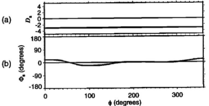
parameters indicate upward propagation in all the frequency range of the AKR. However, the conditions of validity of these estimations may not be fulfilled for the R-X mode. At AKR frequencies the parallel component of the wave electric field cannot be neglected, and the validity of analysis results depends on a relative angle deviation of the antenna from the wave vector. Figure 6 shows simulation results validating the analysis made for the case of November 10, 1996. The simulation has been made for the R-X mode, with all the characteristic frequencies well below (fg -- 23 kHz, f•, = 10 kHz) the selected wave frequency of 150 kHz. The wave vector direction has been defined following the observations at 0 - 145 ø. The simulated waveforms have been corrupted by a broadband Gaussian noise with SNR=3. The results show that the influence of the broadband noise is negligible
10-6 N 3:10-7
(a) • lO_
8
10-9 0.0100 N E 0.0010 (b) "• • o.oool 5 (c) C o -5 1.0 (d)The second example case concerns AKR observations in (e) the HF band of MEMO on November 10, 1996. The spec- trogram in Figure 4 shows intense broadband AKR emis- sions with a low-frequency cutoff varying between 100 and 130 kHz. The waveform measurements of three magnetic
components
and
one
electric
component
give
data
organized
in snapshots of 0.009 s. The most intense signal was ob- served at 1719:45 UT, when the satellite was at invariant lat- itude of 71.2 ø, at 0318 MLT, and at an altitude of 19,182 km.
(•) A detailed analysis of the corresponding snapshot is pre- sented in Figure 5. The AKR emission is seen in the interval from 137 kHz to • 162 kHz, just between two disturbing in- terference signals appearing in the magnetic field data. The
0.5 0.0 • 15o E lOO '"" 50 0 5 180 90 o -90 -180 100 120 140 160 frequency (kHz)
polarization
analysis
of the
wave
magnetic
field
reveals
that Figure
5. Analysis
in the
frequency
interval
100- 170
kHz
in all the frequency range, we observe right-hand nearly cir-cularly polarized waves with a high polarization degree. The waves thus propagate in the R-X mode, and the plane wave approximation may be used. Figure 5e shows that the wave vector is inclined by 30 ø- 40 ø from Bo, but the method of Means [1972] does not give any indication on whether we observe down-going or up-coming waves.
This is provided by parameters Da (Figure 5f) and •a (Figure 5g), which take into account the electric signal. Both
in the HF band. Data were recorded on November 10, 1996, from 1719:45 UT. (a) Sum of the three magnetic autopower spectra; vertical lines and asterisks mark interference sig- nals. (b) Autopower spectrum of the electric component. (c) Sense of polarization in the plane perpendicular to Bo from (4). (d) Degree of polarization from (5). (e) Deviation 0 of the wave vector direction from the ambient magnetic field Bo by the method of Means [ 1972]. (f) Estimate of the
parallel
component
of the Poynting
vector
normalized
by its
13,198 SANTOL•K ET AL.' WAVE-VECTOR DIRECTIONS IN THE NIGHTSIDE AURORAL ZONE 4i 2•
(a)
-4• 180 o• 90 (b) • o • -9o -180 0 1 O0 200 300 q• (degrees)Figure 6. Analysis at 150 kHz as a function of angle az- imuth qb of a simulated R-X mode wave. (a) Estimate of the
parallel
component
of the Poynting
vector
normalized
by its
standard deviation from equation 7. (b) Phase shift between the electric signal and the perpendicular magnetic compo- nent from equation 6. The results are averaged from 100 independent realizations of the data with SNR=3.
and that both the (I'd and Da parameters well reproduce the hemisphere of propagation.
4. Discussion
Analysis of the ELF case of November 12, 1996, shows high inclinations of the Poynting vector from Bo. This ap- parently disagrees with the theory. We have shown that in this particular experimental situation, the results may be ex- plained by the influence of the background noise on the re- sults. The problem may however be also connected to the plasma model that we use for theoretical calculations. First, we must assume a value for the unknown plasma frequency. In a plasma of low density, the value of the plasma frequency may substantially influence whistler mode propagation and the Poynting vector may be found at large angles from Bo. This is possible when the wave frequency becomes lower than the local lower hybrid frequency fth. However, given the measured gyrofrequency value, fth cannot be higher than 555 Hz in an infinitely dense plasma. Therefore the fre- quency band of the observed emission always is above whatever is the plasma frequency. The explanation given in
tion of the bursts of ELF waves, we observe maximum elec-
tron fluxes around 1 keV, and at lower latitudes, the electron
energies increase up to 3-4 keV. We also observe some frac- tion of electrons at energies around 200 eV.
However, there is no clear modulation of the electron en-
ergy spectra connected to pitch angle, and we have no direct evidence for field-aligned beams. Even if we do not find unstable electron distribution functions, it is not in contra- diction with the generation mechanism that we propose. We observe electromagnetic waves that propagate from a dis- tant region above the satellite, and free energy of the un- stable source population has probably been already dissi- pated into the waves. The emissions are very bursty, and we cannot suppose a quasi-static equilibrium which could conserve some features of the original distribution function. The electrons we observe may however have similar ener- gies as the source population. For 4-keV, 1-keV, and 200 eV field-aligned electrons, the Landau resonance condition is satisfied for waves with parallel refractive indices of 8,
16, and 36, respectively. These values may be reached near the whistler mode resonance cone. Indeed, such generation mechanism has been reported by Ergun et al. [1993] who observed enhanced short-wavelength VLF emissions occur- ring during dispersive bursts of low-energy electron fluxes. The measurements were made in the auroral ionosphere, and
electrostatic waves were observed on the whistler mode res-
onance cone with a parallel refractive index of 17. Under
these conditions, unstable features have been identified in
the electron distribution function.
It is widely thought that AKR originates from the rela- tivistic gyroresonant interaction with loss cone distribution of upgoing electrons, as proposed by Wu and Lee [1979]. According to this model, we will suppose generation at fre- quencies around the local electron gyrofrequency. The lower cutoff of intense emission of AKR corresponds then to the highest source altitude. As this cutoff is found at 137 kHz (see Figure 5) and the local electron gyrofrequency is only
23 kHz, the source must be confined well below the obser-
section 3 1 seems then to be the only possible one in the
frame
of
the
line•
theory
of
cold
plasma.
•is theory
also
predicts
a
whistler
mode
refractive
index
which
is
very
ne•
to the experimentally obtained values.
Whistler-mode
auroral
hiss
observed
at
high
altitudes
is
often
considered
to
be
generated
by
the
Landau
resonance
with
auroral
elec•on
beams
[Gurnett
et al., 1983]
In our
'
case,
the
presence
of
the
res
on
an
ce
cone
and
the
observed
high 0 values indicate a simil• generation mechanism. As P'"'
the waves propagate downward, they may be generated by •600 •0 •2o •oao •4o UT a resonant interaction with a beam of down-going electrons.
In Figure
7, simultaneously
recorded
data
of the
ION p•- Fibre 7. (top)
Energy
spec•ogram
of elec•ons
between
ticle
analyzer
[Sauvaud
et al. 1998]
show
elec•ons
at en- 60 eV and
20 keV
detected
by the
ION experiment
on
' November 12, 1996, as a function of UT Shading indicates
ergies
of several
keV.
These
electrons
probably
originate
in the
count
rate
between
0 and
1000
counts
s
-•. (bottom)
the
plasma
sheet,
and
their
energy
gradually
increases
as
the Pitch
angle
of analyzed
elec•ons.
•e vertical
dashed
line
satellite
moves
towed lower
magnetic
latitudes,
from
70.9
ø shows
the position
of the bursty
ELF emissions
observed
by
SANTOL•K ET AL.: WAVE-VECTOR DIRECTIONS IN THE NIGHTSIDE AURORAL ZONE 13,199 INTERBALL-2
iNL:
30o
,;71;
'-l-x• -
,,'
?'
- ," -l, 5-
Y
....
,
x
_1_ _1__ _ I---20•22
•0 • 2
• 4
• 6
•8
•
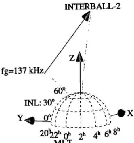
ML•Figure 8. Projection of the wave vector direction of AKR back to the source region. Axes X, Y, and g of the solar magnetic (SM) coordinate system are indicated by arrows. The Earth's surface is marked by parallels at constant invari- ant latitude (INL) and by meridians at constant magnetic lo- cal time (MLT). The wave vector is given by an arrow point- ing toward the satellite position (tip of the arrow, marked INTERBALL-2). The other side of the arrow indicates a place where the local fg reaches 137 kHz. The correspond- ing magnetic lines of force passing through the satellite po- sition and through the possible source region are plotted by dotted lines.
vation point at an altitude of 19,182 km. We thus expect to observe upward propagation in the entire frequency range. This is really confirmed by propagation analysis in Figure 5. Other results of our analysis show that AKR propagates in the R-X mode as a plane wave inclined by 140 ø- 150 ø from
the Earth's magnetic field. The azimuth •b is found between
70 ø and 100 ø (not shown in Figure 5), indicating propaga- tion from lower MLT and lower latitudes. Figure 8 shows a projection of the wave vector back toward the source region. We suppose a negligible refraction, and we follow the direc- tion opposite to the average wave vector direction between
137 and 162 kHz (0 = 146 ø, •b = 86ø). As we go down in altitude and invariant latitude, the electron gyrofrequency in- creases, and on auroral filed lines, it falls into the frequency
interval of the observed AKR emission. The lower cutoff
frequency at 137 kHz becomes equal to the local gyrofre-
quency at an altitude of 7750 km, invariant latitude of 51.1 ø,
and on 2204 MLT. Footprint of the corresponding field line
on the Earth's surface is at invariant latitude of 62.1 ø and on
2231 MLT. Note that we use a simple dipolar model of the magnetic field in this example. Note also that the position of the estimated source region is highly sensitive to the initial 0 value. If we for example use the method of McPherron et al. [1972] instead of the method of Means [1972], we obtain an average 0 of 151 ø, and the above condition for the cutoff frequency is reached at a higher altitude and in- variant latitude, and on a slightly different MLT (8120 km, 63 ø, and 2229 MLT, respectively). These values move the corresponding field line footprint up to an invariant latitude
of 69.7 ø, and to 2258 MLT. A detailed examination of this
problem is beyond the scope of the present paper. How- ever, all these results are roughly consistent with previous findings on AKR propagation known from DE-1 and Viking data [e.g., Gurnett et al., 1983; Calvert and Hashimoto, 1990; Le Qudau and Louarn, 1996]. After WDF analysis of MEMO data by Parrot et al. [2001], our results represent the first direct determination of the complete wave vector direc- tion at AKR frequencies. We use here completely indepen- dent plane-wave methods, and the fact that we may confirm previously obtained results shows the potential of the above presented techniques for future analyses.
5. Conclusions
1. We have described several methods for wave propaga- tion analysis based on simultaneous measurement of several field components. Under some conditions we can determine the complete wave vector direction from three magnetic field components and a single electric field component. With three magnetic and two electric components we can char- acterize the complete wave vector direction, wave refractive index, and the transfer function of the antenna-plasma in- terface. Moreover, the missing electric component may be estimated, and the Poynting vector can be determined.
2. The above analysis techniques can be used to describe wave fields which are near to a single plane wave in a single wave mode. If any of these conditions is violated, the results must be verified by the WDF methods.
3. Application to multicomponent waveform data mea- sured by the MEMO device onboard INTERBALL-2 in the nightside auroral region shows that whistler mode bursty ELF emission observed on November 12, 1996, propagates in the whistler mode at wave vector directions near to the Gendrin angle and not far from the resonance cone. The waves propagate from the nightside sector toward the Earth, in the direction of growing magnetic latitude. Their source must then be at auroral latitudes above 18,300 km. The gen- eration mechanism is probably connected with plasma sheet electrons which are observed at the same time as the ELF bursts.
4. As the second example, we analyse R-X mode AKR
emission observed on November 10, 1996. The results show
that the waves are upgoing with wave vector directions in- clined by 140 ø- 150 ø from Bo, consistently with their gen- eration near the local electron gyrofrequency in the auroral region. After the paper of Parrot et al. [2001], where the
WDF methods have been used, this is the first similar verifi-
cation done by plane wave methods directly from the electric and magnetic waveform data. Both these examples demon- strate a great potential of such kind of analysis for future
applications.
Appendix A: Estimation of the Full Electric
Field Vector Using the Magnetic Field Vector
Data and Two Electric Signals
The Faraday's law in the frequency domain may be used to reconstruct the electric field vector from the magnetic