Validation against sodium loop experimentsof corrosion product contamination code oscar-na

HAL Id: hal-02419683

https://hal.archives-ouvertes.fr/hal-02419683

Submitted on 19 Dec 2019

HAL is a multi-disciplinary open access archive for the deposit and dissemination of sci-entific research documents, whether they are pub-lished or not. The documents may come from teaching and research institutions in France or abroad, or from public or private research centers.

L’archive ouverte pluridisciplinaire HAL, est destinée au dépôt et à la diffusion de documents scientifiques de niveau recherche, publiés ou non, émanant des établissements d’enseignement et de recherche français ou étrangers, des laboratoires publics ou privés.

product contamination code oscar-na

Jb. Genin, L. Brissonneau

To cite this version:

Jb. Genin, L. Brissonneau. Validation against sodium loop experimentsof corrosion product con-tamination code oscar-na. International Conference on Fast Reactors and Related Fuel Cycles Next Generation Nuclear Systems for Sustainable Development (FR17), Jun 2017, Yekaterinburg, Russia. �hal-02419683�

Validation Against Sodium Loop Experiments

of Corrosion Product Contamination Code OSCAR-Na

J.B. Génin1, L. Brissonneau1

1

CEA, DEN, Cadarache, DTN, F-13108 Saint-Paul-Lez-Durance, France

E-mail contact of main author: jean-baptiste.genin@cea.fr

Abstract. The OSCAR-Na code has been developed to calculate the mass transfer of corrosion products and related contamination in the primary circuit of sodium fast reactors (SFR). Indeed, even if fuel cladding corrosion appears to be very limited, the contamination of the reactor components plays an important role in defining the design, the maintenance and the decommissioning operations for SFR.

The modeling is based on the solution/precipitation of the different elements of the steel. These elements dissolve mainly at the hot surfaces, and precipitate on the cold surfaces, and then induce the shifting of the metal/sodium interface (bulk corrosion or bulk deposit). The diffusion in the steel is also taken into account and allows calculating the preferential release of the most soluble elements (nickel, chromium, and manganese). The code uses a numerical method for solving the diffusion equation in the steel and the complete mass balance in sodium for all elements, allowing the calculation of the metal/sodium interface shifting and of the flux of each element through this interface.

Code validation has already been carried out against PHENIX contamination on heat exchanger surfaces for the main radionuclides. This paper presents the continuation of the validation process against experimental results obtained on the STCL sodium loop, with well controlled experimental conditions. Different parameters of the model are adjusted to match concentration profiles in the metal and elementary releases measured at 604 °C. These parameters are the solubility in the sodium and the diffusion coefficient in the steel for each element, as well as the oxygen-enhanced iron dissolution rate. The new values are compared to those published in the literature and discussed. Moreover the modeling allows reproducing the effects of oxygen concentration, and sodium velocity which were varied in the experiments.

Key Words: Corrosion, OSCAR-Na, Sodium loop, Contamination

1 INTRODUCTION

The OSCAR-Na code has been developed to calculate the mass transfer of corrosion products and related contamination in the primary circuit of sodium fast reactors (SFR). The modeling assumes that the transfer between steel and sodium is primarily by solution and precipitation of metallic elements, rather than by particle detachment and particle deposition.

The code has already been validated against 54Mn, 58Co and 60Co contamination in the intermediate heat exchangers (IHX) of the French PHENIX reactor [1]. This validation process has allowed adjusting parameters (mainly diffusion coefficient in the metal and equilibrium concentration in the sodium) regarding manganese and cobalt elements, as well as iron which dissolution or precipitation governs the metal/sodium interface shifting.

In this paper, code validation is continued against experiments in the STCL sodium loop (HEDL, Westinghouse, operated in the 1970’s). Individual mass losses of alloy elements as well as composition profiles were carefully measured on irradiated 316 stainless steel specimens by Brehm and coworkers [2,3,4], using electropolishing and atomic absorption

spectroscopy or radiochemical analysis. Experiments were performed for different temperatures, oxygen contents in the sodium, sodium velocities and durations of exposure to sodium. The goal here is to verify that the OSCAR-Na modeling allows reproducing the experimental releases for the different conditions, and to adjust the model parameters for the different alloy elements, mainly nickel and chromium.

After a reminder of the code modeling (§ 2) and a description of the experimental results (§ 3), comparison between simulation and measurements is presented (§ 4), and adjusted parameters are compared to published values and discussed (§ 5).

2 THE OSCAR-Na CODE

2.1 Basics

The OSCAR-Na code is based on the OSCAR code [5], a mass transfer code dedicated to pressurized water reactors. Fluid systems are discretized into as many volumes or regions as necessary. These regions are defined by geometric, thermo hydraulic, neutron flux, material properties, and operating characteristics. Then for each region and each isotope considered, a mass balance is calculated in the sodium and in the metal. The considered mechanisms are the solution/precipitation model (cf. § 2.2) which generates mass transfers between metal and sodium, as well as the convection, which transports species throughout the primary circuit. It includes the purification system (cold trap), this latter removing species from the circuit with a given efficiency. Moreover, the nuclides are described within filiation chains, taking into account radioactive decay constant and capture cross section if necessary.

2.2 The transfer model at the metal/sodium interface

A solution/precipitation model is considered at the steel/sodium interface, based on mass transfer theory [1,6]. The mass flux Φ between sodium and steel is obtained by equating the fluxes at both sides of the interface:

      − ⋅ = ⋅ + ∂ ∂ ⋅ = Φ = ' 0 C C K C u x C D eff i i x

β

(1) where C and C’ are the nuclide concentration (g/m3) in the steel and bulk sodium, respectively (the subscript i indicating interfacial values at x = 0). In OSCAR-Na, C’ is calculated through a complete mass balance around the primary circuit, and C is obtained by numerical _i solving of the general diffusion equation in the steel:

R C x C u x C D t C + ⋅ − ∂ ∂ ⋅ +       ∂ ∂ ⋅ = ∂ ∂

_λ

2 2 (2)

with eq. (1) as boundary condition at the interface (

λ

is the decay constant of the considered radionuclide, and R is the rate of production by neutron activation).

Thus, the main parameters of the model are, for each element:

• D (m2/s): diffusion coefficient in the austenitic stainless steel. A higher diffusion coefficient can also be considered in the ferrite layer which forms near the steel surface due to nickel depletion.

• eff

K (m/s): effective mass transfer coefficient between interface and bulk sodium. It corresponds to the limiting value between the diffusion rate through the sodium

laminar boundary layer (k) and the dissolution or precipitation rate (k ) at the _a interface: a a eff k k k k K + ⋅ = .

• β: dimensionless chemical partition coefficient. It is related to the concentration C' éq in the sodium at equilibrium with the steel surface by C'_éq=C_i β. For a pure element, β varies inversely with respect to the solubility.

• u (m/s) is the interfacial velocity or moving rate of the sodium/steel interface, due to dissolution and precipitation. It is positive or negative in case of bulk corrosion (dissolution) or bulk deposition (precipitation) respectively.

In OSCAR-Na, additional assumptions are taken into account:

• For other elements than iron, it is considered that the surface reaction rate ka is much greater than the diffusion rate k through the sodium boundary layer: Keff =k (local chemical equilibrium is obtained at the steel/sodium interface for these elements).

• For iron, the surface reaction involves oxygen which acts as a catalyst. Then the iron solution/precipitation kinetic k_a,Fe depends on oxygen content in the sodium

[ ]

O , following a relationship of the type:

[ ]

RT

E n Fe a Fe a k O e k _, = 0_, ⋅ ⋅ − ⋅ [7].

• For all elements, the mass transfer coefficient k through the boundary layer in the flowing sodium is calculated from the following equation:

h Na d D Sc k = ⋅ 0.8⋅ 13 ⋅ Re 023 .

0 [8], where Re and Sc represent the Reynolds and Schmidt numbers, respectively, D_Na is the diffusivity of the element in liquid sodium, and d the equivalent hydrodynamic diameter of the flow path. _h

• The iron concentration profile in the steel is assumed to be uniform. Consequently, the iron flux at the interface is stoichiometric: Φ_Fe =u⋅C_Fe, and the interfacial velocity is governed by iron behavior (see eq. (1)):

        − ⋅ = Fe éq Fe Fe eff Fe C C K u , ' ' 1 β (3)

Lastly, integration of the diffusion equation (2) for stable elements gives the following expression for mass loss (or gain) for each element (g/m2):

(

)

∫

∫

∫

₀Φ(t')⋅dt'= ₀C∞ ⋅u(t')⋅dt'+ ₀∞ C∞ −C(x,t) ⋅dx t t (4)

where C is the element concentration in the steel far from the surface. _∞

The first right hand term is the stoichiometric contribution to mass loss (or gain): alloy elements are removed with the iron, as iron is the major element of the steel structure. The second term is the preferential release contribution. In hot regions where bulk corrosion occurs, the preferential release (or leaching) is effective for elements with large solubility in sodium (Ni, Cr, Mn). The steel surface is locally depleted in these elements. When the nickel concentration is low enough, a layer of ferrite is formed on the surface of the steel in which higher diffusivity is considered. Conversely, less soluble elements (Mo, Co) are retained in the metal, which leads to enrichment in these elements near the surface.

2.3 STCL loop description

The specimens used for studies in the Source Term Control Loop (STCL) [2,3,4] were sections cut from fuel cladding tubes irradiated at 370 °C in a fast reactor.

For OSCAR-Na simulation, the STCL circuit is discretized in around 30 regions to represent the temperature variation along the circuit. The key points taken into account in the code data set are the following:

• Typical specimen composition (as well as for the loop pipes):

65% Fe, 17% Cr, 13% Ni, 2.5% Mo and 1.5% Mn (AISI 316 stainless steel). • Specimen temperature: 604 °C

• Main loop minimum temperature: 427 °C • Sodium velocity at the specimens: 6.7 m/s • Primary flow rate: 0.1 kg/s

• Reynolds number at the specimen interface: 4.4 104

• Oxygen levels in the sodium have been evaluated by Brehm at al. to 0.5 and 2.5 ppm from the cold trap temperature (115 °C and 154 °C respectively)

• Flow rate on cold trap: 10% of main flow. Cold traps are considered as fully efficient for alloy element trapping.

3 EXPERIMENTAL RESULTS OBTAINED IN STCL LOOP

3.1 Composition profiles and element mass losses

A technique was developed by HEDL [2] to remove successive layers from the surface of the radioactive specimen by electropolishing, followed by atomic absorption spectroscopy and radiochemical analysis of the polishing solution. The depth of increment analyzed can be varied by varying the polishing time. Usual increment depths are 0.2 to 1 µm. Fifteen to twenty increments are usually analyzed to construct composition profiles of elements and radionuclides in the steel after sodium exposure.

Figure 1 : Concentration and radiochemical profiles obtained on irradiated 316 SS exposed for 6000 hours in sodium [2]

Profile examples [2] are given in Fig. 1 for an irradiated 316 stainless steel specimen exposed for 6000 hours in sodium at 604 °C and 2.5 ppm oxygen. This specimen will be designed as the reference specimen further in the paper. The profiles show a depleted zone containing a porous structure and concentration gradients of Ni, Cr, Mn, Mo and Co, and an unaffected region beneath the depleted zone. Close to the interface, a thin layer of ferrite is stable, and is characterized by higher element diffusivity.

Moreover, the weight loss ∆M_elt of each alloy element elt can be calculated from data obtained with this incremental analysis technique [2].Individual weight losses ∆Melt for the reference specimen are given in table 1, as well as the element mass fraction

χ

_elt evaluated from deep layer analysis.

Table 1 – Individual mass losses measured on the reference specimen [3]

A lot of specimens were exposed to sodium in the STCL loop and analyzed according to the incremental analysis technique. Therefore linear functional correlations of mass loss versus time are proposed by Brehm for each alloy element [3,4], for different temperatures (538 °C and 604 °C) and different oxygen levels (0.5 ppm and 2.5 ppm).

3.2 Assessment of stoichiometric and preferential releases

Brehm measured similar iron masses in the different layers [2]. Assuming that the depths of the incremental layers are similar, this shows that the iron concentration profile in the steel is uniform, which is in accordance with the assumption done in OSCAR-Na modeling (cf. § 2.2). Then iron release is stoichiometric and the stoichiometric and preferential contributions to experimental mass losses can be obtained for each element as follows:

• Fe elt Fe stoechio elt M M =∆ ⋅

χ

_χ

∆ • stoechio elt elt préf elt M M M =∆ −∆ ∆ .

Stoichiometric and preferential mass losses for the reference specimen are given in table 1.

4 SIMULATION WITH OSCAR-Na

In this paper, we try to reproduce with the OSCAR-Na code the individual mass losses measured at 604 °C, and oxygen levels of 0.5 ppm and 2.5 ppm. First, model parameters are adjusted to match mass losses measured for each element on the reference specimen (6000 hours, 2.5 ppm oxygen), for which detailed data allowing profile construction are published [2]. Then calculated mass losses are compared with experimental linear correlations versus time at 604 °C and 2.5 ppm oxygen. Lastly, oxygen-enhanced iron dissolution rate k_a,_Fe is adjusted to match experimental mass losses at 0.5 ppm oxygen.

Mass fraction χelt Total mass loss ∆Melt (g/m 2 ) Stoichiometric mass loss (g/m2) Preferentiel mass loss (g/m2) Fe 67.9% 7.5 7.5 0.0 Ni 12.3% 4.2 1.4 2.8 Cr 16.0% 4.4 1.8 2.6 Mn 1.3% 0.5 0.1 0.4 Mo 2.5% 0.4 0.3 0.1 Total 100.00% 17.0 11.1 5.9

4.1 Stoichiometric release adjustment for reference specimen

As iron release is stoichiometric (ΦFe =CFe⋅u), then its measurement is equivalent to that of the interfacial velocity 1 (1 ' )

, , , Fe éq Fe Fe a Fe Fe a Fe Fe C C k k k k u ⋅ − + ⋅ ⋅ =

β (see eq. (3)). In this equation, two parameters are not well known (cf. § 5): k_a,Fe and

β

Fe. Iron release increases with iron equilibrium concentration (related to

β

_Fe) and iron dissolution rate (k_a,_Fe), and then its measurement is not sufficient to adjust both parameters.

An experimental study of iron release versus sodium velocity would allow distinguishing both parameters k_a,_Fe and

β

Fe. Indeed, diffusion rate kFe through the sodium boundary layer varies like sodium velocity at the power 0.8. Then iron release strongly increases with sodium velocity as long as k_Fe <k_a,_Fe, and becomes slightly dependent on sodium velocity when the latter is greater than a critical velocity defined by kFe =ka,Fe. This critical velocity is independent of iron equilibrium concentration, and its experimental assessment allows evaluating ka,Fe if kFe is a known function of sodium velocity.

Such experimental studies were carried out by different authors [9], although they concern total release (for all elements) versus sodium velocity. The critical sodium velocity can then be assessed only if stoichiometric release is predominant over the preferential release, i.e. if oxygen content in the sodium is high enough (cf. § 4.5).

In this paper, the

β

_Fe parameter at 604 °C has been chosen in order to obtain critical velocities consistent with literature typical values [9], even if they have been obtained at higher temperature and higher oxygen content than in the STCL loop. Indeed, if

β

Fe value is fixed, OSCAR-Na simulation allows adjusting k_a,_Fe to match iron release measurement in the STCL loop at 6.7 m/s sodium velocity and this determines the critical velocity. Moreover this latter depends on oxygen content like ka,Fe. Thus, from the chosen value for

β

Fe (independent of oxygen content) and from the iron release measurement at 0.5 ppm and 2.5 ppm, critical sodium velocity at 604 °C in the STCL loop is evaluated to 0.07 m/s and 2.1 m/s respectively. Iron solubility deduced from the

β

_Fe value will be compared to literature data in § 5.

4.2 Reconstruction of concentration profiles

As well as for the stoichiometric release, the simulated preferential release for each element must be adjusted to match the measured mass loss. However the preferential release of an element depends mainly on its diffusivity in the steel and equilibrium concentration in the sodium, and both parameters cannot be distinguished if only the preferential mass loss is known.

Fortunately, detailed data are available [2] for the reference specimen. These data allow evaluating the preferential mass loss from the concentration profiles (see eq. (4)):

(

)

∫

∞ ∞ − ⋅ = ∆ 0 ( , ) ) (t C C x t dx Mpref (g/m 2 )

Nevertheless, concentration profiles presented in Figure 1 have been recalculated to take into account OSCAR-Na modeling. Indeed, Brehm et al. evaluated the depth µ of an

incremental layer from the layer mass m measured by atomic absorption spectroscopy, as _tot well as the steel density

ρ

_steel and the specimen area S:

µ

_Brehm =m_tot

(

ρ

_steel ⋅S

)

. But in the depleted zone, the measured layer mass is lower than the initial mass, which induces underestimation of the layer depths as calculated by Brehm.

Assuming that iron concentration profile is uniform (cf. § 3.2), layer depths have been reevaluated from measured iron mass in the layer m and iron volume concentration in the _Fe steel C_Fe:

µ

_OSCAR−Na =m_Fe

(

C_Fe⋅S

)

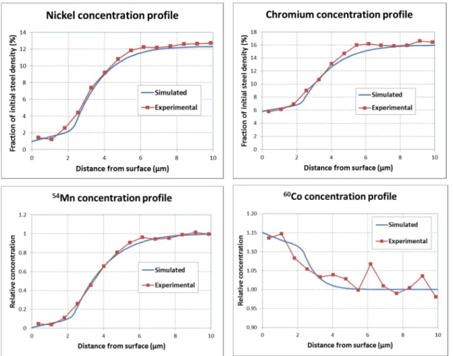
. Moreover, profile abscissa has been modified to correspond to the distance to the interface of the middle of the layer rather than the edge of the layer.

The recalculated experimental concentration profiles are plotted in Figure 2 for nickel and chromium, as well as for 54Mn and 60Co. In addition to abscissa reevaluation, they differ from those in Figure 1 as element volume concentration divided by initial steel density is considered instead of element mass fraction. This provides the same value far from the steel surface, but not in the depleted zone. As for radionuclides, the relative concentration in comparison to the one far from the steel surface is plotted instead of the absolute concentration.

4.3 Preferential release adjustment for reference specimen

The following OSCAR-Na parameters have been adjusted to match the concentration profiles of the reference specimen, and thus the preferential release:

• The chemical partition coefficient β (or equilibrium concentration) for each element, which governs concentration at the interface. The adjusted values will be discussed in § 5.

• The diffusivity in the steel for each element, which governs the depth of the depleted zone.

• The nickel concentration beneath which austenite turns into ferrite. The adjusted value is 2% of steel density.

• The increase factor of diffusivity in the ferrite layer compared to the austenite. The adjusted factor is 10, which is consistent with Brissonneau’s results [7].

Figure 2 shows that experimental profile concentrations for nickel, chromium, 54Mn, and 60Co can be correctly simulated by adjusting the above parameters.

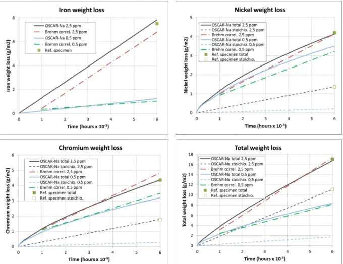
It is worth noticing that the simulated preferential release perfectly matches experimental mass losses given in table 1 for each element. This is illustrated in Figure 3 where the stoichiometric and total mass losses measured for the reference specimen are represented by the marks at 6000 hours. This model calibration could not have been achieved without the concentration profile data, as the different parameters could not have been assessed separately.

Furthermore, the agreement between concentration profile and derived preferential mass loss is actually independent of OSCAR-Na modeling as it could be achieved by simply integrating the experimental concentration profiles. This validates the method used for profile construction (cf. § 4.2), and confirms the uniform profile assumption for iron which was necessary to obtain this agreement.

Figure 2 – Experimental and simulated concentration profiles for the reference specimen

4.4 Simulation of individual mass losses at 2.5 ppm oxygen

Adjusted parameters on the reference specimen have been retained to simulate individual mass losses versus time at 604 °C and 2.5 ppm oxygen. Comparison with linear functional correlation proposed by Brehm is shown in Figure 3. A good agreement is observed for each element and for total mass loss, which validates the parameters at 604 °C and 2.5 ppm oxygen.

4.5 Simulation of individual mass losses at 0.5 ppm oxygen

The only oxygen dependent model parameter is the iron dissolution rate k_a,Fe. It has been lowered by a factor 15 to simulate the decrease by a factor of around 7 of the iron mass loss at 0.5 ppm compared to 2.5 ppm oxygen. Simulated mass losses for each element are then compared to Brehm linear correlations in Figure 3 and a good agreement is still observed. This shows that OSCAR-Na modeling can well reproduce the effect of oxygen content in the sodium on alloy element corrosion. As the ratio between both oxygen contents is 5, the oxygen content exponent in the iron dissolution rate dependency can be assessed at 1.68. In addition, it may be observed in Figure 3 that preferential mass loss (difference between total and stoichiometric mass losses) is only slightly affected by oxygen content drop. It is consistent with the fact that if interfacial velocity is low enough, preferential and stoichiometric contributions to mass loss can be evaluated separately, with no coupling between both mechanisms [10]. A lower iron dissolution rate has then little impact on the preferential release of nickel and chromium.

Figure 3 – Experimental and simulated individual mass losses at 604 °C, 0.5 and 2.5 ppm oxygen

4.6 Effect of sodium velocity

A leakage of sodium around a regenerative heat exchanger tube-to-shell junction in STCL diverted the sodium flow from the test section, causing the sodium velocity near the specimens to drop under 1 m/s. The test parameters were 604 °C hot leg temperature, 0.1 to 0.3 ppm oxygen in the sodium, and 2450 hours test time. Brehm et al. compared the data obtained in this low velocity test with those in the usual high velocity corrosion tests at 0.5 ppm oxygen. It appears that the material release rates are much lower at the low velocity. This is especially true for the total weight loss, which is a factor of 15 lower at the low velocity, whereas the 54Mn release decreased only by a factor of 4 [4].

In Figure 4 are plotted the experimental 54Mn, Ni and Cr concentration profiles at the low and high sodium velocities, after 2450 hours and 3000 hours of sodium exposure respectively. The depletion near the surface is obviously much smaller at the low velocity, which accounts for the observed difference in material release.

Moreover, Brehm et al [4] noticed that “the depletion of Ni and Cr not only leads to a ferrite layer formation near the surface, but also excess vacancies within the austenite adjacent to the ferrite layer. Although austenite vacancies and ferrite layer formation occur at the low velocity, the thickness of ferrite layer and the number of vacancies in austenite are considerably smaller at the low velocity. This can account for enhanced 54Mn diffusivity at the high velocity, resulting in the observed greater 54Mn release”. Brehm et al. evaluated from

54

Mn depleted zone thickness that the diffusivities of 54Mn in the specimens at the two velocities differ by a factor of 10.

Figure 4 – Experimental concentration profiles at low and high sodium velocity (604 °C, 0.5 ppm oxygen) [4]

OSCAR-Na calculations have been performed to simulate the effect of sodium velocity. A by-pass in the regenerative heat exchanger is introduced in the STCL loop modeling, and flow rate as well as sodium velocity are reduced near the specimens. Adjusted parameters at 0.5 ppm oxygen are retained (cf. § 4.5) but diffusivity in the steel is reduced by a factor of 10 for all alloy elements to take into account the lower amount of vacancies for bulk diffusion. Figure 5 shows calculated concentration profiles at 0.5 ppm oxygen in the following conditions:

• Low diffusivity in the steel, 2450 hours in sodium, 0.01 / 0.2 / 6.7 m/s sodium velocity • High diffusivity in the steel, 3000 hours in sodium, 6.7 m/s sodium velocity

Figure 5 – Simulated concentration profiles at low and high sodium velocities (604 °C, 0.5 ppm oxygen)

It can be observed, by comparing Figures 4 and 5, that 54Mn simulated profile at 0.2 m/s sodium velocity is consistent with the experimental profile, which is due to taking into account low diffusivity rather than low sodium velocity. Indeed, it is the diffusivity in the steel that governs the depth of the depleted zone. It is also in accordance with the 54Mn release reduction of a factor 4 at low velocity.

As for nickel (and chromium), the quasi uniform experimental profile is not reproduced, even with very low sodium velocity (0.01 m/s). Iron behavior does not play any role in this result as interfacial velocity is low enough so that there is no coupling between stoichiometric and preferential releases (cf. § 4.5).

Analysis of the solution/precipitation model integrated in OSCAR-Na shows that if sodium concentration is much lower than equilibrium concentration, element concentration at the interface primarily varies inversely with respect to k β value, i.e. to diffusion through the sodium boundary layer and to equilibrium concentration. Moreover, the lowest the k β value is, the strongest this inverse dependency is. Then as manganese equilibrium concentration is higher compared to nickel or chromium, it induces a lower dependence of

54

Mn profile on sodium velocity. As for nickel and chromium, it seems that the k β value is too high in the simulation. A lower equilibrium concentration for nickel and chromium would improve the simulation but is not compatible with experimental concentration profiles obtained on the reference specimen at 6.7 m/s sodium velocity. A higher sodium velocity exponent in the k expression could also improve the simulation.

However limited data available on the low velocity test conditions and experimental results preclude further analysis. At least, enhanced 54Mn diffusivity due to nickel and chromium depletion is confirmed by the low velocity test simulation, as well as a higher manganese equilibrium concentration compared to nickel and chromium. Element diffusivity in 316 SS in OSCAR-Na modeling should then be related to subsurface depletion leading to enhanced vacancy concentrations.

5 DISCUSSION

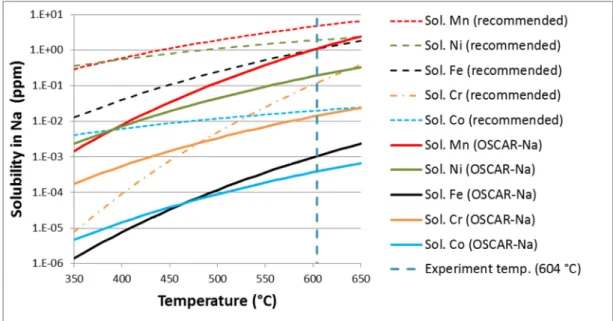
Pure element solubility in the sodium can be assessed from the element chemical partition coefficient β used in the OSCAR-Na code, assuming that activity coefficient of element in steel is equal to 1. Code solubilities thus obtained are compared in Figure 6 to published recommended values [11], which were measured at equilibrium with pure elements.

For other elements than iron, the β parameter has been finely adjusted at 604 °C from STCL experiments as described in this paper. Its temperature dependence has been evaluated from code validation on PHENIX intermediate exchanger contamination and still has to be consolidated for chromium and nickel. We observe in Figure 6 that code solubilities at 604 °C are lower than measured values by around one order of magnitude. For nickel and manganese, a low activity coefficient could account for this difference. For chromium, the formation of metastable ternary oxides with Na could also be an explanation. Indeed, chromium is known to form stable NaCrO2 at slightly higher oxygen contents.

As for iron, the

β

_Fe parameter cannot be determined precisely from STCL experiments (cf. § 4.1). However it has been assessed in accordance with published studies. Moreover, it has long been recognized that the apparent solubility of iron consistent with the results of mass transfer in sodium loop is much lower than the one determined in solubility experiments [8,12]. This is confirmed in our study (cf. Fig. 6), where the solubility value at 604°C (related to

β

_Fe) is three orders of magnitude lower than the current accepted value [11]. This discrepancy cannot be explained by iron activity coefficient in the steel at the surface, as it is very close from pure bcc iron used in the solubility experiments. As proposed in [9], Na-Fe-O interactions could be an explanation.

Nevertheless, limited uncertainty remains on iron equilibrium concentration: it could be up to 10 times higher than the value chosen in this paper. It directly impacts the assessment of the iron dissolution rate k_a,_Fe and its oxygen dependency. Indeed, if a higher iron equilibrium concentration was retained, k_a,_Fe and then the critical velocity would be lower (cf. § 4.1). The interfacial velocity u would tend towards

Fe Fe a k u

β

,

lim = if iron concentration in the sodium is much lower than equilibrium concentration and the iron dissolution rate reduction factor between 2.5 ppm and 0.5 ppm oxygen would tend towards the ratio (around 7) between iron releases at both oxygen contents. The oxygen exponent would then be lower, but still greater than 1. It should be added that the oxygen exponent also depends on the relationship chosen between cold trap temperature and oxygen content evaluation.

6 CONCLUSION

The simulation of tests performed in the STCL loop confirms OSCAR-Na modeling ability to calculate weight losses due to corrosion of 316 SS in sodium circuits. Especially detailed published data enabled a fine adjustment of the main model parameters at 604 °C, mainly the equilibrium concentration in sodium and the diffusivity in steel, for each element except iron. For iron, limited uncertainty remains on equilibrium concentration and the latter must be jointly adjusted with iron dissolution rate. Furthermore, the impact of oxygen is well reproduced by taking into account the oxygen-enhanced iron dissolution rate, provided the oxygen dependency coefficient is adjusted. Enhanced diffusivity due to nickel and chromium depletion in steel subsurface (increasing vacancy concentration) has also been highlighted. The code validation must be pursued on reactor contamination and sodium loop experiments in order to define the dependence of the model parameters with temperature, and to assess more precisely the iron equilibrium concentration in SFR primary sodium conditions. Moreover, based on the present findings, element diffusivity in 316 SS in OSCAR-Na modeling will have to be made dependent on nickel and chromium depletion.

Références

[1] J.-B. Génin et al., “OSCAR-Na V1.3: a new code for simulating corrosion product contamination in SFR”, Metallurgical and Material Transactions E, pp 291-298, Volume 3E, December 2016

[2] W.F. Brehm et al., “Techniques for Studying Corrosion and Deposition of Radioactive Materials in Sodium Loops”, IAEA Specialists Meeting on Fission and Corrosion Product Behaviour in Primary Systems of LMFBR’s, Dimitrovgrad USSR, 1975

[3] W.F. Brehm, “Effect of Oxygen in Sodium upon Radionuclide Release from Austenitic Stainless Steel”, IAEA Specialists Meeting on Fission and Corrosion Product Behaviour in Primary Systems of LMFBR’s, Dimitrovgrad USSR, 1975

[4] W.F. Brehm et al., “Corrosion Product Release into Sodium from Austenitic Stainless Steel”, H.U. Borgstedt (Ed.) Material Behavior and Physical Chemistry in Liquid Metal Systems, pp. 193-204, 24-26 mars, 1981

[5] J.-B. Génin et al., “The OSCAR code package : a unique tool for simulating PWR contamination”, Proceeding of the International Conference on Water Chemistry of Nuclear Reactors Systems, NPC, October 2010, Quebec (Canada), 2010.

[6] M.V. Polley and G. Skyrme, “An analysis of radioactive corrosion product transfer in sodium loop systems”, Journal of Nuclear Materials 75 (1978) 226-237

[7] L. Brissonneau, “New considerations on the kinetics of mass transfer in sodium fast reactors: an attempt to consider irradiation effects and low temperature corrosion”, Journal of Nuclear Materials 423 (2012) 67-78

[8] R.E. Treybal, Mass Transfer Operations, Mc Graw-Hill, New York, 1965

[9] J.R. Weeks and H.S. Issacs, “Corrosion and deposition of steels and nickel-base alloys in liquid sodium”, Advances in Corrosion Science and Technology (1973) 3; 1-66 [10] J.W. Anno, J.A. Walowit, Nuclear Technology 10 (1971) 67-75

[11] H.U. Borgstedt, C.K. Mathews, Applied Chemistry of the Alkali Metals, Plenum Press, New York, 1987

[12] C.F. Clement, P. Hawtin, The corrosion of steels in liquid sodium, in: M.H. Cooper (Ed.) International Conference on Liquid Metal Technology in Energy Production, American Nuclear Society, Champion, Pennsylvania, 3-6 may 1976, 1976, pp. 393-399