HAL Id: inria-00533617
https://hal.inria.fr/inria-00533617v2
Submitted on 1 Nov 2011
HAL is a multi-disciplinary open access
archive for the deposit and dissemination of
sci-entific research documents, whether they are
pub-lished or not. The documents may come from
L’archive ouverte pluridisciplinaire HAL, est
destinée au dépôt et à la diffusion de documents
scientifiques de niveau recherche, publiés ou non,
émanant des établissements d’enseignement et de
(Workpackage 1.1)
Françoise Balmas, Alexandre Bergel, Simon Denier, Stéphane Ducasse, Jannik
Laval, Karine Mordal-Manet, Hani Abdeen, Fabrice Bellingard
To cite this version:
Françoise Balmas, Alexandre Bergel, Simon Denier, Stéphane Ducasse, Jannik Laval, et al..
Soft-ware metric for Java and C++ practices (Workpackage 1.1). [Research Report] 2010, pp.44.
�inria-00533617v2�
Référencement des métriques utiles
à la caractérisation des pratiques sensibles
pour Java et C++
Workpackage: 1.1
This deliverable is available as a free download.
Copyright c 2008–2010 by F. Balmas, A. Bergel, S. Denier, S. Ducasse, J. Laval, K. Mordal-Manet, H. Abdeen, F. Bellingard.
The contents of this deliverable are protected under Creative Commons Attribution-Noncommercial-ShareAlike 3.0 Unported license.
You are free:
to Share — to copy, distribute and transmit the work to Remix — to adapt the work
Under the following conditions:
Attribution. You must attribute the work in the manner specified by the author or licensor (but not in any way that suggests that they endorse you or your use of the work).
Noncommercial. You may not use this work for commercial purposes.
Share Alike. If you alter, transform, or build upon this work, you may distribute the resulting work only under the same, similar or a compatible license.
• For any reuse or distribution, you must make clear to others the license terms of this work. The best way to do this is with a link to this web page: creativecommons.org/licenses/by-sa/ 3.0/
• Any of the above conditions can be waived if you get permission from the copyright holder. • Nothing in this license impairs or restricts the author’s moral rights.
Your fair dealing and other rights are in no way affected by the above. This is a human-readable summary of the Legal Code (the full license):
http://creativecommons.org/licenses/by-nc-sa/3.0/legalcode
Workpackage: 1.1
Title: Software metric for Java and C++ practices
Titre: Référencement des métriques utiles à la caractérisation des pratiques sen-sibles pour Java et C++
Version: 2.0
Authors: F. Balmas, A. Bergel, S. Denier, S. Ducasse, J. Laval, K. Mordal-Manet, H. Abdeen, F. Bellingard
Planning
• Delivery Date: 26 January 2009 • First Version: 15 October 2008 • Final Version: 31 March 2010
Contents
1 The Squale Quality Model in a Nutshell 6
2 Metrics Meta Model 8
3 Software Metrics Assessment 10
3.1 Primitive Metrics . . . 10 3.2 Design Metrics . . . 21
3.3 New Metrics and Missing Aspects . . . 34
Rationale and Technological Challenges
Objectives. The objective of this deliverable is to define a catalog of software metrics. In particular we analyze the metrics used in the Squale Model and tool. In addition it offers a coherent set of software metrics for object-oriented languages on top of which Squale practices will be based. There is a plethora of software metrics [LK94, FP96, HS96, HK00, LM06] and a large amount of research articles. Still there is a lack for a serious and practically-oriented evaluation of metrics. Often metrics lacks the property that the software reengineer or quality expert can easily understand the situation summarized by the metrics. In particular since the exact notion of coupling and cohesion is complex, a particular focus on such point is important.
Technological Challenges. Since the goal of the Squale project is to assess the quality of software system, we identify the following challenges for software metrics.
• Validated. • Clearly Defined. • Understandable.
Pertinence and Completeness of Quality Models. The pertinence of a model is based on its capability to model/qualify a lot of complex practices from software metrics (de-sign patterns or poorly structured code for example). The quality is a feature very complex to capture. The second difficulty is to find a model which must be continuous and with no threshold effect: it should avoid for example that cutting of a complex method in 3 other complex methods - but more readable - spoils the result. The third difficulty is to have a model universal and stable enough to allow change application monitoring which can be use to compare similar applications using benchmarking. Fi-nally, like other measures, quality indicators may be manipulated/deviated. The model must be consequently simple to explain and rich enough at the same time to not be deviated easily.
This document describes a selection of current software metrics that will be used in Workpackage 1.3 to define more advanced elements (practices) of the Squale quality model.
Chapter1. The Squale Quality Model in a
Nut-shell
This section presents the main elements of the Squale software quality model as well as their structural relationships. In the following section, we present other quality models and show that they are different from the Squale one.
The quality model implemented in the Squale environment is based on software metrics and their aggregations which we will detail just after and in more detail in Workpackage 1.3. Here we illustrate one of the key aspects of the model and differ-ence between software metrics and practices as defined in the Squale Model. If we take the metric indicating the number of methods covered by tests, we get a software metrics. To be able to qualify this raw metric and to be able to stress that from a quality point of view it is important that complex methods are covered and that the impact of simple accessor methods is lowered, Squale introduces a practice which combines the previous metric with others such as the McCabe complexity. Hence by abstracting from the immediate software metrics, the Squale model allows the reengineer to stress and provide more meaningful quality oriented perceptions of the software.
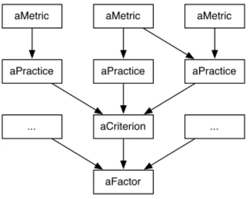
The Squale model is composed of four elements, each having a different granular-ity. Figure 1.1 presents the four levels of the Squale model. Starting from the most fine-grained element, it is an aggregation of metrics, practices, criteria and factors.
aMetric aPractice aCriterion aFactor aMetric aMetric aPractice aPractice ... ...
Figure 1.1: Squale Software Quality Structuring Elements.
• A metric is a measurement directly computed from the program source code. The Squale tool current implementation is based on 17 metrics.
• A practice assesses one quality of a model, from a "white box" technical point of view. A practice is associated to one or more metrics. 50 practices are currently implemented.
• A criterion assesses one principle of software quality, from a "black box" point of view. It averages a set of practices. Such a principle could be safety, simplicity, or modularity. For now, 15 criteria are implemented.
• A factor represents the highest quality assessment, typically for non-technical persons. A factor is computed over a set of averaged criteria. 6 factors are currently available and are explained in a following section.
Chapter2. Metrics Meta Model
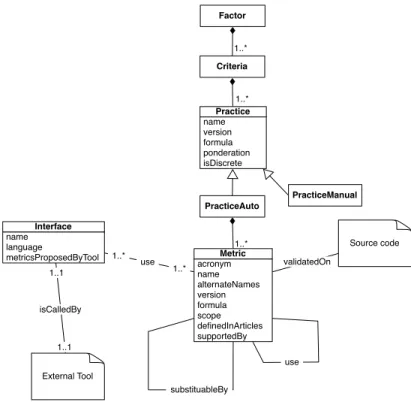
A metric is a measurement on a source code. It is a function that returns a numer-ical value which evaluates a source code. As such, metrics are considered as low level. Literature on metrics provides a significant amount of metrics such as the well known Depth Inheritance Tree (DIT, HNL) and Specialization Index (SIX) [LK94, HS96, Kan02]. Figure 2.1 shows the different informations collected to fully represent a metric. A metric is characterized by:
acronym an acronym to identify the metric.
names a name and a list of alternative names (a metric may have several names). version a version number (the version number refers to possible different
implementa-tions of the same metric). This allows one to have an history of the metric. formula a formula which computes the metric and returns the result of the metric.
scope a scope which declares the entities on which the metric can be computed. references a bibliographic pointing to the articles precisely defining the metrics. This
pro-vides a complete documentation and we can know on which entities the metric is based.
tools a list of tools which support the metric. This allows one to know tools influence and traceability. supportedBy lists the list of tools implementing the metrics. This provides some tools which can be used to compute the metrics. This allows to know tools influence and traceability.
sample a reference sample and its associated result against which the metric can be tested for non-regression. This allows one to evolve the metric with a Validation Code (certification).
alternates possible metrics that could be used to replace the current one. Some metrics compute the same things but differently. This helps substituting a metric by another one in case tools do not support one metric but the other.
required metrics a (possibly empty) list of metrics which are used in the computation of the metric. The output will be a meta-model for metric description.
Example. For the metric Depth of Inheritance Tree: acronym := ’DIT’
name := ’Depth of Inheritance Tree’
alternateNames := #(’Hierarchy Nesting Level’) version := ’1.0’
scope := Class formula: aFamixClass
1..* 1..* Factor Criteria PracticeAuto PracticeManual 1..* Source code External Tool substituableBy name language metricsProposedByTool Interface acronym name alternateNames version formula scope definedInArticles supportedBy Metric name version formula ponderation isDiscrete Practice validatedOn 1..1 1..1 1..* 1..* use isCalledBy use
Figure 2.1: Meta model for metrics.
ˆ aFamixClass superclassHierarchy size definedInArticles := nil
supportedBy := nil substituable := nil use := nil
Chapter3. Software Metrics Assessment
3.1
Primitive Metrics
Primitive metrics target some basic aspects of source code entities (DIT, NOM), or a simple combination of other primitives (WMC, SIX) to give an abstract, comparable view of such entities. While simple to understand, their interpretation depends highly on the context, including the program, its history, the programming language used, or the development process followed by the team.
The following metrics are known as the CK metrics because Chidamber and Ke-merer grouped them to define a commonly used metric suite [CK94]:
• WMC • DIT • NOC • RFC
Some other primitive metrics have been defined by Lorenz and Kidd [LK94] : • NOM
• NIM • NRM • SIX
Note that we do not list LCOM here since it was heavily criticized and revised. We discuss it in the cohesion part below. In addition it should be noted that many metrics and thresholds as defined by Lorentz are unclear or do not make real sense.
Names Depth of Inheritance Tree, Hierarchy Nesting Level
Acronyms DIT, HNL
References [LK94, CK94, BMB96, GFS05, LH93, HM95, TNM08]
Definition The depth of a class within the inheritance hierarchy is the maximum length
from the class node to the root of the tree, measured by the number of ancestor classes. The deeper a class within the hierarchy, the greater the number of meth-ods it is likely to inherit, making it more complex to predict its behavior. Deeper trees constitute greater design complexity, since more methods and classes are involved, but enhance the potential reuse of inherited methods.
Scope Class
Analysis There is a clear lack of context definition. DIT does not take into account the fact that the class can be a subclass in a framework, hence has a large DIT but in the context of the application a small DIT value. Therefore its interpretation may be misleading.
Since the main problem with DIT is that there is no distinction between the dif-ferent kinds of inheritance, Tempero et al. [TNM08] have proposed an alternative for Java. They distinguish two kinds of inheritance in Java: extend and imple-ment. They distinguish three domains: user-defined classes, standard library and third-party. They have introduced new metrics to provide on how much inher-itance occurs in an application. Unfortunately, they do not propose metrics for indicator of "good-design" or fault predictor.
DIT measures the number of ancestor classes that affect the measured class. In case of multiple inheritance the definition of this metric is given as the longest path from class to the root class, this does not indicate the number of classes involved. Since excessive use of multiple inheritance is generally discouraged, the DIT does not measure this.
Briand et al. [BMB96] have made an empirical validation of DIT, concluding that the larger the DIT value, the greater the probability of fault detection. Gyimothy et al. [GFS05] conclude that DIT is not as good predictor of fault than the other set of CKmetrics and they say that this metric needs more investigation to confirm their hypothesis : "A class located lower in a class inheritance lattice than its peers is more fault-prone than they are".
Moreover, DIT was really often studied but in most cases this was made with programs with few inheritance, and therefore this metric needs more empirical validation for programs with more inheritance. Li and Henry [LH93] used the DIT metric as a measure of complexity, where the deeper the inheritance, the more complex the system is supposed to be. But as Hitz and Montazeri [HM95] notice, this means that inheritance increases the complexity of a system while it is considered a major advantage of the object-oriented paradigm.
This metric as well as other CKmetrics should be put in perspective: one measure is not really significant but the change of values between two measures should bring more information. Also, this metric should be applied at different scope because of its different interpretation depending on the context: counting only the user-defined classes or the standard library too.
Names Number of Children
Acronyms NOC
References [CK94, GFS05]
Definition Number of children counts the immediate subclasses subordinated to a class in the class hierarchy
Scope Class
Analysis This metric shows the impact and code reuse in terms of subclasses. Because of change may impact all children, the more children have a class, the more changes require testing. Therefore NOC is a good indicator to evaluate testability but also impact of a class in its hierarchy. Because of counting only immediate subclass, this metric is not sufficient to assess the quality of a hierarchy.
Gyimothy et al. studied this metric and didn’t state that it is a good fault detection predictor. Briand et al. [BMB96] found NOC to be significant and they observed that the larger the NOC, the lower the probability of fault detection, which seems at first contradictory.
Marinescu and Ratiu [MR04] characterize the inheritance with this 2 metrics : the Average Number of Derived Classes - the average of direct subclasses for all the classes defined in the measured system (NOC) - and the Average Hierarchy Height - the average of the Height of Inheritance tree (DIT). These 2 metrics indicate not only if the inheritance is used by the system but also if there are classes which use inheritance.
Names Number of Methods
Acronyms NOM
References [LK94]
Definition NOM represents the number of methods defined locally in a class, counting pub-lic as well as private methods. Overridden methods are taken account too.
Analysis NOM is a simple metric showing the complexity of a class in terms of responsi-bilities. However, it does not make the difference between simple and complex methods. WMC is better suited for that. NOM can be used to build ratio based on methods.
Names Weighted Methods Per Class
Acronyms WMC
References [CK94]
Definition WMC is the sum of complexity of the methods which are defined in the class.
The complexity was originally the cyclomatic complexity.
Scope Class
Analysis This metric is often limited when people uses as weighted function the function f ct = 1. In such a case it corresponds to NOM. This metric is interesting because it give an overall point of view of the class complexity.
Names Cyclomatic Complexity Metric
Acronyms V(G)
References [McC76]
Definition Cyclomatic complexity is the maximum number of linearly independent paths
in a method. A path is linear if there is no branch in the execution flow of the corresponding code. This metric could be also called "Conditional Complexity", as it is easier to count conditions to calculate V(G) - which most tools actually do.
V (G) = e − n + p
where n is number of vertices, e the number of edges and p the number of con-nected components.
Scope Method, Class
Analysis This metric is an indicator of the psychological complexity of the code: the
higher the V(G), the more difficult for a developer to understand the different pathways and the result of these pathways - which can lead to higher risk of introducing bugs. Therefore, one should pay attention to high V(G) methods. Cyclomatic complexity is also directly linked to testing efforts: as V(G) in-creases, more tests need to be done to increase test coverage and then lower regression risks. Actually, V(G) can be linked to test coverage metrics:
– V(G) is the maximum amount of test cases needed to achieve a complete branch coverage
– V(G) is the minimum amount of test cases needed to achieve a complete path coverage
At class level, cyclomatic complexity is the sum of the cyclomatic complexity of every method defined in the class.
Names Essential Cyclomatic Complexity Metric
Acronyms eV(G)
References [McC76]
Definition Essential cyclomatic complexity is the cyclomatic complexity of the simplified graph - i.e. the graph where every well structured control structure has been replaced by a single statement. For instance, an simple "if-then-else" is well structured because it has the same entry and the same exit: it can be simplified into one statement. On the other hand, a "break" clause in a loop creates a new exit in the execution flow: the graph can not be simplified into a single statement in that case.
ev(G) = v(G) − m
where m is the number of subgraphs with a unique entry and a unique exit.
Scope Method, Class
Analysis This metric is an indicator of the degree of structuration of the code, which has effects on maintenance and modularization efforts. Code with lots of "break", "continue", "goto" or "return" clauses is more complex to understand and more difficult to simplify and divide into simpler routines.
As for V(G), one should pay attention to methods with high essential cyclomatic complexity.
Names Number of Inherited Methods
Acronyms NIM
References [LK94, BDPW98]
Definition NIM is a simple measure showing the amount of behavior that a given class can reuse. It counts the number of methods which a class can access in its super-classes.
Analysis The larger the number of inherited methods is, the larger class reuse happens through subclassing. It can be interesting to put this metric in perspective with the number of super sends and self send to methods not defined in the class, since it shows how much internal reuse happens between a class and its super-classes based on invocation (the same can be done for incoming calls to meth-ods inherited, although this is harder to assess statically). Also, inheriting from large superclasses can be a problem since maybe only a part of the behavior is used/needed in the subclass. This is a limit of single inheritance based object-oriented programming languages.
Names Number of overRiden Methods
Acronyms NRM
References [LK94]
Definition NRM represents the number of methods that have been overridden i.e., defined in the superclass and redefined in the class. This metric includes methods doing super invocation to their parent method.
Scope Class
Analysis This metrics shows the customization made in a subclass over the behavior in-herited. When the overridden methods are invoked by inherited methods, they represent often important hook methods. A large number of overridden methods indicates that the subclass really specializes its superclass behavior. However, classes with a lot of super invocation are quite rare (For the namespace Visu-alWorks.Core there are 1937 overridden methods for 229 classes: an average equals to 8.4 overridden methods per class) When compared with the number of added methods, this comparison offers a way to qualify the inheritance rela-tionship: it can either be an inheritance relationship which mainly customizes its parent behavior or it adds behavior to its parent one. However, Briand et al. [BDPW98] conclude that the more use of overriding methods is being made, the more fault-prone it is.
Names Specialization IndeX
Acronyms SIX
References [LK94, May99]
Definition
SIX = N RM × DIT
The Specialization Index metric measures the extent to which subclasses override their ancestors classes. This index is the ratio between the number of overrid-den methods and total number of methods in a Class, weighted by the depth of inheritance for this class. Lorenz and Kidd precise : "Methods that invoke the superclass’ method or override template are not included".
Scope Class
Analysis This metric was developed specifically to capture the point that classes are struc-tured in hierarchy which reuse code and specialize code of their superclasses. It is well-defined, not ambiguous and easy to calculate. However, it is missing theoretical and empirical validation. It is commonly accepted that the more the Specialization Index is elevated, the more difficult is the class to maintain, but there is no validation to prove it.
Moreover, this index does not care about the scope of the class. And, because the SIX metric is based on the DIT metric, it has the same limits.
Rather than reading this index as a quality index, it should be read as an indicator requiring classes to be analyzed with more attention.
Lorenz and Kidd state that the anomaly threshold is at 15%. With N RM = 3, DIT = 2, N OM = 20, N IM = 20:
SIX = 3 × 2
20 + 20 = 15%
According to Mayer [May99], this measure seems reasonable and logical but in practice it is so coarsely grained and inconsistent that it is useless. He shows with two theoretical examples that this metric does not reflect the spontaneous understanding and says that it would be enough to simply multiply the number of overridden methods (NRM) by the DIT value : "dividing by the number of methods adds nothing to this measure; in fact, it greatly reduces its accuracy". Therefore we suggest not to use it.
Names Response For a Class
Acronyms RFC
References [CK94]
Definition RFC is the size of the response set of a class. The response set of a class includes “all methods that can be invoked in response to a message to an object of the class”. It includes local methods as well as methods in other classes.
Analysis This metric reflects the class complexity and the amount of communication with other classes. The larger the number of methods that may be invoked from a class through messages, the greater the complexity of the class is.
Three points in the definition are imprecise and need further explanations: – Although it is not explicit in the definition, the set of called methods should
include polymorphically invoked methods. Thus the response set does not simply include signatures of methods.
– Inherited methods, as well as methods called through them, should be in-clude in the set, as they may be called on any object of the class.
– It is not clear whether methods indirectly called through local methods should be counted. If this is the case, the metric becomes computation-ally expensive. In practice, the authors limit their definition to the first level of nested calls, i.e., only methods directly called by local methods are included in the set.
So many different implementations and interpretations make RFC unreliable for comparison, unless a more precise definition is agreed upon.
Names Source Lines Of Code
Acronyms SLOC, LOC
References [Kan02]
Definition SLOC is the number of effective source lines of code
Scope Method, Class, Package, Project
Analysis Comments and blank lines are often ignored. This metric provides a raw approx-imate of the complexity or amount of work. LOC does not convey the complex-ity due to the flow of an execution. Correlating it with McCabe complexcomplex-ity is important since we can get long a simple methods as well as complex ones. For further information on the content of code, many tools calculate also the Number of Commented Lines (CLOC) - lines containing comments, including mixed lines where both comments and code are written - and also Percentage of Comments witch is used as an indicator of readability of code.
Names Code Coverage
Acronyms References
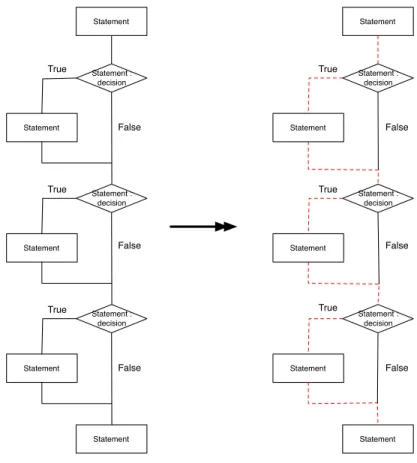
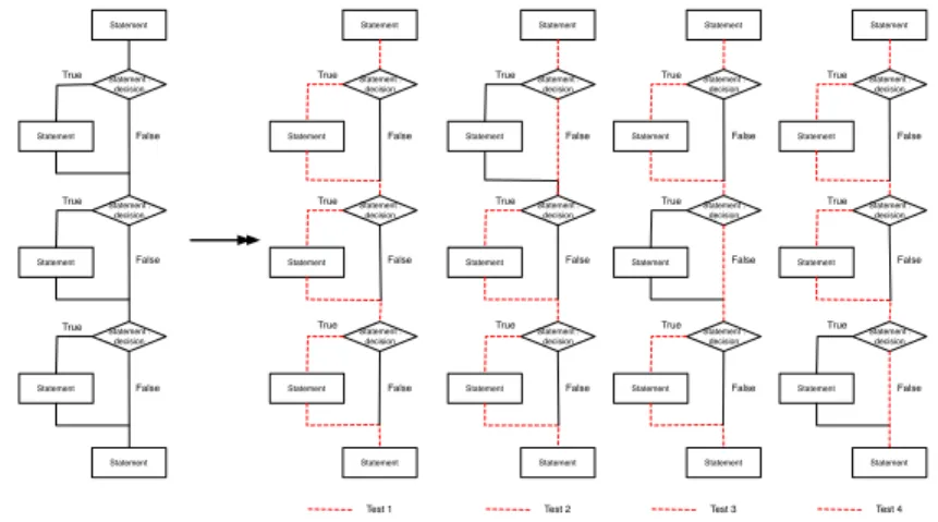
Statement Statement : decision Statement Statement : decision Statement Statement : decision Statement Statement Statement Statement : decision Statement Statement : decision Statement Statement : decision Statement Statement True False True True False False True True True False False False
Figure 3.1: Paths considered by Statement Coverage at 100%.
Definition This suite of metrics assesses how testing covers different parts of the source code, which gives a measure of quality through confidence in code. Unit tests are performed to check code against computable specifications and to determine the reliability of the system. Different metrics evaluate different manners of covering the code.
Scope Project, Method
Analysis There are three principal kinds of coverage:
– Statement Coverage: This metric computes the number of lines of code covered by tests. But there is no guarantee of quality even if the cover-age is 100 %. Covering all lines of code is useful to research broken code or useless code but it does not determine if the returns of the methods are complying with the expectations in all cases. This metric is easy to com-pute but does not take into account execution paths determined by control
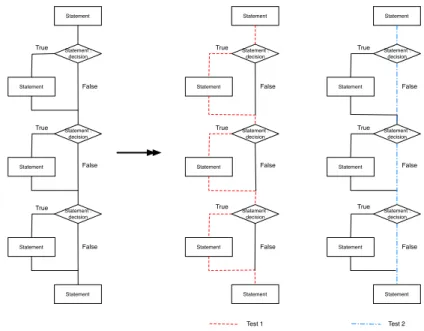
Statement Statement : decision Statement Statement : decision Statement Statement : decision Statement Statement Statement Statement : decision Statement Statement : decision Statement Statement : decision Statement Statement True False True True False False True True True False False False Statement Statement : decision Statement Statement : decision Statement Statement : decision Statement Statement True True True False False False Test 1 Test 2
Figure 3.2: Paths considered by Branch Coverage at 100%.
structures. In Figure 3.1, Statement Coverage is 100 % because all state-ments are covered but there are still three paths which are not covered: the three False paths.
– Branch Coverage or Decision Coverage: This metric determines if tests cover the different branches introduced by the control structures in a sys-tem. For example, an ’if’ introduces two branches and unit tests must in-clude the two cases: True and False. In Figure 3.2, the three control struc-tures introduce six branches and tests must include six cases: True and False for each control structure. So if tests cover the three True branches and then the three False branches, Branch Coverage is 100 % but does not take care of all possible paths in the system: what about the case True, True and False or False, True and True for example?
– Path Coverage: This metric determines if the tests cover all the possible paths in a system. Because of the number of possible paths in a system could be really high (for N conditions there is 2N possible paths) or
un-bounded (if there is an infinite loop), this metric is coupled with the cy-clomatic complexity. The number of paths to cover increases linearly with cyclomatic complexity, not exponentially. Generally, the cyclomatic com-plexity form’s is v(G) = d + 1 where d is the number of binary decision node in G (G could be a method for example). In Figure 3.3 there are three conditions so there are 23= 8 possible paths, but only four paths to cover
Statement Statement : decision Statement Statement : decision Statement Statement : decision Statement Statement Statement Statement : decision Statement Statement : decision Statement Statement : decision Statement Statement True False True True False False True True True False False False Statement Statement : decision Statement Statement : decision Statement Statement : decision Statement Statement True True True False False False Test 1 Test 2 Statement Statement : decision Statement Statement : decision Statement Statement : decision Statement Statement True True True False False False Test 3 Statement Statement : decision Statement Statement : decision Statement Statement : decision Statement Statement True True True False False False Test 4
Figure 3.3: Paths considered by Path Coverage at 100%.
with cyclomatic complexity: 3 + 1. A set of paths could be: True-True-True, False-True-True-True-True, True-False-True-True-True, True-True-False. The other paths are not independent paths so they are ignored.
These metrics indicate the level of tests but not the quality of them. They do not determine if the unit tests are well defined and a number value near 100% does not indicate that there are no more bugs in the source code.
3.2
Design Metrics
Design metrics deal with design principles. They quantify over source code entities to assess whether a source code entity is following a design principle. In particular, such metrics can be used to track down bad design, which correction could lead to an overall improvement.
3.2.1
Class Coupling
High quality software design, among many other principles, should obey the prin-ciple of low coupling. Stevens et al. [SMC74], who first introduced coupling in the context of structured development techniques, define coupling as “the measure of the strength of association established by a connection from one module to another”. There-fore, the stronger the coupling between modules, i.e., the more interrelated they are, the more difficult these modules are to understand, change, and correct and thus the more complex the resulting software system.
Excessive coupling indicates the weakness of class encapsulation and may inhibit reuse. High coupling also indicates that more faults may be introduced due to inter-class activities. A inter-classic example is the coupling between object inter-classes (CBO), which considers the number of other classes “used” by this class. High CBO measure for a class means that it is highly coupled with other classes.
Names Coupling Between Object classes
Acronyms CBO
References [CK94, FP96, Mar05]
Definition Two classes are coupled together if one of them uses the other, i.e., one class calls a method or accesses an attribute of the other class. Coupling involving inheritance and methods polymorphically called are taken into account. CBO for a class is the number of classes to which it is coupled.
Scope Class
Analysis Excessive coupling is detrimental to modular design and prevents reuse. The
more independent a class is, the easier it is to reuse it in another application. Strong coupling complicates a system, since a module is harder to understand, change, and correct by itself if it is interrelated with other modules. CBO evalu-ates efficiency and reusability.
In a previous definition of CBO, coupling related to inheritance was explicitly excluded from the formula.
CBO only measures direct coupling. Let us consider three classes, A, B and C, with A coupled to B and B coupled to C. Depending on the case, it can hap-pen that A dehap-pends on C through B. Yet, CBO does not account for the higher coupling of A in this case.
CBO is different from Efferent Coupling (which only counts outgoing dependen-cies) as well as Afferent Coupling (which only counts incoming dependendependen-cies).
Names Coupling Factor
Acronyms COF
References [BGE95],[BDW99]
Definition Coupling Factor is a metric defined at program scope and not at class scope. Coupling Factor is a normalized ratio between the number of client relationships and the total number of possible client relationships. A client relationship exists whenever a class references a method or attribute of another class, except if the client class is a descendant of the target class. Thus, inheritance coupling is excluded but polymorphically invoked methods are still accounted for.
The formal definition of COF given by Briand et al. [BDW99], for a program composed of a set T C of classes, is:
COF (T C) = P
c∈T C| {d | d ∈ (T C − {c} ∪ Ancestors(c)) ∧ uses(c, d)} |
| T C |2− | T C | −2P
c∈T C| Descendants(c) |
uses(c,d)is a predicate which is true whenever class c references a method or attribute of class d, including polymorphically invoked methods.
Scope Program
Analysis Coupling Factor is a metric which is only defined at program scope and not at class scope. It makes it difficult to compare with metrics defined at class scope, which can only be summarized at program level.
The original metric was unclear whether polymorphic methods should be ac-counted for [BGE95].
Names Message Passing Coupling
Acronyms MPC
References [LH93]
Definition MPC is defined as the “number of send statements defined in a class”. The au-thors further refine the definition by indicating that calls to class own methods are excluded from the count, and that only calls from local methods are considered, excluding calls in inherited methods.
The formal definition of MPC is: M P C(c) = X m∈MI(c) X m0∈SIM (m)−M I(c) N SI(m, m0)
where m belongs to the set of local methods MI and m0 belongs to the set of
methods statically invoked by m (i.e., without taking polymorphism into
ac-count), and excluding local methods (SIM (m) − MI). N SI(m, m0) is the
number of static invocations from m to m0.
Scope Class
Analysis The authors give the following interpretation: “The number of send statements sent out from a class may indicate how dependent the implementation of the local methods is on the methods in other classes.”
MPC does not consider polymorphism as only send statements are accounted for, not method definitions which could be polymorphically invoked.
3.2.2
Class Cohesion
Cohesiveness of methods within a class is desirable since it promotes encapsulation and lack of cohesion implies that classes should probably be split into two or more sub-classes. For example, although we can have more definitions for the lack of cohesion metric, they all show the cohesiveness of the class considering different relationships between the methods of the class. We distinguish class cohesion from package cohe-sion, since late-binding in object-oriented context may lead to good packages that have a low-cohesion as for example in the case of framework extensions.
The Lack of Cohesion in Methods (LCOM) metric was one of the first metric to evaluate cohesion in object-oriented code, based on a similar metric for procedural cohesion. Different versions of LCOM have been released across the years: some have been intended to correct and replace previous faulty versions, while others have taken a different approach to measure cohesion. As a consequence, numbering schemas for LCOM have diverged across references. Typically, LCOM1 was first called LCOM before being replaced by another LCOM, which was later renamed as LCOM2.
Most of the LCOM metrics are somehow naive in the intention that they want to capture: a cohesive class is not a class whose all methods access all the instance variables even indirectly. Most of the time, a class can have state that is central to the the domain it represents, then it may have peripheral state that may be used to share data between computation performed by the methods. This does not mean that the class should be split. Splitting a class is only possible when two groups of attributes and methods are not accessed simultaneously.
All LCOM metrics (LCOM1 to LCOM5) give inverse cohesion measures: a high cohesion is indicated by a low value, and a low cohesion is indicated by a high value. We followed the numbering of LCOM metrics given by [BDW98], which seems the most widely accepted.
Original LCOM definitions only consider methods and attributes defined in the class. Thus inherited methods and attributes are excluded.
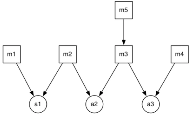
a1 a2 a3
m1 m2 m3 m4
m5
Figure 3.4: Sample graph for LCOM metrics with methods miaccessing attributes aj
Names Lack of Cohesion in Methods
Acronyms LCOM1
References [CK94][BDW98]
Definition LCOM1 is the number of pairs of methods in a class which do not reference a
common attribute.
Scope Class
Analysis In Figure 3.4, LCOM 1 = 7. The pairs without a common attribute are (m1,
m3), (m1, m4), (m2, m4), (m5, m1), (m5, m2), (m5, m3), (m5, m4).
The definition of this metric is naive and led to a lot of debate against it. In general it should be avoided as much as possible. In particular, it does not make sense that all methods of a class directly access all attributes of the class. It can give the same measure for classes with very different designs. This metric gives incorrect results when there are accessor methods.
This metric only considers methods implemented in the class and only refer-ences to attributes implemented in the class. Inherited methods and attributes are excluded.
Names Lack of Cohesion in Methods
Acronyms LCOM2
References [BDW98]
Definition For each pair of methods in the class, if they access disjoint sets of instance variables, then P is increased by one, else Q is increased by one.
– LCOM 2 = P − Q , if P > Q, – LCOM 2 = 0 otherwise,
LCOM 2 = 0 indicates a cohesive class. LCOM 2 > 0 indicates that the class can be split into two or more classes, since its instance variables belong to dis-joint sets.
Scope Class
Analysis In the Figure 3.4, LCOM 2 = 4. P is the sum of all pairs of methods which
reference no common attribute thus P = 7 (pairs (m1, m3), (m1, m4), (m2, m4), (m5, m1), (m5, m2), (m5, m3), (m5, m4)). Q is calculated with other pairs ((m1, m2), (m2, m3), (m3, m4)), thus Q = 3. The result is P − Q = 4.
The definition of LCOM2 only considers methods implemented in the class and references to attributes implemented in the class. Inherited methods and at-tributes are excluded.
It can give the same measure for classes with very different design. LCOM2 may be equals to 0 for many different classes. This metric gives incorrect results when there are accessors methods. Moreover, LCOM2 is not monotonic because of "if Q > P , then LCOM 2 = 0".
Names Lack of Cohesion in Methods
Acronyms LCOM3
References [BDW98]
Definition LCOM3 is the number of connected components in a graph of methods. Methods
are connected in the graph with methods accessing the same attribute.
Scope Class
Analysis In Figure 3.4, LCOM 3 = 2. The first component is (m1, m2, m3, m4)
be-cause these methods are directly or indirectly connected together through some attributes. The second component is (m5) because the method does not access any attribute and thus is not connected.
This metric only considers methods implemented in the class and only refer-ences to attributes implemented in the class. Inherited methods and attributes are excluded.
This metric gives incorrect results when there are accessor methods because only methods directly connected with attributes are considered.
Constructors are a problem, because of indirect connections with attributes. They create indirect connections between methods which use different attributes, and increase cohesion, which is not real.
Names Lack of Cohesion in Methods
Acronyms LCOM4
References [BDW98]
Definition LCOM4 is the number of connected components in a graph of methods. Methods
are connected in the graph with methods accessing the same attribute or calling them. LCOM4 improves upon LCOM3 by taking into account the transitive call graph.
– LCOM 4 = 1 indicates a cohesive class.
– LCOM 4 ≥ 2 indicates a problem. The class should be split into smaller classes.
– LCOM 4 = 0 happens when there are no methods in a class.
Scope Class
Analysis In the Figure 3.4, LCOM4 = 1. The only component is (m1, m2, m3, m4, m5)
because these methods are directly or indirectly connected to the same collection of attributes.
If there are 2 or more components, the class could be split into smaller classes, each one encapsulating a connected component.
Names Lack of Cohesion in Methods
Acronyms LCOM5, LCOM*
References [BDW98] Definition LCOM 5 = N OM − P m∈MN OAcc(m) N OA N OM − 1
where M is the set of methods of the class, N OM the number of methods, N OA the number of attributes, and N OAcc(m) is the number of attributes of the class accessed by method m.
Scope Class
Analysis In Figure 3.4, LCOM5 =34, because N OM = 5, N OA = 3,P N OAcc = 6.
A common acronym for LCOM5 is LCOM*.
LCOM5 varies in the range [0,1]. It is normalized compared to others LCOM or TCC and LCC which have no upper limit of the values measured. But LCOM5 can return a measure up to two when there is for example only two methods and no attribute accesses.
This metric considers that each method should access all attributes in a com-pletely cohesive class, which is not a good design.
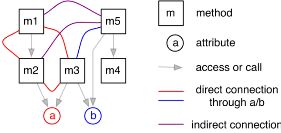
Names Tight Class Cohesion
Acronyms TCC
Definition TCC is the normalized ratio between the number of methods directly connected with other methods through an instance variable and the total number of possible connections between methods.
A direct connection between two methods exists if both access the same instance variable directly or indirectly through a method call (see Figure 3.5).
– N P = N ×(N −1)2 : maximum number of possible connections where N is
the number of visible methods – N DC: number of direct connections – T CC = N DCN P
TCC takes its value in the range [0, 1].
For TCC only visible methods are considered, i.e., they are not private or imple-ment an interface or handle an event. Constructors and destructors are ignored.
Scope Class
Analysis TCC measures a strict degree of connectivity between visible methods of a class. TCC satisfies all cohesion properties defined in [BDW98].
The higher TCC is, the more cohesive the class is. According to the authors, T CC < 0.5 points to a non-cohesive class. T CC = LCC = 1 is a maximally cohesive class: all methods are connected.
Constructors are a problem, because of indirect connections with attributes. They create indirect connections between methods which use different attributes, and increase cohesion, which is not real.
Names Loose Class Cohesion
Acronyms LCC
References [BK95, BDW98]
Definition LCC is the normalized ratio between the number of methods directly or indirectly connected with other methods through an instance variable and the total number of possible connections between methods.
There is an indirect connection between two methods if there is a path of direct connections between them. It is defined using the transitive closure of the direct connection graph used for TCC (see Figure 3.5).
– N P = N ×(N −1)2 : maximum number of possible connections where N is
the number of visible methods – N IC: number of indirect connections
m2
m3
m4
m1
a
b
m5
m
method
a
attribute
access or call
direct connection
through a/b
indirect connection
Figure 3.5: In this example depicting five methods and two attributes of a class, we have T CC = 104 (counting red and blue lines) and LCC = 106 (adding purple lines to the count).
– LCC = N DC+N ICN P
– By definition, LCC ≥ T CC LCC takes its value in the range [0, 1].
For LCC only visible methods are considered, i.e., they are not private or imple-ment an interface or handle an event. Constructors and destructors are ignored.
Scope Class
Analysis LCC measures an overall degree of connectivity between visible methods of a
class. LCC satisfies all cohesion properties defined in [BDW98].
The higher LCC is, the more cohesive the class is. According to the authors, LCC < 0.5 points to a non-cohesive class. LCC = 0.8 is considered “quite co-hesive”. T CC = LCC indicates a class with only direct connections. T CC = LCC = 1 is a maximally cohesive class: all methods are connected.
Constructors are a problem, because of indirect connections with attributes. They create indirect connections between methods which use different attributes, and increase cohesion, which is not real.
3.2.3
Package Architecture
Package Design Principles. R.C. Martin discussed principles of architecture and package design in [Mar97, Mar05, Mar00]. He proposes several principles:
• Release / Reuse Equivalence principle (REP): The granule of reuse is the granule of release. A good package should contain classes that are reusable together. • Common Reuse Principle (CRP): Classes that are not reused together should not
be grouped together.
• Common Closure Principle (CCP): Classes that change together, belong together. To minimize the number of packages that are changed in a release cycle, a pack-age should contain classes that change together.
• Acyclic Dependencies Principle (ADP): The dependencies between packages must not form cycles.
• Stable Dependencies Principle (SDP): Depend in the direction of stability. The stability is related to the amount of work required to make a change on it. Con-sequently, it is related to the package size and its complexity, but also to the number of packages which depend on it. So, a package with lots of incoming dependencies from others packages is stable (it is responsible to those packages); and a packages with not any incoming dependency is considered as independent and unstable.
• Stable Abstractions Principle (SAP): Stable packages should be abstract pack-ages. To improve the flexibility of applications, unstable packages should be easy to change, and stable packages should be easy to extend, consequently they should be highly abstract.
Some metrics have been built to assess such principles: For example, the Abstract-ness and Instability metrics are used to check SAP.
Martin Package Metrics. The following metrics defined by Martin [Mar97] aim at characterizing good design in packages along the SDP and SAP principles. However, the measurements provided by the metrics are difficult to interpret.
Names Efferent Coupling (module)
Acronyms Ce
References [?]
Definition Efferent coupling for a module is the number of modules it depends upon (out-going dependencies, fan-out, Figure 3.6).
Analysis In [Mar00], efferent coupling for a package was defined as the number of classes outside the package that classes inside depend upon. In [Mar97], efferent cou-pling for a package was defined as the number of classes in the package which depend upon classes external to the package.
The current definition is generalized with respect to the concept of module, where a module is always a class or always a package.
Names Afferent Coupling (module)
Acronyms Ca
References [?]
Definition Afferent coupling for a module is the number of modules that depend upon this module (incoming dependencies, fan-in, Figure 3.6).
Scope Class, Package
Analysis In [Mar97], afferent coupling for a package was defined as the number of classes external to the package which depend upon classes in the package.
Names Abstractness
Acronyms A
References [Mar97]
Definition Abstractness is the ratio between the number of abstract classes and the total number of classes in a package, in the range [0, 1]. 0 means the package is fully concrete, 1 it is fully abstract.
Scope Package
Analysis This metric can not be analyzed in isolation. In any system, some packages
should be abstract while other should be concrete.
Names Instability
Acronyms I
Figure 3.6: Each module is represented by a box with enclosed squares. It is either a class enclosing methods and attributes, or a package enclosing classes. Efferent cou-pling is the number of red modules (Ca = 2); afferent coucou-pling is the number of blue modules (Ce = 2).
Definition I = Ce(P )+Ca(P )Ce(P ) , in the range [0, 1]. 0 means package is maximally stable (i.e., no dependency to other packages and can not change without big consequences), 1 means it is unstable.
This metric is used to assess the Stable Dependencies Principle (SDP): according to Martin [Mar97], a package should only depends on packages which are more stable than itself, i.e. it should have a higher I value than any of its dependency. The metric only gives a raw value to be used while checking this rule.
Scope Package
Analysis Instability is not a measure of the possibility of internal changes in the package, but of the potential impact of a change related to the package. A maximally sta-ble package can still change internally but should not as it will have an impact on dependent packages. An unstable package can change internally without conse-quences on other packages. Intermediate values, in the range ]0, 1[], are difficult to interpret.
A better way to understand Instability is as a Responsible/Independent couple. A stable package (I = 0) is independent and should be responsible because of possible incoming dependencies. An unstable package is dependent of other packages and not responsible for other packages.
The stability concept, understood as sensitivity to change, should be transitively defined: a package can only be stable if its dependencies are themselves stable.
Names Distance
Acronyms D
References [Mar97]
Definition D = A+I−1√
2 or (normalized) D
0 = A + I − 1. A package should be balanced
between abstractness and instability, i.e., somewhere between abstract and stable or concrete and unstable. This rule defines the main sequence by the equation A + I − 1 = 0. D is the distance to the main sequence.
This metric is used to assess the Stable Abstractions Principle (SAP): stable packages should also be abstract packages (A = 1 and I = 0) while unstable packages should be concrete (A = 0 and I = 1).
Scope Package
Analysis This metric assumes a one-to-one inverse correlation between Abstractness and Instability to assert the good design of a package. However, such a correlation seems uneasy given the difference in data nature on which each metric is com-puted. To our knowledge, no large scale empirical study has been performed to confirm this assumption.
This metric is sensitive to extreme cases. For example, a package with only concrete classes (A = 0) but without outgoing dependencies (I = 0) would have a distance D0 = −1. Yet this package does not necessarily exhibit a bad design.
3.3
New Metrics and Missing Aspects
A Few Thoughts about Package Characterization.
Package characterization by metrics is still a new topic in the context of software engineering. The following items sum up some of the challenges that package metrics will be confronted to.
• Class cohesion does not translate to package level: sets of cohesive classes do not make necessarily a cohesive package;
• Package cohesion and coupling can be improved by moving classes around, or possibly refactoring some classes to improve their own cohesion or coupling — worst case, a class needs to be split so as to remove a dependency into another class;
• Late-binding allows subclasses to extend or refine superclasses. This is not clear that packages extending classes have to be cohesive.
• Given that the cost of maintenance of a package can vary greatly depending on its contents and relationships, it is necessary to have some metrics to assess the complexity of a package.
The second item asks for special attention: there is a transition between the package level and the class level. When targeting a package, we need to assess whether the source of bad cohesion/coupling arises from bad class placement, each class being in itself cohesive, or from bad design in a class which shows signs of low cohesion and high coupling with another package. Package can be improved in the first case by moving classes around, or in the second case such classes must be refactored first. It is not clear how package-level metrics could discriminate between such cases.
The following define a set of primitive metrics that capture some package charac-teristics.
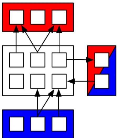
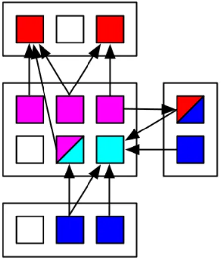
Figure 3.7: This figure illustrates some primitive metrics for packages. With
re-spect to the central package: N CP (N umber of classes in package) = 6;
HC(Hidden classes) = 1; OutC(package provider classes) = 4 (magenta); InC(P ackage used classes) = 2 (cyan); SP C(System provider classes) = 3 (red); SCC(System client classes) = 4 (blue).
3.3.1
Package Primitive Metrics.
Currently, primitive metrics for package characterisation are not standardized or simply missing.
Package building is less driven by the principles of data abstraction and encapsu-lation, as for classes, than by the idea of grouping a set of classes as a subsystem with common purpose. Thus, a package can not be characterized as the sum of of its classes. Therefore, the use of statistical formula (mean, max, sum) to compute package level measures can hide important facts about the package itself. However, statistical for-mula are still useful to select classes when inspecting the internals of a package, which can be helpful to improve the overall package in some cases.
Names Number of Classes in Package (Package size)
Acronyms NCP
References [Abd09]
Definition N CP is the number of classes packaged inside the package. It is a primitive metric.
Analysis
Names Out-port Classes
Acronyms OutC
References [Abd09]
Definition OutC is the number of classes in the package that have outgoing edges to pack-age external classes i.e., packpack-age provider classes.
Scope Package
Analysis This is not the same as efferent coupling.
Names In-port Classes (Package used classes)
Acronyms InC
References [Abd09]
Definition InC is the number of classes in the package that have incoming edges from
classes out of the package i.e., client classes.
Scope Package
Analysis This is not the same as afferent coupling.
Names Hidden Classes
Acronyms HC
References [Abd09]
Definition HC is the number of classes in the package that have no edge related to classes out of the package.
Scope Package
Analysis
Acronyms SPC
References [Abd09]
Definition SP C is the number of classes out of the package which package classes depend upon.
Scope Package
Analysis This is not the same as efferent coupling.
Names System Client Classes
Acronyms SCC
References [Abd09]
Definition SCC is the number of classes out of the package which depend upon package
classes.
Scope Package
Analysis This is not the same as afferent coupling.
3.3.2
System Package Primitive Metrics.
Now the class metrics are lifted at the package level.
Names Provider Packages
Acronyms PP
References [Abd09]
Definition P P is the number of packages which the package depends upon.
Scope Package
Analysis This is efferent coupling (Ce) at the package level.
Names Client Packages
Acronyms CP
Definition CP is the number of packages which depend upon the package.
Scope Package
Analysis This is afferent coupling (Ca) at the package level.
Names Package Relative Importance for System
Acronyms PRIS
References [Abd09]
Definition P RIS = N umberOf P ackagesInT heSystem−1CP . This metric takes its values be-tween 0 and 1.
Scope Package
Analysis It helps to rank a package by its importance in the system according to its afferent coupling, i.e., the number of its clients.
Names System Relative Importance for Package
Acronyms SRIP
References [Abd09]
Definition SRIP = N umberOf P ackagesInT heSystem−1P P . This metric takes its values be-tween 0 and 1.
Scope Package
Analysis It helps to rank a package by its dependence on the system according to its effer-ent coupling, i.e., the number of its providers.
Names Number of Package in Cyclic Dependency
Acronyms NPCD
References [Abd09]
Definition N P CD is the number of packages which play, at the same time, a role of client and provider to the considered package.
Analysis They are all the packages which have cyclic dependencies with the considered package.
Names Number of Packages in Dependencies
Acronyms NPD
References [Abd09]
Definition N P D = CP +P P −P RI is the number of all packages related to the concerned package (client and provider packages). We subtract P RI from the sum because packages in cyclic dependencies are counted two times in CP + P P .
Scope Package
Analysis If we consider that each client/provider package presents some services of the concerned package thus this metric gives an idea about the package aspects and their distribution in the system. In consequence, it gives an idea about the com-plexity of the package services and responsibilities.
3.3.3
Package Cohesion
There is no agreement on what makes a package cohesive. Actually, some au-thors [Mis01, Pon06]) think that cohesion for a package cannot be determined from the internal structure of the package alone: one must consider the context, i.e., what the package uses and how it is used. A set of cohesive classes does not necessarily make a package cohesive. For example, the package can have different clients using specifically different set of the package.
In addition, class-level cohesion metrics do not necessarily translate at the package level. For example, a package where classes would not share any relationships between them, but would inherit from a common external superclass, can be a proper package.
Ponisio [Pon06] et al. introduce the idea of using the context of a package, i.e., its dependencies, rather than simply its internal structure, to characterize a package cohe-sion. Classes can belong together in a cohesive package even without a dependency between them, because they are accessed by the same external classes. They propose the Contextual Package Cohesion metric to characterize such a cohesion. In particu-lar, the Contextual Package Cohesion metric can be used to assess the Common Reuse Principle.
Names Contextual Package Cohesion. Locality
Acronyms CPC
Definition The CPC metric is based on the concept of similarity between pairs of objects. The more client packages use the same classes in the package, the more cohesive the package is (see Figure 3.8).
Contextual Package Cohesion is the ratio between the number of pairs of classes which are referenced by a common client package, and the total number of pos-sible pairs of classes in a package interface. The package interface includes all classes which external classes depend upon. With CPC, a cohesive package is one where classes in the package interface are depended upon by a common set of packages.
– classes(P ) retrieve the set of classes defined in package P .
– I = {c|c ∈ P ∧clientClasses(c)−classes(P ) 6= ∅}: interface of package P , i.e., classes which external classes depend upon.
– N P = |I|×(|I|−1)2 : maximum number of possible pairs formed by classes of the package interface.
– f (a, b) = 1
if (clientP ackages(a) − P ) ∩ (clientP ackages(b) − P ) 6= ∅,
f (a, b) = 0 otherwise – CP C = P a,b∈If (a,b) N P Scope Package
Analysis CPC focuses on classes at the interface of the package and external clients and normalizes its measure in the range [0, 1].
The original definition of the client relationship by [Pon06] was unsound be-cause it mixes classes and packages. We refine those definition with two dis-tinct functions, clientClasses(c) which retrieve classes referencing class c, and clientP ackages(c) which retrieve packages referencing class c. clientClasses can include other classes of P as well as clientP ackages can include P itself so those internal references must be excluded from the relationships.
Names Locality
Acronyms
References [Pon06]
Definition Locality for a class is described as Contextual Package Cohesion evaluated us-ing reference dependencies. However, the current formula for CP C cannot be applied at class level. Locality for a class can be roughly described as how well a class matches with other classes of its package in terms of client usage.
D
A
B
C
P
R
S
Q
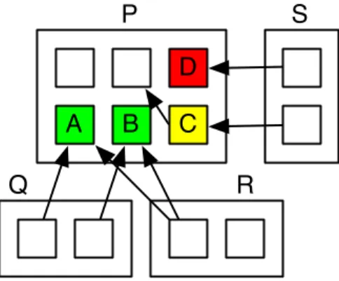
Figure 3.8: Classes A, B, C, D constitute the interface of package P. Classes A and B are both referenced together by packages Q and R, making this part of P cohesive. On the contrary, classes C and D are only used by package S and thus are misplaced (Locality). However, only D can be moved freely, as C also references an internal class of package P (Happiness). In this example CP C = 16. Moving class D would increase cohesion up to 13.
Analysis Locality could be used to refine CPC interpretation by pointing to classes which are misplaced in the package because they have different external clients than other package classes. Yet no known definition exists for this metric.
Names Happiness
Acronyms
References [Pon06]
Definition Happiness for a class measures how well a class fits in a package. It is based on the class coupling with other classes in the package. Although no formal definition is given, a tentative definition would be afferent coupling of a class within its package, i.e., the number of client classes inside its package.
Scope Class
Analysis Happiness is a metric used to counterbalance Locality in package refactoring. Locality points to classes which are misplaced in the package because they have different external clients. However a misplaced class which also have internal dependencies (hence high Happiness measure) should not necessarily be moved.
Chapter4. Conclusion
This document presents a selection of metrics that can be useful to characterize object-oriented systems. They range from simple mere measurements to more sophisticated metrics. The goal of this document is not to have a long catalog but to select some metrics, either because they were commonly used, debated (LCOM), or because they represent important aspects of an OO system in terms of its quality (package cohesion). The current catalog of metrics is intended to be used to define practices in the Squale four level quality model. The second level called practices are smart aggregation of metrics and will be the focus of deliverable 1.3.
Bibliography
[Abd09] Hani Abdeen. Visualizing, Assessing and Re-Modularizing
Object-Oriented Architectural Elements. PhD thesis, Université of Lille, 2009. [BDPW98] L.C. Briand, J. Daly, V. Porter, and J. Wust. A comprehensive
empir-ical validation of design measures for object-oriented systems. Software Metrics Symposium, 1998. Metrics 1998. Proceedings. Fifth International, pages 246–257, Nov 1998.
[BDW98] Lionel C. Briand, John W. Daly, and Jürgen Wüst. A Unified Framework
for Cohesion Measurement in Object-Oriented Systems. Empirical Soft-ware Engineering: An International Journal, 3(1):65–117, 1998.
[BDW99] Lionel C. Briand, John W. Daly, and Jürgen K. Wüst. A Unified
Frame-work for Coupling Measurement in Object-Oriented Systems. IEEE
Transactions on Software Engineering, 25(1):91–121, 1999.
[BGE95] F. Brito e Abreu, M. Goulao, and R. Esteves. Toward the design quality
evaluation of object-oriented software systems. In Proc. 5th Int’l Conf. Software Quality, pages 44–57, October 1995.
[BK95] J.M. Bieman and B.K. Kang. Cohesion and reuse in an object-oriented
system. In Proceedings ACM Symposium on Software Reusability, April 1995.
[BMB96] Lionel C. Briand, Sandro Morasca, and Victor Basili. Property-based
soft-ware engineering measurement. Transactions on Softsoft-ware Engineering, 22(1):68–86, 1996.
[CK94] Shyam R. Chidamber and Chris F. Kemerer. A metrics suite for object
oriented design. IEEE Transactions on Software Engineering, 20(6):476– 493, June 1994.
[FP96] Norman Fenton and Shari Lawrence Pfleeger. Software Metrics: A
Rig-orous and Practical Approach. International Thomson Computer Press, London, UK, second edition, 1996.
[GFS05] Tibor Gyimóthy, Rudolf Ferenc, and Istvá Siket. Empirical validation of
object-oriented metrics on open source software for fault prediction. IEEE Transactions on Software Engineering, 31(10):897–910, 2005.
[HK00] Jiawei Han and Micheline Kamber. Data Mining: Concept and
Tech-niques. Morgan Kaufmann, 2000.
[HM95] Martin Hitz and Behzad Montazeri. Measuring product attributes of
object-oriented systems. In Proc. ESEC ‘95 (5th European Software En-gineering Conference, pages 124–136. Springer Verlag, 1995.
[HS96] Brian Henderson-Sellers. Object-Oriented Metrics: Measures of Com-plexity. Prentice-Hall, 1996.
[Kan02] Stephen H. Kan. Metrics and Models in Software Quality Engineering.
Addison Wesley, 2002.
[LH93] W. Li and S. Henry. Object oriented metrics that predict maintainability.
Journal of System Software, 23(2):111–122, 1993.
[LK94] Mark Lorenz and Jeff Kidd. Object-Oriented Software Metrics: A
Practi-cal Guide. Prentice-Hall, 1994.
[LM06] Michele Lanza and Radu Marinescu. Object-Oriented Metrics in Practice.
Springer-Verlag, 2006.
[Mar97] Robert C. Martin. Stability, 1997. www.objectmentor.com.
[Mar00] Robert C. Martin. Design principles and design patterns, 2000.
www.objectmentor.com.
[Mar05] Robert C. Martin. The tipping point: Stability and instability in oo design, 2005. http://www.ddj.com/architect/184415285.
[May99] Tobias Mayer. Only connect. an investigation into the relationship between object-oriented design metrics and the hacking culture, 1999.
[McC76] T.J. McCabe. A measure of complexity. IEEE Transactions on Software
Engineering, 2(4):308–320, December 1976.
[Mis01] Vojislav B. Misi´c. Cohesion is structural, coherence is functional: Differ-ent views, differDiffer-ent measures. In Proceedings of the SevDiffer-enth International Software Metrics Symposium (METRICS-01). IEEE, 2001.
[MR04] Radu Marinescu and Daniel Ra¸tiu. Quantifying the quality of
object-oriented design: the factor-strategy model. In Proceedings 11th Work-ing Conference on Reverse EngineerWork-ing (WCRE’04), pages 192–201, Los Alamitos CA, 2004. IEEE Computer Society Press.
[Pon06] María Laura Ponisio. Exploiting Client Usage to Manage Program
Mod-ularity. PhD thesis, University of Bern, Bern, June 2006.
[SMC74] W. P. Stevens, G. J. Myers, and L. L. Constantine. Structured design. IBM
Systems Journal, 13(2):115–139, 1974.
[TNM08] Ewan Tempero, James Noble, and Hayden Melton. How do java
pro-grams use inheritance? an empirical study of inheritance in java soft-ware. In ECOOP ’08: Proceedings of the 22nd European conference on Object-Oriented Programming, pages 667–691, Berlin, Heidelberg, 2008. Springer-Verlag.