HAL Id: hal-00697218
https://hal.archives-ouvertes.fr/hal-00697218v2
Preprint submitted on 3 Jul 2012
HAL is a multi-disciplinary open access
archive for the deposit and dissemination of sci-entific research documents, whether they are pub-lished or not. The documents may come from teaching and research institutions in France or abroad, or from public or private research centers.
L’archive ouverte pluridisciplinaire HAL, est destinée au dépôt et à la diffusion de documents scientifiques de niveau recherche, publiés ou non, émanant des établissements d’enseignement et de recherche français ou étrangers, des laboratoires publics ou privés.
Isabelle Abraham, Romain Abraham, Maïtine Bergounioux
To cite this version:
Isabelle Abraham, Romain Abraham, Maïtine Bergounioux. A variational method for tomographic reconstruction with few views. 2012. �hal-00697218v2�
Inverse Problems in Science and Engineering Vol. 00, No. 00, July 2012, 1–25
RESEARCH ARTICLE
A variational method for tomographic reconstruction with few views
I. AbrahamaR. Abrahamband M. Bergouniouxb∗
aCEA Ile de France- BP 12, 91680 Bruy`eres le Chˆatel, France ;bUniversit´e d’Orl´eans,
UFR Sciences, MAPMO, UMR 7349, Route de Chartres, BP 6759, 45067 Orl´eans cedex 2, France
(v1.2 released July 3, 2012)
In this article, we focus on tomographic reconstruction. The problem is to determine the shape of the interior interface using a tomographic approach while very few X-ray radiographs are performed. We present a variational model and numerical analysis. We use a modified Nesterov algorithm to compute the solution. Numerical results are presented.
Keywords: Inverse problem, Tomography, Variational model AMS Subject Classification: 49N45, 35A15,65J22,94A08
1. Introduction
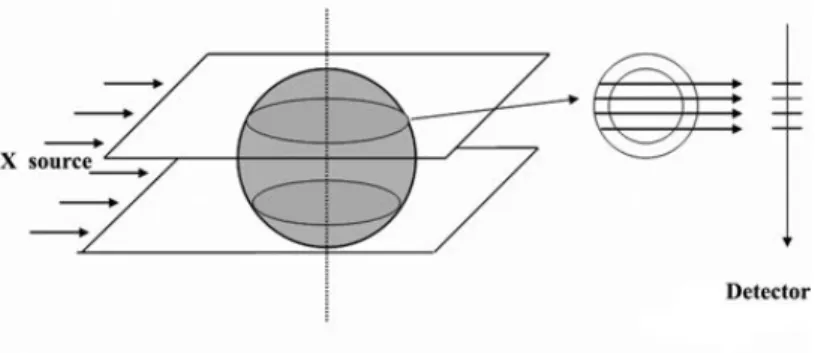
In this article, we focus on a specific application of tomographic reconstruction for a physical experiment whose goal is to study the behavior of a material under a shock. The experiment consists in causing the implosion of the hull of some material (usually, a metal) using surrounding explosives. The problem is to determine the density and the interior interface at a specific moment of the implosion. For this purpose, very few X-ray radiographs are performed, and the density of the object must then be reconstructed using a tomographic approach (see Figure 1.1).
In [1] we mentioned that several techniques exist for tomographic reconstruction, providing an analytic formula for the solution (see for instance [15] or [13]) as soon as a large number of projections of the object, taken from different angles, are available. There is a huge literature about theoretical and practical aspects of the problem of reconstruction from projections, the applications of which concern medicine, optics, material science, astronomy, geophysics, and magnetic resonance imaging (see [7]). When only few projections are known, these methods cannot be used directly, and some alternative methods have been proposed to reconstruct the densities (see for instance [19]).
As in any tomographic reconstruction process, this problem leads to an ill-posed inverse problem. As X-rays must cross a very dense object and only a few number of them arrive at the detector, it is therefore necessary to add some amplification devices and very sensitive detectors, which cause a high noise level [25, 26] .
∗Corresponding author. Email: [email protected]
ISSN: 1741-5977 print/ISSN 1741-5985 online c
� 2012 Taylor & Francis
DOI: 10.1080/1741597YYxxxxxxxx http://www.informaworld.com
Figure 1.1. Tomography experiment
Figure 1.2. Different projections around the tomography axis
The tomographic reconstruction with few views problem has been widely studied. If a large number of radiographs is available, we can use several efficient methods that lead to exact formulas to compute the solution (see [22] or [15]).
Missing data problems can been studied with such methods as well ( [22], chapter 6 or [27]). It is the case, for example, when the object is measured on a subset of its support (so-called inner problem, see for example [12]). These techniques, as, for instance, the back-filtered projection (in the full case) or the back-projection for the projection derivatives (in the missing data case [24]) require a fine sampling of measures (here radiographs) to be performing ([22], chapter 4). Therefore, they are not useful in the case where few projection data are available.
The number of available projections (views) is closely related to the ill-posedness of the reconstruction problem. Indeed, the smaller the number of data is, the larger is the kernel of the related operator. Roughly speaking, there are an infinity of solutions and this infinity is linked to the kernel dimension. Some methods have been proposed that allow a partial reconstruction of the object [19]. In the case where we deal with specific objects there exists methods selecting a solution with respect to some prior : in [18], [17] the authors use a bayesian model while an optimization approach is used in [6],[5] where the problem is modelled as a minimal cost flow problem.
In [1] we have assumed that the components of the initial physical setup (object, hull, explosives, etc) are axially symmetric and remain as such during the implosion process. High speed image capture provides a snapshot of the deformation of an object by X-ray radiography. Since this object is assumed to be axially symmetric, a single radiograph suffices in theory to reconstruct the 3D object. The inverse
problem remains ill-posed : existence and uniqueness of a solution are ensured but there is a lack of stability. However, interesting results have been obtained with a variational method ([1, 8]).
In the present paper, we do not assume that the object is axially symmetric any longer but we have more than one radiograph. However, due to the experimental setup, we only deal with very few radiographs, taken from three angles that we suppose to be 0,π4 and π2 for sake of simplicity. So the prior to choose is not straightforward. The previously quoted methods are efficient as soon as we have much more data sets (projections) than we have. In this paper we propose to use a variational method involving priors that are not necessarily consistent with the physical point of view. Looking for more appropriate models will be done in forthcoming works.
The paper is organized as follows. We first present the direct and inverse problems with some classical methods that are not fruitful in this context. Next section is devoted to the study of a variational model both from the theoretical and numerical points of view. We present a generic algorithm. The last section is devoted to the numerical experiments: discretization process, algorithmic tricks and results.
2. Mathematical modelling of the direct problem
In what follows, we assume that the X-sources are far enough from the object so that we may assume that the X-rays are parallel. Therefore we can separate the horizontal planes and reconstruct them independently (see Figure 2.1).
Figure 2.1. Parallel X-rays : the information along a detector segment depends on a planar slice of the object.
We recall [1] that radiography measures the attenuation of X-rays through the object. Let I0 denote the intensity of the incident X-rays flux. Then, the measured
flux I at a point M of the detector is given by I = I0e−
�
∆µ(�)d�,
where the integral operates along the ray ∆ that reaches the point M of the de-tector, d� is the infinitesimal element of length along the ray, and µ is the linear attenuation coefficient. Considering the Neperian logarithm of this attenuation permits to deal rather with linear operators, and the linear mapping
H : (∆, µ)�−→ H(∆, µ) := �
∆
µ(�) d�
µ(x, y, z). The operator H restricted to any horizontal plane (z constant) coincides with the bidimensional Radon transform of µz. Let us recall its definition [21] :
Definition 2.1: Assume n≥ 2 and define Sn−1 as the unit sphere of n. For any function f ∈ S( n) the Radon transform R is defined as
Rf : Sn−1× →
(ζ, s)�→�x.ζ=sf (x)dx =�ζ⊥f (sζ + y)dy .
where x.ζ stands for nusual inner product and ζ⊥ is the orthogonal subspace to ζ.
Here S( n) is the Schwartz space of C∞, rapidly decreasing functions. For any
f ∈ S( n), Rf belongs to S(Sn−1 × ). If n = 2, the Radon transform of a
function f ∈ S( 2) reads
∀θ ∈ [0, π[, ∀s ∈ Hf (θ, s) = � +∞
−∞
f (t sin(θ)+s cos(θ),−t cos(θ)+s sin(θ)) dt and the relation between R and H is : Hf (θ, s) = Rf (ζ, s) , where ζ = (cos θ, sin θ). So, the reconstruction of the object requires the inversion of the Radon transform restricted to any horizontal slice. Therefore, we focus now on the inversion in the 2D framework. We assume that the object is completely represented by its attenuation coefficient µ proportional to its density ρ : 2 → . We assume in addition that ρ vanishes outside an (2D) open disk Ω = B�.�2(0, a) of center 0 and radius a. Therefore, the support of ρ is included in Ω. Here�.�2 denotes the euclidean norm.
In what follows, we call C0
c(Ω), the space of continuous functions with compact
support in Ω.
Remark 1 : As ρ = 0 outside Ω⊂] − a, a[×] − a, a[, then � Ω ρ(x, y) dx dy = � a −a � a −a ρ(x, y) dx dy as soon as the integrals are defined.
For any θ∈ [0, π[ the Radon transform of ρ ∈ C0
c(Ω), is defined as :
Hρ(θ, s) = � +∞
−∞
ρ(t sin(θ) + s cos(θ),−t cos(θ) + s sin(θ)) dt =
� +a
−a
ρ(t sin(θ) + s cos(θ),−t cos(θ) + s sin(θ)) dt.
It has a compact support included in ]−a, a[. For every θ ∈ [0, π[ let us note Hθ
the operator defined as
Hθρ : → s�→ Hρ(θ, s) . Therefore H0ρ(s) = � +∞ −∞ ρ(t, s) dt = � +a −a ρ(t, s) dt . (2.1)
Let Γθ be the rotation of center (0, 0) and angle θ:
∀ρ ∈ Cc0(Ω), Γθρ(x, y) = ρ(x cos(θ) + y sin(θ),−x sin(θ) + y cos(θ)),
so that the projection operator with angle θ∈ [0, π] is Hθ= H0◦ Γθ:Cc0(Ω)→ Cc0(]−a, a[).
We may extend the operator H0 to L2(Ω) by density with next proposition. In
what follows, for any subset E of s, (·, ·)
L2(E) denotes the L2(E) inner product
and � · �L2(E) the L2(E) hilbertian norm. We note (·, ·)2 and � · �2 when there is
no ambiguity.
Proposition 2.2: The operator Hθ is a bounded linear operator from
� C0 c(Ω),�.�L2(Ω) � to �C0 c(]− a, a[), �.�L2(]−a,a[) � . Proof : Let be ρ∈ C0 c(Ω). Then �H0ρ�2L2 = � a −a � � � � � a −a ρ(x, y)dx � � � � 2 dy = � a −a �
ρ(., y) , 1]−a,a[�2L2(]−a,a[)dy≤ 2a�ρ�
2 L2
by Cauchy-Schwarz inequality. As Γθ is an isometry we have the same result for
Hθ. �
We extend Hθon L2(Ω) by density arguments and we denote similarly the extended
operator. We can define the adjoint operator of H0: H0∗ : L2(]−a, a[) −→ L2(Ω)
such that
∀(v, ρ) ∈ L2(]−a, a[) × L2(Ω) (v , H0ρ)L2(]−a,a[) = (H0∗v , ρ)L2(Ω).
Proposition 2.3: The adjoint operator of H0 is given by
H0∗ : L2(]−a, a[) −→ L2(Ω)
H0∗v(x, y) := 1Ω(x, y)v(y), for a.e. y
where 1Ω is the indicator function of Ω : 1Ω(x, y) =
�
1 if (x, y)∈ Ω 0 else
Proof : Let v∈ L2(]−a, a[), ρ ∈ L2(Ω) and (ρ
n) be a sequence of Cc0(Ω) functions
that converges to ρ in L2(Ω). We get for every n > 0
(H0∗v , ρn)L2(Ω)= (v , H0ρn)L2(]−a,a[) = � a −a v(y)H0ρn(y) dy = � Ω v(y)ρn(x, y) dx dy .
Passing to the limit as n→ +∞ gives the result. �
We deduce Hθ∗ easily : Hθ∗= (H0◦ Γθ)∗= Γ∗θ◦ H0∗ = Γ−θ◦ H0∗ .
3. A variational model
In what follows,{θ0, θ1, . . . , θp−1} denotes the p acquisition angles (in [0, π[). The
measured data are πi(:= Hiρ)∈ L2(]−a, a[) where Hi := Hθi, i = 0,· · · , p − 1. It
Figure 3.1. Example of three different solutions for the same 2-views data set .
As already mentioned, it is hopeless to get exact inversion formulas to solve Hiρ = πi, i = 0,· · · , p − 1.
So we rather use a least square approach to minimize
p−1
�
i=0
�Hiρ− πi�2L2(]−a,a[). As
the kernel of Hi may be quite large , the spaceN = p−1�
i=0
ker Himay be not reduced
to {0} and the functional is not coercive, not strictly convex. More precisely, if any minimizing sequence lies in N it is not possible to prove its convergence. Moreover, even if we get a solution, we dot not have uniqueness. Therefore, we have to add some prior information on ρ . It is classical to consider the total variation of functions, which is an efficient tool to reduce noise, as a penalization term.
3.1. Functional framework
In what follows, E is an open bounded subset of n. We recall here the definition of the the space of bounded variation functions (see [3]):
BV (E) ={u ∈ L1(E)| Φ(u) < +∞}, where
Φ(u) = sup ��
E
u(x) div ξ(x) dx | ξ ∈ Cc1(E), �ξ�∞≤ 1 �
. (3.2)
The application Φ is a semi-norm and the space BV (E), endowed with the norm �u�BV = �u�L1 + Φ(u), is a Banach space. The derivative in the sense of the
distributions of every u∈ BV (E) is a bounded Radon measure, denoted Du, and Φ(u) =�E|Du| is the total variation of Du. We next recall standard properties of bounded variation functions (see [2, 3]).
Proposition 3.1: Let E be an open subset of n with Lipschitz compact
bound-ary.
(1) For every u ∈ BV (E), the Radon measure Du can be decomposed into Du = Du dx + Dsu, where Du dx is the absolutely continuous part of Du
(2) The mapping u �→ Φ(u) is lower semi-continuous (denoted in short lsc) from BV (E) to + for the L1(E) topology.
(3) BV (E)⊂ L1∗
(E) with continuous embedding, where 1∗ := n n− 1 (4) BV (E)⊂ Lp(E) with compact embedding, for every p∈ [1, 1∗).
Remark 1 : As the set Ω satisfies the assumptions of Proposition 3.1 with n = 2, we may study the Radon operator restricted to BV (Ω)⊂ L2(Ω).
Moreover we may extend the total variation operator to L2(Ω) as follows: ˜ Φ : L2(Ω)−→ [0, +∞] u �→ � Φ(u) if u∈ BV (Ω) +∞ else.
In the sequel we denote similarly ˜Φ and Φ.
3.2. A variational model
We now consider the following minimization problem:
(P) : min
ρ∈BV (Ω)Jε(ρ)
where� · �2 stands for the L2(Ω) or L2(]− a, a[) norm and
Jε(ρ) := 1 2 p−1 � k=0 �Hkρ− πk�22+ τ Φ(ρ) + ε 2�Lρ� 2 2 , (3.3)
with τ > 0 and ε > 0. Let us comment the different terms: • The first one :
p−1
�
k=0
�Hkρ− πk�22 is the fitting data term.
• The term τ Φ(ρ) is a total variation penalization term: it allows to reduce the noise. The parameter τ can be tuned with respect to the noise level.
• The last one 2ε�Lρ�22 is a mathematical tool that forces the strict convexity
and coercivity of the cost functional and gives existence and uniqueness of a solution. The parameter ε should be chosen as small as possible. L is a linear continuous bijective operator from L2(Ω) to L2(Ω). We may choose for example L = IdL2(Ω) the identity operator (what we have done for the numerical tests of
last section). However, this choice makes poor physical meaning. We may rather think of convolution operator (high-pass or low-pass filter for example). As L is a L2(Ω)-isomorphism we get the existence of κ > 0 such that
�Lu�22 ≥ κ�u�22 ,
as well. Note that if L = IdL2(Ω) then κ = 1.
With Remark 1, problem (P) writes (P) : inf
where Fε is defined on L2(Ω) by : Fε(ρ) := 1 2 p−1 � k=0 �Hkρ− πk�22+ ε 2�Lρ� 2 2. (3.4)
Remark 2 : It is known [20] that any solution to problem min
ρ∈BV (Ω)Fε(ρ) is a solution to min{�Lρ�2 | ρ ∈ BV (Ω) , p−1 � k=0 �Hkρ− πk�22 ≤ Cε } , where Cε
depends on ε. Moreover, with additional assumptions on ε (see [16]) any sequence of solutions to min
ρ∈BV (Ω)Fε(ρ) converges to a solution to min{�Lρ�2 | ρ ∈ BV (Ω) , p−1 � k=0 �Hkρ− πk�22 = 0} , as ε → 0.
Theorem 3.2 : The minimization problem (P) admits a unique solution.
Proof : The proof is standard. Let (ρn) be a minimizing sequence of BV (Ω).
Then Lρn and ρn are bounded in L2(Ω). As Hi is linear continuous from L2(Ω)
to L2(]− a, a[) it is weakly continuous as well and Hiρn− πi weakly converges
to Hiρ− πi in L2(]− a, a[). The lower semi-continuity of the L2 norm and the
continuity of L give
Fε(ρ)≤ lim inf
n→∞ Fε(ρn).
Moreover, the sequence (Φ(ρn)) is bounded as well. Since Ω is bounded, it follows
that the sequence (ρn) is bounded in BV (Ω), and hence, up to a subsequence, it
converges to some ρ ∈ BV (Ω) for the weak-star topology. The compact embed-ding property recalled in Proposition 3.1 implies that the sequence (ρn) converges
strongly to ρ in L1(Ω) . Since Φ is lsc with respect to the L1(Ω) topology, it follows that Φ(ρ)≤ lim inf n→∞ Φ(ρn). Finally Jε(ρ)≤ lim inf n→∞ Jε(ρn) = inf Jε ,
and therefore ρ is a solution of (P). Uniqueness is a consequence of the strict
convexity of Jε. �
We look now for optimality conditions and we need differentiability of the func-tional Jε. It is clear that Fε is differentiable and
∀ρ ∈ L2(Ω) ∇Fε(ρ) = εL∗Lρ + p−1
�
k=0
Hk∗(Hkρ− πk)∈ L2(Ω) ,
where Hk∗ is the adjoint operator of Hk. Unfortunately, the total variation Φ :
BV (Ω)→ is not differentiable. Therefore, we are going to investigate the dual problem (in the sense of convex analysis). We follow the method of Weiss et al. [28] to use a Nesterov-like algorithm to get the solution.
3.3. Dual problem
We first recall basic definitions and properties for convex duality.
Definition 3.3: Let (E,�.�E) be a Banach space and T : E −→ ∪ {+∞} a
convex function. The (Legendre-Fenchel) conjugate function of T is defined as T∗: E� −→ ∪ {+∞}
X�−→ sup
x∈E{�X , x�E− T (x)}
where E� is the dual space of E and�· , ·�E denotes the duality bracket between E
and E�.
We know ( [14] ) that if T : E −→ ∪ {+∞} is a convex function then T∗
is lower semi-continuous, and positively homogeneous. In addition, if T is lower semi-continuous then T∗∗= T .
Before we define the dual problem of (P) we have to compute the conjugate func-tions of Fε and Φ respectively.
Proposition 3.4: The conjugate function of Fε satisfies
∀µ ∈ L2(Ω) Fε∗(µ) =�µ , A−1ε (µ + d)�2− Fε � A−1ε (µ + d)�. (3.5) where Aε= �p−1 � k=0 Hk∗Hk � + εL∗L, d = p−1 � k=0 Hk∗πk, . (3.6)
Proof : For every µ∈ L2(Ω), we have
Fε∗(µ) = sup
ρ∈L2(Ω){(µ, ρ)2− Fε
(ρ)} .
The function Gε(ρ) := ρ�−→ (µ, ρ)2− Fε(ρ) is concave, differentiable and
∇Gε(ρ) = µ− ∇Fε(ρ).
The supremum of Gε is obtained by solving ∇Gε(ρ) = 0, that is µ− ∇Fε(ρ) = 0.
So µ = p−1 � k=0 Hk∗(Hkρ− πk) + εL∗Lρ.
Setting Aε and d as in (3.6) we have to solve
Aε(ρ) = µ + d . (3.7)
System (3.7) has a unique solution for every µ ∈ L2 since the application Aε :
L2(Ω) → L2(Ω) is an isomorphism. Indeed, the continuity of the linear operator
Aε comes from the continuity of Hi, Hi∗, L and L∗ and we get
This implies that Aε is coercive and injective. Moreover, Aε is self-adjoint so that
εκ≤ �A∗
ε� as well. This gives the surjectivity of Aε ([9] Theorem II.19) and we get
�A−1ε � ≤ κε. The solution to (3.7) is ρε,µ = A−1ε (µ + d) so that Fε∗(µ) is given by
relation (3.5). �
Proposition 3.5 [4, 10]: The conjugate function of Φ is Φ∗ = χK where χC is
the characteristic function of a the subset C : χC(µ) =
�
0 if µ∈ C
+∞ else and K is
the closure in L2(Ω) of
K =�h| ∃ψ ∈ Cc1( 2, 2), �ψ�∞≤ 1, h = div ψ�. (3.9)
Now, we are ready to define the dual problem to (P). First, we recall a generic convex duality result :
Theorem 3.6 : [14] Let X be a normed space and f, g : X−→ ∪ {+∞} convex functions such that there exists u0 ∈ dom(g) and f is continuous at u0. Then
inf
u∈X(f (u) + g(u)) = maxv∈X�(−f
∗(v)− g∗(−v))
The dual problem (P∗) is then
(P∗) max µ∈L2(Ω)−F ∗ ε(µ)− τΦ∗ � −µ τ � . With proposition 3.5 (P∗) writes
(P∗) : max
µ∈K−F ∗ ε(µ) ,
where K is given by (3.9) and Fε∗ by (3.5).
Proposition 3.7: The function Fε∗ is differentiable and
∇Fε∗(µ) = A−1ε (µ + d) . (3.10)
Moreover, Fε∗ is Lipschitz continuous with κ
ε as a Lipschitz constant.
Proof : The computation of ∇Fε∗ is easy with (3.5). In addition relation (3.8) yields that�A−1
ε � ≤ κε. This ends the proof. �
3.4. Nesterov algorithm
We are now ready to use an algorithm by Y. Nesterov [23] to solve inf
u∈Q(E(u)) (3.11)
whereE : s→ ∪ {+∞} is a differentiable convex, α-Lipschitz function and Q is
a closed convex subset of s.
• d is strongly convex: Q is differentiable and there exists σQ> 0 such that
∀(u, v) ∈ Q × Q (∇d(u) − ∇d(v), u − v)2 ≥ σQ�u − v�22 , (3.12)
• there exists u0 ∈ Q such that
∀v ∈ Q d(u)≥ σQ
2 �u − u0�
2 2 .
Let dQ be a proximal function on Q. The algorithm is the following
Algorithm 3.1 Generic algorithm for problem (3.11)
Input : Maximum iterations number nmax - starting point v0
Output : unmax estimate of u∗
for 0≤ k ≤ nmax do Compute uk= argmin u∈Q � (∇E(vk) , u− vk)2+α2�u − vk�22 � Compute wk= argmin w∈Q � α σQ dQ(w) + k � i=0 i + 1 2 � E(vi) + (∇E(vi) , w− vi)2 �� Set vk+1 = 2 k + 3wk+ k + 1 k + 3uk end for
Theorem 3.9 : ([23], Th 2) Let{uk}k>0 be the sequence generated by the above
algorithm and let u∗ be the solution to problem (3.11). Then for every k > 0
0≤ E(uk)− E(u∗)≤
4αdQ(u∗)
σQ(k + 1)(k + 2)
.
Following [28] we use this scheme to solve the dual problem (P∗). HereE = Fε∗ and Q = K. A classical choice for dK is dK(u) = 12�u�22 with u0= 0 and σK= 1.
4. Numerical realization
In what follows we consider that three data sets are available (p = 3) corresponding to angles θ0 = 0, θ1 = π2 and θ2 = π4 . With the previous notations
H0:= Hθ=0, H1:= Hθ=π
2 and H2:= Hθ= π 4 .
Moreover, for sake of simplicity we choose L = IdL2(Ω). However, any convolution
operator can be handled very easily using the Fast Fourier Transform.
4.1. Discretization process
The discretization process is standard. Fix N ∈ and choose a uniform grid on [−a, a] × [−a, a] whose nodes are (xk, yl)1≤k,l≤N. The discretization step is h :=
2a/N so that xk =−a + kh = 2k− N N a, y� =−a + �h = 2�− N N a k, � = 0,· · · , N .
We approximate functions by piecewise constant functions that are identified to
N2
vectors. In the sequel, we denote similarly L2(Ω) functions (resp. L2(]− a, a[) functions ) and their discrete approximation in N2 (resp. in N). We set X := N2 and Y := X×X. For s ∈ {N, N2}, the space sis endowed with the classical inner
product and the induced euclidean norm. More precisely, we use the usual norms in Y �u�1 = N � i,j=1 � |u1i,j| + |u2i,j| � ,�u�2= N � i,j=1 |ui,j|22 1 2 , �u�∞= max 1≤i,j≤N|ui,j|2 where u = (u1, u2)∈ Y and |u i,j|2 := � (u1 i,j)2+ (u2i,j)2, 1≤ i, j ≤ N.
The gradient of ρ is approximated as (∇hρ)i,j=�(∇hρ)1i,j, (∇hρ)2i,j
� with a forward scheme (∇hρ)1i,j = ρi+1,j − ρi,j h if i < N 0 if i = N and (∇hρ)2i,j = ρi,j+1− ρi,j h if j < N 0 if j = N (4.13) and the discrete divergence operator writes
∀µ = (µ1, µ2)∈ Y (divhµ)i,j =
�
(d1µ1)i,j+ (d2µ2)i,j�
h where a backward scheme is used :
(d1µ1)i,j = µ1 i,j − µ1i−1,j if 1 < i < N µ1 i,j if i = 1 −µ1 i,j if i = N and (d2µ2)i,j = µ2 i,j− µ2i,j−1 if 1 < j < N µ2 i,j if j = 1 −µ2 i,j if j = N (4.14) 4.1.1. Discrete form of the projection operators.
Recall that Hθρ(y) =
� +∞
−∞
1Ω(x, y)ρ(x cos θ + y sin θ,−x sin θ + y cos θ) dx.
• We first compute H0 for θ = 0. For every y∈] − a, a[ we get
H0ρ(y) = � +∞ −∞ 1Ω(x, y)ρ(x, y)dx = � a −a 1[−√ a2−y2,√a2−y2](x)ρ(x, y) dx. Let us set Mk,�= � h if x2k+ y�2≤ a2 0 else = h � 1 if (2k− N)2+ (2�− N)2 ≤ N2 0 else Therefore ∀� ∈ {1, · · · , N} H0ρ(y�)� H0ρ(�) := N � k=1 Mk,�ρ(k, �) . (4.15)
• Case θ = π
2. We use the same reasoning to get
∀k ∈ {1, · · · , N} H1ρ(xk)� H1ρ(k) := N � �=1 M�,kρ(k, �) . (4.16) • Case θ = π
4. The detector has to be discretized in a different way because it is not parallel to the axis of the cartesian grid. Let z1,· · · , z2N−1, be an uniform grid
on the detector with step ˜h = √h
2 and zN = 0 so that ∀� ∈ {1, · · · , 2N − 1} z� = (�− N)˜h = (�− N)h √ 2 = (�− N) N √ 2a .
For every � such that |z�| ≤ a, we get
H2ρ(z�) = � √a2−z2 � −√a2−z2 � ρ � x + z� √ 2 , −x + z� √ 2 � dx =√2 � √a2−z2�+z� √ 2 −√a2−z2�+z� √2 ρ�x,−x +√2z� � dx .
A simple computation gives
∀� ∈ {1, · · · , 2N − 1} |z�| ≤ a ⇐⇒ N � 1− √ 2 2 � ≤ � ≤ N � 1 + √ 2 2 � .
In the sequel we denote
IN = � �∈ | N(1 − √ 2 2 )≤ � ≤ N(1 + √ 2 2 ) � (⊂ {1, · · · , 2N − 1}) .
Setting x =−a + th we get
H2ρ(z�) = h √ 2 � �+√N 22 −(�−N)2 2 �−√N 22 −(�−N)2 2 ρ (−a + th, −a + (� − t)h) dt .
Finally, for every �∈ IN
H2ρ(z�) = h √ 2 � N 0 1 [�− √N 2 2 −(�−N)2 2 , �+√N 22 −(�−N)2 2 ] (t)ρ (−a + th, −a + (� − t)h) dt = h√2 N � k=1 � k k−1 1 [�− √N 2 2 −(�−N)2 2 , �+√N 22 −(�−N)2 2 ] (t)ρ (−a + th, −a + (� − t)h) dt . � h√2 N � k=1 1 [�− √N 2 2 −(�−N)2 2 , �+√N 22 −(�−N)2 2 ] (k)ρ(k, �− k).
For every �∈ {1, · · · , 2N − 1} and k ∈ {1, · · · , N}, set � Mk,�= � h√2 if |� − 2k| ≤ � N2 2 − (� − N)2 and �∈ IN 0 else = h√2 � 1 if (2k− �)2+ (�− N)2 ≤ N22 0 else ∀� ∈ {1, · · · , 2N − 1} H2ρ(z�)� H2ρ(�) := N � k=1 � Mk,lρ(k, �− k) . (4.17)
4.1.2. Discrete form of the adjoint operators.
We compute first H0∗ and H1∗: let be u∈ X and w ∈ N:
(H0u, w) N = N � �=1 (H0u)(�)w(�) = N � �=1 N � k=1 Mk,�u(k, �)w(�) = N � �,k=1 u(k, �)Mk,�w(�) . So ∀k, � ∈ {1, · · · , N} (H0∗w)(k, �) = Mk,�w(�) . Similarly ∀k, � ∈ {1, · · · , N} (H1∗w)(k, �) = M�,kw(k) .
Let us compute H2∗ : let be u∈ X and w ∈ 2N−1:
(H2u, w) 2N−1 = 2N�−1 �=1 (H2u)(�)w(�) = 2N�−1 �=1 N � k=1 � Mk,�u(k, �− k)w(�) = N � k=1 2N�−1−k p=1−k u(k, p) �Mk,p+kw(p + k) . So ∀k, p ∈ {1, · · · , N} (H2∗w)(k, p) = �Mk,p+kw(p + k) . 4.2. Nesterov algorithm
The discrete problem reads
(Ph) : inf
where Fhis a discrete approximation of F and∇his a discrete gradient (see (4.13)).
More precisely we may define Fh as
Fh(ρ) = 1 2 2 � k=0 �Hkρ− πk�22+ ε 2�ρ� 2 2
where�.�2 is either the �2- norm in N (for H0 and H1) , the �2 -norm in 2N−1
(for H2) or the �2- norm in N
2
. The dual problem writes (Ph∗) : inf q∈YF ∗ h(−divh(q)) + τ �∗1(− q τ) (4.19)
where Fh∗ is the Fh conjugate function, �∗1 is the conjugate function of the �1 -norm
(� · �1) and divh is the discrete divergence operator in (4.14).
The following result has been proved in [28] Theorem 4.1 : The dual problem is equivalent to
inf
q∈Kτ
(Fh∗(−divh(q))) (4.20)
with Kτ = {q ∈ Y, �q�∞≤ τ}. The application q �→ Fh∗(−div(q)) is α -Lipschitz
continuous and differentiable, with α = 2�divh�22
σ (here σ is the Fh strong convexity
coefficient as in Definition (3.12)).
The solution ¯ρ to the primal problem satisfies ¯
ρ =∇Fh∗(−divh(¯q)),
where ¯q is the solution to the dual problem.
In the sequel ΠKτ is the orthogonal projection on the set Kτ. The solution to
problem (4.20) is computed with Algorithm (3.11),E = Fh∗◦(−div), Q = Kτ, dQ= 1
2� · −ξ0�22, where ξ0 ∈ Q. This gives
Algorithm 4.1 Algorithm to solve problem (4.20) Input : Iterations number J - starting point ξ0 ∈ Kτ
Output : qJ approximation of ¯q Set α = 2�divh�22 Set G−1= 0 for 0≤ k ≤ J do ηk =∇h�∇Fh∗(−divh(ξk)) � qk= ΠKτ � ξk− ηk α � Gk= Gk−1+k + 12 ηk, νk= ΠKτ � ξ0− Gk α � . ξk+1 = 2 k + 3νk+ k + 1 k + 3qk end for 4.3. Implementation
Algorithm 4.2 Algorithm for problem (4.19)
Input : Iterations number : J - Number of views : p Angles : (θ0, ..., θp−1) - Data : (π0, . . . , πp−1) - starting point ξ0∈ Kτ Set α = 8/ε. Output : qJ approximation of ¯q Compute Aε:= p−1 � k=0 Hk∗Hk+ εIN2 and d = p−1 � k=0 Hk∗πk; Set G−1= 0 for 1≤ � ≤ J do
1. Compute µ� the solution to
Aεµ�=−divh(ξ�) + d (4.21) 2. η�=∇hµ� 3. q�= Πτ � ξ�− η� α � 4. G� = G�−1+ � + 1 2 η�. 5. ν�= Πτ � ξ0− G� α � . 6. ξ�+1= 2 � + 3ν�+ � + 1 � + 3q� end for
Here IN2 stands for the N2× N2 identity matrix and Πτ is the �∞ projection on
a �2 ball of radius τ : Πτ(V )i= � Vi if|Vi|2 ≤ τ τ Vi |Vi|2 else . The (approximate) solution ρJ � ¯ρ of problem (4.18) is
ρJ =∇Fh∗(−divh(qJ) + d)
where qJ is an approximate solution ¯q of problem (4.19) computed by Algorithm
(4.2). Practically we solve once again system (4.21)
AερJ =−divh(qJ) + d .
5. Numerical results 5.1. Test image and data
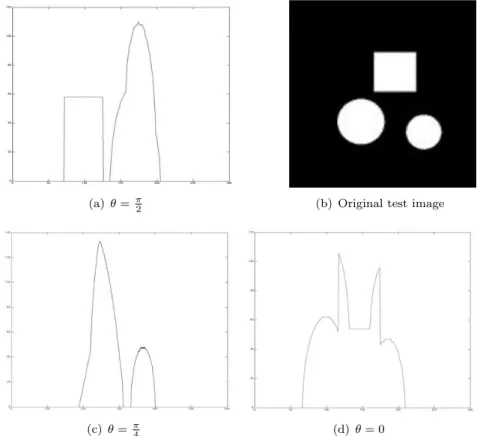
We consider an academic test object whose size is 256× 256 pixels. The different components are geometric objets with arbitrary uniform density. The (simulated) projection data are presented in next figure :
(a) θ = π2 (b) Original test image
(c) θ =π
4 (d) θ = 0
Figure 5.1. Test image and projection data
(a) Reconstruction with 18 views (b) Reconstruction with angles 0, π/4 and π/2 Figure 5.2. Reconstruction with filtered-back projection formula for data without noise (Ram-Lak filter with a Hann window and spline interpolation)
As expected the classical filtered-back projection gives very bad results because of the very few number of available data. Figure 5.2 presents the reconstruction with a Rak-Lam filter and a Hann window.
The tests have been performed using MATLAB�c. The prescribed tolerance εtol
is equal to 10−4 and Nmax = 2000. The accuracy for the conjugate gradient loop
5.2. Noiseless reconstruction
5.2.1. Sensitivity with respect to ε
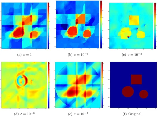
We first consider the case of noiseless data (which is unrealistic of course). The-oretically, the parameter ε should be chosen as small as possible, but the problem turns to be unstable (Aε is ill-conditioned) if ε is too small. The numerical results
for different values ε = 10−s, s = 0,· · · , 4 (see figure below) lead to the choice ε = 0.1 or ε = 0.01 .
(a) ε = 1 (b) ε = 10−1 (c) ε = 10−2
(d) ε = 10−3 (e) ε = 10−4 (f) Original
Figure 5.3. Noiseless data - sensitivity with respect to ε - τ = 15
(a) ε = 1 (b) ε = 10−1 (c) ε = 10−2 Figure 5.4. Noiseless data - sensitivity with respect to ε - τ = 15 - binary threshold : 0.5
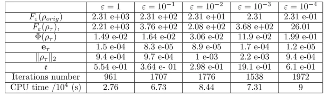
We call ρorig the original image and ρτ the computed solution. We report in
Table 5.2.1,
• Fε(ρorig) and Fε(ρτ),
• Φ(ρorig) and Φ(ρτ), the respective total variation
• the relative fitting data term eτ =
�
�H�k ρτ − πk�22
�πk�22
• the relative error :
e := �ρorig− ρτ�2 �ρorig�2
• the number of iterations, and
• the CPU-time. As we have not optimized the codes, the absolute CPU time makes no sense. We report here the CPU time to give a relative information.
ε = 1 ε = 10−1 ε = 10−2 ε = 10−3 ε = 10−4 Fε(ρorig) 2.31 e+03 2.31 e+02 2.31 e+01 2.31 2.31 e-01
Fε(ρτ), 2.21 e+03 3.76 e+02 2.08 e+02 3.68 e+02 26.01
Φ(ρτ) 1.49 e-02 1.64 e-02 3.06 e-02 11.9 e-02 1.99 e-01
eτ 1.5 e-04 8.3 e-05 8.9 e-05 1.7 e-04 1.2 e-05
�ρτ�2 9.4 e-04 9.7 e-04 1 e-03 2.2 e-03 9.4 e-04
e 5.54 e-01 3.64 e- 01 2.98 e-01 19.1 e-01 6.1 e-01 Iterations number 961 1707 1776 1538 1972 CPU time /104 (s) 2.76 6.73 8.44 7.31 9
Table 5.2.1. Sensitivity with respect to ε - Noiseless data - τ = 15 - Φ(ρorig) = 1.02e−02,��πk�22= 2.07e+06.
The above results clearly show the instability effects when ε is too small. 5.2.2. Sensitivity with respect to τ
We report the different errors in next table :
τ Fε(ρτ) Φ(ρτ) �ρτ�2 eτ e It. CPU time (s)
5 2.73 e+02 1.58 e-02 9.5 e-04 3.7 e-05 0.497 1570 6.21 e+04 15 3.76 e+02 1.64 e-02 9.75 e-04 8.27 e-05 0.365 1707 6.73 e+04 25 6.04 e+02 1.56 e-02 9.94 e-04 1.88 e-04 0.261 1587 6.65 e+04 35 7.56 e+02 2.09 e-02 9.82 e-04 2.64 e-04 0.317 1546 6.72 e+04 40 8.17 e+02 1.78e-02 9.87 e-04 2.92 e-04 0.284 2000 8.68 e+04 50 10.4 e+02 1.84 e-02 9.99 e-04 3.99 e-04 0.292 1583 6.8 e+04 60 11 e+02 1.80 e-02 9.9 e-04 3.8 e-04 0.275 1782 7.68 e+04 70 13.7 e+02 2.16 e-02 9.88 e-04 5.6 e-04 0.337 1676 7.19 e+04
Table 5.2.2. Sensitivity with respect to τ - Noiseless data - ε = 0.1 - Fε(ρorig) = 2.31e + 02 and Φ(ρorig) =
1.02e− 02.
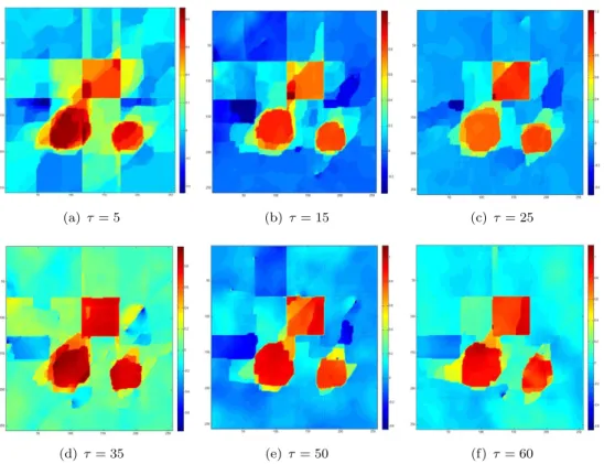
Figure 5.5 shows the solutions for ε = 0.1 and different values of the regulariza-tion parameter τ .
(a) τ = 5 (b) τ = 15 (c) τ = 25
(d) τ = 35 (e) τ = 50 (f) τ = 60 Figure 5.5. Noiseless data - ε = 0.1 - sensitivity with respect to τ
Figure 5.6. Noiseless data - ε = 0.1, τ = 25 - Normalized errors (Hk(ρτ)− πk)/max|πk| between the
projections of the solution and the (exact) data.
We note that the original object does not minimize the cost functional Fε, at
last for small τ . This comes from the modelling feature : the model we chose is not realistic enough. We have to look for another model that takes into account more accurately the physical context. Moreover, the best results are obtained with
small values of τ . This was predictable: in case the data are noiseless, the total variation penalization term is not useful (since there is no noise to remove). The total variation weight should quite small since the most important part of the functional F is the fitting data term.
We note that the reconstruction is not satisfying : we get an ellipse ( with a small excentricity parameter along the axis θ = π4 ) instead of a disk. Indeed such an object has projections very close to the ones of the original disk. It is hopeless to get a nice reconstruction without additional prior that allows to control this kind of perturbations. Other affects ( blur) are related to the large value of τ . In that case, the optimal solution is far from the original solution.
5.3. Case where data are noisy
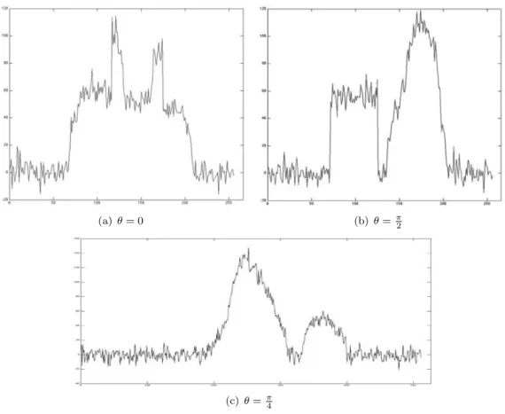
Now we consider noisy data: we have added to the “exact” (simulated) projection a gaussian white noise with standard deviation σ. We present results for σ = 0.05 (Figure 5.6).
(a) θ = 0 (b) θ = π2
(c) θ =π4
Figure 5.7. Noisy data - Gaussian noise with σ = 0.05
We report in next table the quantitative behaviour of the solutions. We have added the Signal to Noise Ratio, that we define here as
SN Rτ = log10 � i �Hiρτ�22 � i �Hi(ρτ− ρorig)�22 .
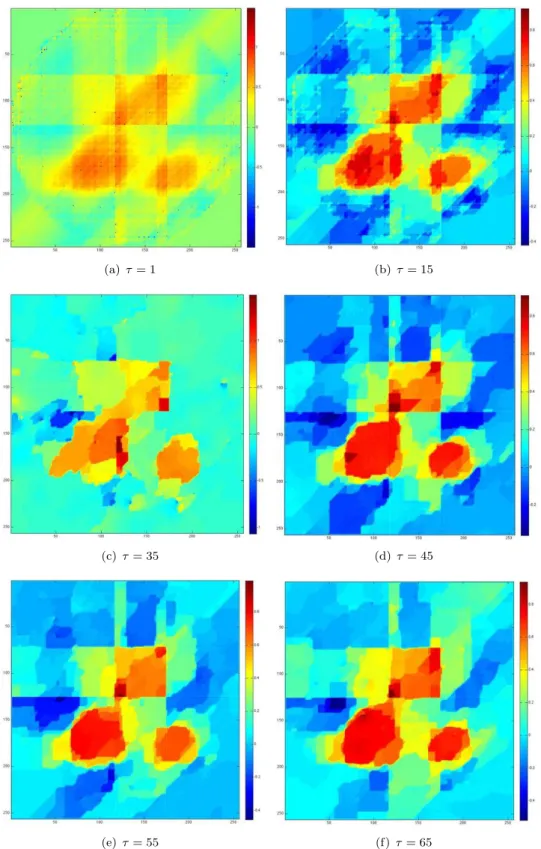
is measured via its projections. Next figure shows different solutions for ε = 1 and different τ values:
(a) τ = 1 (b) τ = 15
(c) τ = 35 (d) τ = 45
(e) τ = 55 (f) τ = 65 Figure 5.8. Reconstruction with noisy data - ε = 1 − σ = 0.05
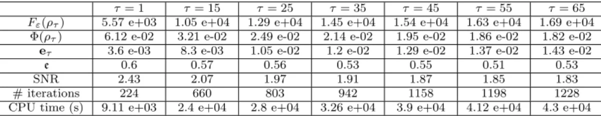
τ = 1 τ = 15 τ = 25 τ = 35 τ = 45 τ = 55 τ = 65 Fε(ρτ) 5.57 e+03 1.05 e+04 1.29 e+04 1.45 e+04 1.54 e+04 1.63 e+04 1.69 e+04
Φ(ρτ) 6.12 e-02 3.21 e-02 2.49 e-02 2.14 e-02 1.95 e-02 1.86 e-02 1.82 e-02
eτ 3.6 e-03 8.3 e-03 1.05 e-02 1.2 e-02 1.29 e-02 1.37 e-02 1.43 e-02
e 0.6 0.57 0.56 0.53 0.55 0.51 0.53 SNR 2.43 2.07 1.97 1.91 1.87 1.85 1.83 # iterations 224 660 803 942 1158 1198 1228 CPU time (s) 9.11 e+03 2.4 e+04 2.8 e+04 3.26 e+04 3.9 e+04 4.12 e+04 4.3 e+04 Table 5.3.1. Noisy data reconstruction (σ = 0.05) - ε = 1 - Sensitivity to τ - Fε(ρorig) = 2.07 e + 04, Φ(ρorig) =
1.02 1e− 02
Next figures show the projections of the computed object with respect to the observed (noisy) projections and to the exact one.
(a) Computed solution (continuous line) and noisy data (dotted line) - θ = 0
(b) Computed solution (continuous line) and exact data (dotted line) - θ = 0
(c) Computed solution (continuous line) and noisy data (dotted line)- θ = π
(d) Computed solution (continuous line) and exact data (dotted line) - θ = π
(e) Computed solution (continuous line) and noisy data (dotted line) - θ = π/2
(f) Computed solution (continuous line) and exact data (dotted line) - θ = π/2
Figure 5.9. Comparison between computed, observed and exact projections - σ = 0.05, ε = 1, τ = 55
(a) Solution - Threshold 0.5 (b) Original
Figure 5.10. Reconstruction with noisy data - ε = 1 − σ = 0.05 − τ = 55 - Thresholded solution (threshold =0.5)
The sensitivity to parameter τ is an important point. If τ is too small, we cannot get rid of the noise efficiently. If it is too large the computed solution is far from the (real) expected one. The parameter τ has to be related to the noise level. Next figure presents the evolution of SN Rτ with respect to τ for different values of σ
(a) SNR - σ = 0.1 (b) SNR - σ = 0.05 (c) SNR - σ = 0.01 Figure 5.11. SNR behavior with respect to τ and different σ, ε = 1 (dotted line) and ε = 0.1 (continuous line)
6. Conclusion
The variational model allows to get acceptable results for a severely ill posed prob-lem . However, the penalization term ε2�Lρ�2
2is not physically realistic if we choose
L = Id. The choice of L as high-pass or low-pass filter allows to add priors on the reconstructed object : we may decide to recover specific frequencies of the object . The numerical scheme has to be improved as well : the resolution of the linear system (4.21), Aεµ = b should be faster. It may be performed using a Choleski
decomposition of Aεif we get performant hardware. It should be interesting as well
to use a new efficient primal-dual algorithm [11] that is a good alternative to the Nesterov method.
At last, we need to add priors on the object to let the model more precise and realistic. In practise, the object is “almost” axisymmetric and could be recovered using a deformation from a symmetric one. One can recover a symmetric object from the available data with techniques of [1, 8] . Then we may look for a defor-mation vector field that drives the axisymmetric object to the non symmetric one. This point of view will be studied in a forthcoming work.
References
[1] R. Abraham, M. Bergounioux, and E. Tr´elat, A penalization approach for tomographic reconstruction of binary axially symmetric objects, Applied Mathematics and Optimization (2008), no. 58:345-371. [2] R. Acar and C.R. Vogel, Analysis of bounded variation penalty methods for ill-posed problems, Inverse
Problems 10 (1994), no. 6:1217–1229.
[3] L. Ambrosio, N. Fusco, and D. Pallara, Functions of bounded variation and free discontinuity prob-lems, Clarendon Press – Oxford, 2000.
[4] J.F. Aujol, Some first-order algorithms for total variation based image restoration, J Math Imaging Vis (2009), no. 34: 307-327.
[5] K.J. Batenburg, Reconstructing binary images from discrete x-rays, Tech. report, Leiden University, The Netherlands, 2004.
[6] , A network flow algorithm for binary image reconstruction from few projections, (2006), no. 4245:6–97.
[7] R.H.T. Bates, K.L. Garden, and T.M. Peters, Overview of computerized tomography with emphasis on future developments, Proeedings IEEE, vol. 71, 1983, pp. 256–297.
[8] M. Bergounioux and E. Tr´elat, A variational method using fractional order hilbert spaces for tomo-graphic reconstruction of blurred and noised binary images, Journal of Functional Analysis (2010), no. 259: 2296–2332.
[9] H. Br´ezis, Analyse fonctionnelle, th´eorie et aplications, Dunod-Masson, 1987.
[10] A. Chambolle, An algorithm for total variation minimization and applications, Journal of Mathe-matical Imaging and Vision (2004), no. 20:89–97.
[11] A. Chambolle and T. Pock, A first-order primal-dual algorithm for convex problems with applications to imaging, J. Math. Imaging Vision (2011), no. 40 (1):120–145.
[12] M. Courdurier, F. Noo, M. Defrise, and H. Kudo, Solving the interior problem of computed tomography using a priori knowledge, Inverse Problems (2008), no. 24.
[13] N.J. Dusaussoy, Image reconstruction from projections, SPIE’s international symposium on optics, imaging and instrumentation, San Diego, 1984.
[14] I. Ekeland and R. Temam, Convex analysis and variational problems, SIAM Classic in Applied Math-ematics, 28, 1999.
[15] G. Herman, Image reconstruction from projections: the fundamentals of computerized tomography, Academic Press, 1980.
[16] B. Hofmann, B. Kaltenbacher, C. P¨oschl, and O. Scherzer, A convergence rates result for tikhonov regularization in banach spaces with non-smooth operators, Inverse Problems (2007), no. 23:987–1010. [17] Y. L. Hstao, G.T. Herman, and T. Gabor, A coordinate ascent approach to tomographic reconstruction
of label images from a few projections, (2005), no. 151:184-197.
[18] , Discrete tomography withj a very few views, using gibbs priors and a marginal posterior mode approach, (2005), no. 20:399-418.
[19] J.-M.Dinten, Tomographie `a partir d’un nombre limit´e de projections : r´egularisation par des champs markoviens, Ph.D. thesis, Universit´e de Paris–Sud, 1990.
[20] A. Kirsch, An introduction to the mathematical theory of inverse problems, Springer-verlag, New York, 1996.
[21] F. Natterer, The mathematics of computerized tomography, SIAM, 2001.
[22] F. Natterer and F. W¨ubeling, Mathematical methods in image reconstruction, SIAM, 2001. [23] Y. Nesterov, Smooth minimization of non-smooth functions, Mathematic Programming, Ser. A
(2005), no. 103:127-152.
[24] F. Noo, R. Clackdoyle, and J.D. Pack, A two-step hilbert transform method for 2d image reconstruc-tion, Physics in Medicine and Biology (2004), no. 49(17):3903-3923.
[25] D. Partouche-Sebban and I. Abraham, Scintillateur pour dispositif d’imagerie, module scintillateur, dispositif d’imagerie avec un tel scintillateur et proc´ed´e de fabrication d’un scintillateur, French patent no 2922319, April 2009.
[26] D. Partouche-Sebban, I. Abraham, S. Lauriot, and C.Missault, Multi-mev flash radiography in shock physics experiments: Specific assemblages of monolithic scintillating crystals for use in ccd-based imagers, X-Ray Optics and Instrumentation (2010), Article ID 156984– 9p.
[27] E.T. Quinto, Singularities of the x-ray transform and limited data tomography in 2 and 3, SIAM
J. Math. Anal. (1993), no. 24:1215-1225.
[28] P. Weiss, G. Aubert, and L.Blanc-F´eraud, Efficient schemes for total variation minimization under constraints in image processing, SIAM Journal on Scientific Computing (2009), no. 31 (3):2047–2080.