HAL Id: hal-01790287
https://hal.archives-ouvertes.fr/hal-01790287
Submitted on 11 May 2018
HAL is a multi-disciplinary open access
archive for the deposit and dissemination of
sci-entific research documents, whether they are
pub-lished or not. The documents may come from
teaching and research institutions in France or
abroad, or from public or private research centers.
L’archive ouverte pluridisciplinaire HAL, est
destinée au dépôt et à la diffusion de documents
scientifiques de niveau recherche, publiés ou non,
émanant des établissements d’enseignement et de
recherche français ou étrangers, des laboratoires
publics ou privés.
Minimization of the Diffusion Delay of a Tree-Based
Wireless Sensor Network
François Delobel, Alexandre Guitton, Michel Misson, Waltenegus Dargie
To cite this version:
François Delobel, Alexandre Guitton, Michel Misson, Waltenegus Dargie. Minimization of the
Dif-fusion Delay of a Tree-Based Wireless Sensor Network. Globecom (IEEE Global Communications
Conference), 2011, Houston, Texas, United States. �hal-01790287�
Minimization of the Diffusion Delay of a
Tree-Based Wireless Sensor Network
Franc¸ois Delobel, Alexandre Guitton, Michel Misson
Clermont-Ferrand University, LIMOS CNRS Complexe scientifique des C´ezeaux
63177 Aubi`ere c´edex, France
Email:{delobel,guitton,misson}@sancy.univ-bpclermont.fr
Waltenegus Dargie
Chair for Computer Networks, Faculty of Computer Science Technical University of Dresden
01062 Dresden, Germany Email:{waltenegus.dargie}@tu-dresden.de
Abstract—In wireless sensor networks, saving energy is crucial
in order to increase the network lifetime. Energy is often saved by synchronizing the nodes activity, and having long periods of inactivity, or by having nodes exchange a global activity schedule. The synchronization and the exchange of a global schedule are two examples where information is broadcast from a specific node to the whole network. In this paper, we focus on the delay required to broadcast information in the whole network using a tree topology. We first show that the diffusion delay can be significantly reduced by utilizing the parallelization of node processing. We provide an exact algorithm in order to find optimal solutions. Then, we propose a linear algorithm that is able to find good solutions. We compare the exact solution to the heuristic solution on a workstation and conclude that our heuristic is very competitive and can be used to reduce the diffusion delay of a broadcast frame in a tree.
Keywords: wireless sensor network, synchronization delay,
diffusion delay, tree topology, transmission scheduling. I. INTRODUCTION
Wireless sensor networks (WSNs) are considered for a large variety of applications, including the monitoring of vast areas and military surveillance [1]. These networks are composed of small battery powered nodes which integrate a set of sensors, limited computational capabilities, a short-range communication module, and small-sized memory.
The main objective of a WSN is to monitor an external phenomenon for a long period of time. A critical issue is to reduce the energy used by the network protocols while being able to follow the evolution of the phenomenon. This is especially challenging as nodes spend about as much energy when listening (or receiving) than when transmitting [2], [3], [4]. Nodes have additional specificities compared to traditional computers. They often use a processor with limited computing capabilities, which yields to large processing times. Addition-ally, they are often based on a dual architecture (radio and processor) communicating through a SPI interface bus, which further increases the processing time.
In most WSNs, a global synchronization mechanism is often used to address the energy consumption issue, where nodes share a common temporal basis. Once nodes are synchronized, they can coordinate their activities, which helps reducing the energy used in several ways: (i) nodes can schedule their inactivity period so that they are all sleeping as much as
possible, (ii) nodes can minimize overhearing by listening only when a sender is transmitting, (iii) nodes can refrain from transmitting simultaneously, which reduces collisions. One way to achieve global synchronization is by broadcasting a beacon message on a tree structure. The beacon may contain global information about the schedules of the nodes.
In this paper, we minimize the time required to broadcast a message to all the nodes of a WSN. We show that the processing time has an important impact on the diffusion delay, and we propose algorithms to reduce it. Our solution is generic and can be applied in order to broadcast an information, or to minimize the synchronization time. Reducing the synchro-nization time is crucial as it is an overhead for the nodes: the shorter the synchronization, the less energy is spent.
The remaining of the paper is structured as follows. In Sect. II, we characterize the diffusion delay on nodes and we formally describe the problem of minimizing the diffusion delay. In Sect. III, we present two exact solutions for the problem: with an integer linear program and with a Branch-and-Bound method. In Sect. IV, we propose an approximation which runs in a linear time with respect to the number of nodes in the network. This algorithm is implemented on a real platform. We conclude our work in Sect. V.
II. PROBLEM DESCRIPTION
Several protocols in WSNs are based on a tree topology, since it is easy to maintain when nodes mobility is low. Several synchronization protocols for WSN are described in [5].
The RBS protocol (Reference Broadcast Synchroniza-tion [6]) is a tree-based, receiver-to-receiver synchronizaSynchroniza-tion protocol. The authors of RBS show that the time between the transmission of a message and the reception of the message is subject to a random delay, due to random access mechanisms or an unpredictable processing time. The synchronization in RBS is only performed among receivers, and not with the sender of a message. This approach eliminates uncertainties due to random delays at the sender compared with traditional sender-to-receiver synchronization protocols.
The TPSN protocol (Timing-sync Protocol for Sensor Net-works [7]) is a tree-based, sender-to-receiver synchronization protocol. Nodes in TPSN are activated sequentially, depending on their depth on the tree. Nodes in TPSN estimate the clock
drift using a handshake procedure with their parent. The main advantage of TPSN over RBS is that it consumes less energy, at the cost of a reduced accuracy.
The IEEE 802.15.4 standard [8] defines the lower layers of a low power wireless personal area network (LP-WPAN). The ZigBee standard [9] defines the upper layer of a LP-WPAN, and assumes that the lower layers operate IEEE 802.15.4. In ZigBee, nodes are either coordinators or end-devices. The nodes form a tree topology called the cluster-tree, where end-devices are leaves, coordinators are internal nodes, and the root is a special coordinator called the PAN (personal area network) coordinator. In the subsequent parts, we use the ZigBee definitions of coordinators and end-devices.
In this paper, we make the following assumptions: the PAN coordinators knows the tree topology, the diffusion is based on a master-slave multi-hop approach. The first assumption is common in ZigBee or in Wireless HART for instance: the network manager has the knowledge of the logical structure of the topology. The second assumption is the same as in [7], [10]: the synchronization is scheduled by the PAN coordinator.
A. Diffusion delay of a broadcast frame
Synchronization protocols (or, more generally, diffusion protocols) are often based on a sequence of broadcasting. The interval between two broadcasts depends mostly on the processing time and on the architecture of the node. Indeed, most existing nodes are built according to a dual architecture: a radio module (e.g. a CC2420 component [2]) and a processor (usually operating at 4 MHz or 8 MHz), interconnected through a SPI interface at 500 kbps. As the commonly used physical layer of IEEE 802.15.4 is operated at 250 kbps, the time required to transmit a frame through the SPI interface is half the time required to transmit the frame in the medium. The processing time, the possible SPI communication time, and the transmission time have significant impacts on the overall diffusion delay of a broadcast frame.
To compute the diffusion delay of a broadcast frame, we assume that the frame is broadcast in a multi-hop manner by all the coordinators of the network. As end-devices can only receive from their designated parent, all the coordinators of the network have to transmit. For simplicity reasons, we do not show in the rest of this paper the end-devices.
We assume that nodes transmit the broadcast frames se-quentially. This guarantees that there is no collision between frames, which would dramatically increase the delay. Allow-ing distant nodes to transmit simultaneously is an issue in WSNs [11], as the location of nodes is often unknown and propagation conditions may vary due to the mobility of nodes. The PAN coordinator computes a sequence containing all the coordinators of the network, and includes it in the diffusion frame. Then, it broadcasts the frame. When a coordinator n receives the diffusion frame from a node s, it determines the current relative time from the location of s in the sequence. Then, it computes its own transmission time based on the
number of nodes between s and n in the sequence1.
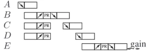
Figure 1 shows an example topology of five nodes: node A is the PAN coordinator, and the other four nodes are coordinators. These coordinators have end-devices attached to them. Figure 2 describes how time is spent by nodes during the diffusion of a frame, when the sequence is(A, B, C, D, E) and the topology is the one given in Fig. 1. First, A builds the frame in the main processing module and sends it to its radio module through the SPI interface, which is depicted as a box with an arrow. Then, A transmits the frame. The frame is simultaneously received by B, C and D (the time of flight being negligible in WSNs). The radio modules of each of these coordinators send the frame to the processing module (which is depicted as a box with an arrow) and they all process it (which is depicted as a box with PR). Coordinator B detects that it directly follows A in the sequence, and transmits the frame to its radio module. During this time, coordinators C and D are waiting (or sleeping if there is enough time). Coordinator C wakes up after B has completed the transmission2. The process goes on until all the coordinators have sent the frame. Note that in the figure, we set the transmission time on the SPI interface to half the time of the transmission on the channel. We also assumed a small processing time PR, which might not be the case in practice.
A
B C D
E
Figure 1. An example topology for the diffusion.
PR PR PR PR A B C D E time
Figure 2. Non-optimized diffusion delay for a given sequence.
PR PR PR PR A B C D E gain
Figure 3. Optimized diffusion delay for a given sequence.
Because the time required to send a frame from the process-ing module to the radio module is known (it depends only on
1The transmission duration is not the same for each node. In this paper,
we assume that n can be determined from the sequence itself.
2Again, we assume here that C knows the time B is going to spend
the bandwidth of the SPI interface and on the length of the frame), coordinators can send the frame in advance. In the previous example, coordinator C can wake up a short time before B completes the transmission, and C can start sending the frame to the radio module. Figure 3 shows an optimized version of the diffusion, with a gain at coordinators C and D. Let us give a numerical estimation of the different times involved. The transmission of a medium-sized frame of 50 bytes on the wireless channel is performed at 250 kbps. Thus, it takes about 1.6 ms. The transmission of the frame on the SPI interface takes about 0.8 ms. The processing time of a frame takes about 1 ms when only basic operations are performed.
B. Optimization of the diffusion delay
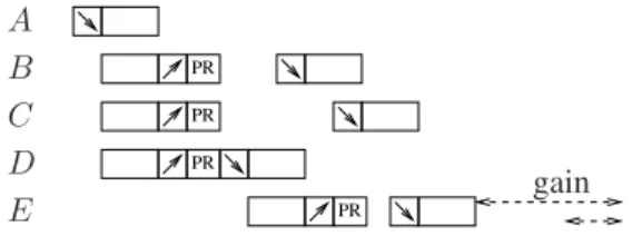
It can be understood from the previous example that the medium is unused during a short time between the trans-mission of coordinators D and E. When E receives the frame from D, it has to process it. Then, it detects that it directly follows D in the order and send the frame as soon as possible. If a coordinator X had been between D and E in the order, the processing time of E would not have increased the diffusion delay, as E would have processed the frame during the transmission time of X.
Figure 4 shows the diffusion delay of the topology of Fig. 1, using the sequence (A, D, B, C, E). Notice that, in this sequence, E does not directly follow D. The reduction of the diffusion delay is very important compared to the initial sequence, due to the parallelization of the activities. While E processes the message, other coordinators are using the channel. The proposed sequence is optimal.
PR PR PR PR A B C D E gain
Figure 4. Optimized diffusion delay for an optimal sequence.
C. Model and definitions
In this paper, we study how to build an optimal sequence for the diffusion of a frame, given a tree.
Let T be a tree representing a WSN, where N is a set of |N | = n nodes. Let ~o(T ) be a sequence on T , representing the order of emission of the node. In the remaining part of the paper, we call ~o(T ) an order. As each node needs to wait for a beacon before being able to transmit, ~o(T ) has to be a
topologicalorder. We use the following notations. f ather(n) is the node n′ such that n′ is the father of n in(T ), pred(x) (resp. succ(d)) is the node before (resp. after) x in an order ~
o(T ), and f irst(d) (resp. last(d)) is the first (resp. last) node of depth d that appears in ~o(T ).
Previously, we showed that the occurrence of a child directly after its father in an order has a negative impact on the delay. We call this situation a conflict. For a topological order ~o(T )
and a node x, we define the predicate conf lict(x) which is true if and only if pred(x) = f ather(x). A conflict in an order ~o(T ) for a node x is represented by underlining x.
The diffusion delay depends on the number of nodes in the network, and on the number of conflicts. As the number of nodes in the network is fixed, we define the duration of an order ~o(T ) as the number of nodes x in T for which conf lict(x) is true. We use the notation d(~o(T )) to denote the number of conflicts in an order ~o(T ).
Note that a depth-first order of T yields a longer duration than a breadth-first order of T . In the following, we consider that a breadth-first order is a good solution.
III. EXACT SOLUTION
We propose in this section two algorithms in order to obtain exact solutions. The first uses integer linear programming. The second is a Branch-and-Bound algorithm.
A. Integer linear programming
A way to compute an optimal order ~o(T ) for a tree T is to define an integer linear program. The algorithm uses a set of m nodes denoted by N . A set P is used to represent the positions of the nodes in an order.
We also define the following relations. pos(n) represents the position of a node n in an order. permut(n, p) is a boolean matrix which describes the position p of a node n in an order. δ(n1, n2) is m plus the difference in the position of nodes n1 and n2 in an order. The addition of m ensures that δ(n1, n2) ≥ 0, which is required later on (see Subsect. III-A2). conflict(n) indicates whether node n directly follows its father in the order, which induces a conflict, or not. Finally, the real variables λi and the binary variables xi are used in order to model conflicts (see Subsect. III-A2). Note that our modelization uses mixed integer linear programming due to the requirement of the variables λi to be real.
1) Modelling of the constraints: We use the following variables in our mixed integer linear program. pos(n) is the position of n in the order (in {1, . . . , P }). permut(n, p) indicates whether n is at position p or not (in{0, 1}). δ(n1, n2) is the difference of positions of nodes n1 and n2 in the order, plus m (in{0, . . . , 2m}). conflict(n) indicates whether n directly follows its father in the order or not ({0, 1}). λi(n) is in IR+
and xi(n) is in {0, 1}.
Constraints 1 and 2 in Table I ensure that the order is a permutation of nodes (through the use of permut(n, p)). Constraint 3 maps each node n to its position pos(n) in the order, while Constraint 4 ensures that the order is topological. Finally, Constraint 5 attributes the correct value to δ(n1, n2).
2) Modelling of the conflict(n) constraint: Constraints 6 to 12 are used to model conflicts. Recall that a conflict occurs for a node n if and only if n directly follows its father in the order. This means that the difference between pos(father(n)) and pos(n) is equal to 1. Thus, if we denote by d(n) the difference of positions between n and father(n) in the order, we can define conflict(n) in the following way: conflict(n) = 1 if
MinimizeP
n∈Nconflict(n) such that:
(1)∀n ∈ N ,P p∈Ppermut(n, p) = 1 (2)∀p ∈ P ,P n∈Npermut(n, p) = 1 (3)∀n ∈ N , pos(n) =P p∈P(p · permut(n, p)) (4)∀n ∈ N , pos(n) ≥ pos(father(n)) (5)∀n1, n2∈ N2, δ(n1, n2) = pos(n1) − pos(n2) + m (6)∀n ∈ N , conflict(n) = λ3(n) (7)∀n ∈ N , δ(n, father(n)) = mλ2(n)+(m+1)λ3(n)+(m+2)λ4(n)+ 2mλ5(n) (8)∀n ∈ N , λ1(n) ≤ x1(n) (9)∀n ∈ N , ∀i ∈ {2, 3, 4}, λi(n) ≤ xi−1(n) + xi(n) (10)∀n ∈ N , λ5(n) ≤ x4(n) (11)∀n ∈ N ,P i∈{1,2,3,4}xi(n) = 1 (12)∀n ∈ N ,P i∈{1,2,3,4,5}λi(n) = 1 Table I
CONSTRAINTS OF THE MIXED INTEGER LINEAR PROGRAM.
d(n) = 1, and 0 otherwise. Unfortunately, conflict(n) is not a convex function of d(n).
conflict(n) can be defined as a step function of a positive variable δ(n), with δ(n) = d(n)+m. Formally, conflict(n) can be defined in the following way. Let a1 = 0, a2= m, a3= m+ 1, a4 = m + 2 and a5= 2m, and conflict(n)(a1) = 0, conflict(n)(a2) = 0, conflict(n)(a3) = 1, conflict(n)(a4) = 0 and conflict(n)(a5) = 0. Such a formulation can be used to model conflict(n) using mixed integer linear programming, as described in Ineq. 4.18 of [12] (notice that a1 has to be greater than or equal to 0, and thus our addition of m in δ(n)). Constraints 6 to 12 follow from this formulation.
The integer linear program described in the previous subsec-tion is computasubsec-tionally expensive. Some instances of twenty nodes are solved in several hours by a workstation using GLPK (GNU Linear Programming Kit). Indeed, the modelization of the conflicts and the number of integer variables make the problem hard to solve. Thus, we decided to implement a Branch-and-Bound algorithm to find exact solutions quickly.
B. Branch-and-Bound algorithm
A Branch-and-Bound algorithm [13] finds an optimal solu-tion by exploring a treeT of all possible solutions. The quality of each solution is computed while exploring the tree. If the algorithm determines that all the solutions in a sub-tree have a lower quality than an existing solution, the algorithm stops the evaluation of the sub-tree, thus saving processing time. Therefore, the efficiency of a Branch-and-Bound algorithm comes from two criteria: (i) the quality of the initial solution, and (ii) the relationship between the quality of a solution s∈ T and the quality of the solutions in the sub-tree of s.
The treeT explored by the Branch-and-Bound algorithm is an n-ary tree. T is built in the following way. Each node of the tree is an order. The root is the empty order. If a node of T is an order o of k nodes, it has n − k children in T . The i-th child is the order o· ni, where ni is the i-th node of N not present in on. TreeT has n! leaves, which are all the possible orders of the n nodes. Not all the possible orders are valid (as some of them are not topological), but the optimal order is one of the leaf of T .
The topological rule ensures that orders that are not topo-logical are not examined, as they cannot correspond to a valid solution. The branching rule assumes that the best current solution (possibly not optimal) is known and cuts subtrees of T whose duration is larger than the current best. The key here is that the duration of an order on is always smaller than or equal to the duration of any topological order on· ni.
The choice of the initial reference solution is crucial. We used our heuristic described in Sect. IV as an initial solution. Breadth-First algorithm (BF) is compared to the optimal so-lution (computed with Branch-and-Bound) using two topolo-gies: random trees and interconnection of random hot-spots.
1) Random trees: Random trees are designed to model interconnections between nodes in a dense WSN. Nodes are added to the tree one by one. They are attached to any existing node of the tree, except to those having already more than Rm children. Note that this limitation is consistent with the cluster-tree topology formation of ZigBee [9]. The location of nodes are not generated by this algorithm, because only tree structures have an impact on the order duration. With this tree generation algorithm, trees tend to become complete rather than grow deeper.
In our simulations, we used Rm= 5. We varied the number of nodes from 50 to 2000. For each number of nodes, we generated 1000 trees. Generating all the trees and finding the optimal solution using the Branch-and-Bound algorithm takes about half an hour on an i7 930 workstation.
The percentage of trees where the breadth-first order was not optimal, varies between 15% and 21.1% (on average 17.9% with a standard deviation of 1.35). It does not depend on the number of nodes (from node numbers varying from 50 to 2000). The average duration of breadth-first orders, when they are not optimal, is on average about 2.17 (while the optimal duration is on average 1) with a standard deviation of 0.03. These results do not change as the number of nodes vary. Consequently, breadth-first orders are good approximations of the optimal order when random trees are generated.
2) Interconnection of random hot-spots: When the network is dense, it is possible to find optimal solutions having a very low duration. We consider here a network constituted of two hot-spots, interconnected by a chain of nodes. The root of the tree is located in one of the hot-spot3. The generator first places x nodes with sensors within the hot-spots, then adds as many nodes as required in order to build a tree in each hot-spot, and interconnects the two hot-spots by deploying a chain of nodes. The generated tree includes only the non sensor nodes.
The topologies were generated using the following parame-ters. The communication range of nodes is about 15 m. Each hot-spot has a diameter of40+x
2 m, and consists of x sensors. The distance between the two hot-spots is about8 ∗ x m. The coordinator is added to the center of one hot-spot. We varied x from 5 to 20, and we generated 100 trees for each x. Note
3Such a topology is a worst-case scenario for the duration of the order.
Indeed, when a tree possesses a single, sufficiently long chain of nodes, all topological orders contain the nodes of the chain in sequence, and the optimal duration increases significantly.
that the number of nodes n depends on x. Note that with the trees generated, the breadth-first order duration is usually far away from the optimal duration, which causes the Branch-and-Bound algorithm to take hours to solve instances of 60 nodes.
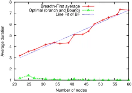
Figure 5 shows the average duration of Breadth-First and optimal orders, as x varies. It can be seen that the duration of the breadth-first order grows proportional to x, as hot-spots are separated by a distance proportional to x. Variations in the breadth-first duration are due to different tree topologies. The optimal order yields a duration of 1 conflict on average, which means that the nodes of the first hot-spot are used by the optimal order to break the chain of nodes. If the two hot-spots were separated by a larger distance (for instance, if the distance between the hot-spots would exceed15x), the optimal duration could not be equal to 1.
1 2 3 4 5 6 7 8 20 25 30 35 40 45 50 55 60 Average duration Number of nodes Breadth-First average Optimal (branch and Bound) Line Fit of BF
Figure 5. Average duration of breadth-first and optimal orders, for intercon-nections of hot-spots.
IV. HEURISTIC METHOD
In this section, we present an algorithm that approximates the optimal order in linear time. The general idea for this algorithm is to improve a breadth-first order by permuting and moving nodes in the order without changing the tree topology.
A. Permuted order
Let us consider a breadth-first order. Such an order can cause at most one conflict per depth d. If there is a conflict at depth d, we apply one of the three permutation rules. Permutation P1 is applied if and only if there are at least three nodes on depth d. Permutation P1 consists in swapping succ(f irst(d)) and last(d) in the current order. Figure 6 shows Permutation P1 applied on an example. Permutation P2 is applied if and only if (i) there are exactly two nodes on depth d and (ii) f irst(d) and last(d) have the same father. Permutation P2 consists in swapping f irst(d) and last(d) in the current order. Permutation P3 is applied if and only if (i) there are exactly two nodes on depth d and (i) f irst(d) and last(d) have a different father. Permutation P3 consists in swapping f irst(i) and last(i) for each depth i such that (i) j < i≤ p, (ii) there are exactly two nodes on depth i that have a different father and (iii) at depth j, there is either one node, two nodes with the same father or three or more nodes. If there are two nodes at depth j, they are swapped. If there are three or more nodes at depth j, a node nxj that is neither
the father of f irst(j + 1) nor of last(j + 1) is swapped with node last(j). Figure 7 shows Permutation P3 applied on an example. A permuted order P(T ) can be computed by first considering permutations P1 and P2 from depth 1 to h, and then considering permutations P3 from depths1 to h.
A A
B C D D C B
E E
⇒
ABCDE⇒ ADCBE
Figure 6. Permutation P1 reduces by one the duration of the order.
A A C C B B D D E E F F G G H H I I ⇒
ABCDEF GHI ⇒ ADCBF EHGI
Figure 7. Permutation P3 reduces by one the duration of the order.
B. Displaced order
The displaced order enhances the permuted order by remov-ing the constraint of havremov-ing nodes sorted by depths. Let ~o(T ) be a topological order. If last(d) is the father of f irst(d + 1) in ~o(T ), and if depth d contains only one node last(d), the displaced order moves an available node for last(d) between last(d) and f irst(d+1). A node nxis said to be available for a node last(d) if it satisfies the following conditions: (i) nxis directly preceded by node na and directly followed by node nb, (ii) nxhas no child in the tree T (so that the order remains topological), (iii) nx is before last(d) in the order ~o(T ), and (iv) either na is the father of nxand of nb, or nais the father of neither nx nor of nb. Figure 8 shows an example of a displaced order, where the available node is B. A displaced
order D(T ) is computed by considering displacements from depths1 to h. Our heuristic consists in building D(T ).
A A B B C C D D ⇒ E E A0 B1 AC 1 AD 2 CE 3 D⇒ A 0 C1 AD 2 CB 1 AE 3 D
The computation of D(T ) is realistic for real nodes, as it only requires a time which is a linear function of n, as follows. The breadth-first order B(T ) can be computed in O(n + m), where n is the number of nodes of T and m is the number of edges of T . As T is a tree, m= n − 1. Thus, B(T ) can be computed in O(n). The (potential) application of permutations P1 and P2 at each depth requires O(h). The (potential) application of permutations P3 at each depth also requires O(h): although P3 considers swapping nodes at previous depths, it is not possible for the same node to be considered twice. The overall complexity for P(T ) is O(n + h) = O(n).
The setD of all the available nodes, with respect to the last node of P(T ), can be computed in O(n). When the algorithm searches for an available node for last(d), only the first node ofD, denoted nx, needs to be considered. If nxis not available for last(d), this means that no further nodes in D are available for last(d). If nxis available,D has to be updated. As nxhas no children in T (due to the second constraint of the available nodes), the changes in D are limited to na and nb, which are the neighbor nodes of nx. In other words, once setD is computed (in linear time), it only decreases (in constant time). Thus, computing D(T ) requires O(n).
C. Simulation results
In this section, we study the performance of our heuristic with respect to breadth-first and and optimal approaches.
With the same random trees as previously, less than 0.8% of heuristic solutions are not optimal (on average 0.25% with standard deviation 0.16%). Note that heuristic solutions are at least as good as breadth-first solutions.
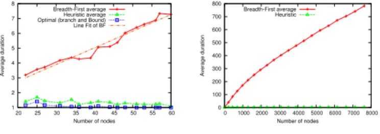
Figure 9 depicts the average duration of breadth-first, heuris-tic and optimal orders on small interconnected hot-spots. The figure shows that the heuristic improves greatly the duration of the breadth-first order, keeping the duration constant and close to the duration of the optimal solution. Figure 10 depicts the average duration of breadth-first and heuristic orders on large interconnected hot-spots, where the number of sensors varies from 0 to 2000, and 1000 instances are generated per size. We were not able to run the Branch-and-Bound algorithm on such topologies. The duration of the heuristic order remains nearly constant (most of the conflicts of the breadth-first orders can be repaired), whereas the duration of the breadth-first order grows proportionally with the number of nodes.
1 2 3 4 5 6 7 8 20 25 30 35 40 45 50 55 60 Average duration Number of nodes Breadth-First average Heuristic average Optimal (branch and Bound) Line Fit of BF
Figure 9. Average duration of breadth-first, heuristic and optimal orders, on small interconnected hot-spot trees. 0 100 200 300 400 500 600 700 800 0 1000 2000 3000 4000 5000 6000 7000 8000 Average duration Number of nodes Breadth-First average Heuristic
Figure 10. Average duration of breadth-first and heuristic orders, on large interconnected hot-spot trees.
V. CONCLUSION
Several protocols developed for WSNs require the diffusion of information in the whole network in a guaranteed manner. In this paper, we study the delay required to propagate the information to all nodes. We show that the order in which nodes transmit the data has a critical impact on the overall delay. Consequently, we propose two exact algorithms and a heuristic one in order to reduce the diffusion delay. Sim-ulations are performed on randomly generated trees and on randomly generated interconnection of hot-spots. We show that our heuristic is applicable in real scenarios and that it leads to near-optimal diffusion delays.
In a future work, we plan to adapt our study to graphs. We aim at finding the optimal diffusion order when the complete communication graph is given, rather than when a tree is given. We also plan to implement our heuristic on TelosB nodes in order to check the computation cost and memory requirements for relatively large networks.
REFERENCES
[1] I. F. Akyildiz, W. Su, Y. Sankarasubramaniam, and E. Cayirci, “Wireless sensor networks: a survey,” Computer networks, vol. 38, no. 4, 2001. [2] “CC2420 - 2.4 GHz IEEE 802.15.4 / ZigBee-ready RF Transceiver,”
Chipcon, preliminary datasheet, 2004.
[3] J. Elson and K. R¨omer, “Wireless sensor networks: A new regime for time synchronization,” in Hot Topics in Networks, 2002.
[4] J. Rahm´e, N. Fourty, K. Al Agha, and A. Van Den Bossche, “A recursive battery model for nodes lifetime estimation in wireless sensor networks,” in IEEE Wireless Communications and Networking Conference, 2010. [5] B. Sundararaman, U. Buy, and A. D. Kshemkalyani, “Clock
synchro-nization in wireless sensor networks: A survey,” Ad-Hoc Networks, vol. 3, no. 3, pp. 281–323, 2005.
[6] J. Elson, L. Girod, and D. Estrin, “Fine-grained network time synchro-nization using reference broadcasts,” in OSDI, December 2002. [7] S. Ganeriwal, R. Kumar, and M. B. Srivastava, “Timing-sync protocol
for sensor networks,” in ACM SenSys, 2003, pp. 138–149.
[8] IEEE 802.15, “Part 15.4: Wireless medium access control (MAC) and physical layer (PHY) specifications for low-rate wireless personal area networks (WPANs),” ANSI/IEEE, Standard 802.15.4 R2006, 2006. [9] ZigBee, “ZigBee Specification,” ZigBee Standards Organization,
Stan-dard ZigBee 053474r17, January 2008.
[10] M. Mock, R. Frings, E. Nett, and S. Trikaliotis, “Continuous clock synchronization in wireless real-time applications,” in IEEE SRDS, 2000, pp. 125–133.
[11] X. Wang, “Spatial channel reuse in wireless sensor networks,” Wireless
Networks, vol. 14, no. 2, pp. 133–146, 2008. [12] A. Billionnet, Optimisation discr`ete. Dunod, 2007.
[13] A. H. Land and A. G. D. Doig, “An automatic method of solving discrete programming problems,” Econometrica, vol. 28, no. 3, pp. 497–520, 1960.