A design for a high energy X-ray computed tomography sensor for the study of solidification fronts in aluminum

A Design for a High Energy X-Ray Computed Tomography

Sensor for the Study of Solidification Fronts in Aluminum

by

Imad Maurice Jureidini

B.S., Applied Physics, Columbia University, 1994

SUBMITTED TO THE DEPARTMENT OF NUCLEAR ENGINEERING IN PARTIAL FULFILLMENT OF THE REQUIREMENTS FOR THE DEGREE OF

MASTER OF SCIENCE IN NUCLEAR ENGINEERING AT THE

MASSACHUSETTS INSTITUTE OF TECHNOLOGY February 1997

@ 1997 Massachusetts Institute of Technology

All rights Reserved

Signature of Author:

'I

January 17, 1997

Certified by:

Research

Richard Lanza Scientist, Nuclear Engineering Department Thesis Supervisor Certified by:

Lawrence Lidsky Professor of Nuclear Engineering Thesis Reader Accepted by:

/Chiman,

/

/ Professor of Nuclear Engineering

Department Committee on Graduate Students

MAY

191997

A Design for a High Energy X-Ray Computed Tomography Sensor for the

Study of Solidification Fronts in Aluminum

by Imad Jureidini

Submitted to the Department of Nuclear Engineering

on January 17, 1997 in Partial Fulfillment of the Requirements for the Degree of Master of Science in Nuclear Engineering

ABSTRACT

CastScan, a computed tomography sensor, has been designed to study the solidification front of aluminum in a laboratory environment. The characteristics of this scanner are presented, along with the motivations behind its design and its expected performance.

X-ray computed tomography systems allow one to obtain two-dimensional, cross-sectional images of the density within a scanned sample. Liquid and solid metals vary in density by a few percent, making them a potential object of CT study. Because of the high density of metals, traditional low-energy CT systems such as those used in medicine are not useful. CastScan uses a 6 MeV electron linac to produces an intense beam of highly energetic, highly penetrative x-ray photons. To detect these photons, the system uses 120 channels of high density cadmium tungstate scintillation crystals coupled to silicon photodiodes. An aluminum sample is melted in a cylindrical furnace that resides on a computer controlled rotary and translational stage. The temperature of the sample is measured at 16 positions. A computer system allows the remote operation of the sensor from outside a shielded facility.

The CastScan system is expected to be capable of yielding images of the density of the aluminum sample within a 1.2 cm thick slab and with a maximum resolution of 1.1 mm, in a time on the order of one to a few minutes. This capability will allow the operator to resolve the profile of the solidification front within the aluminum sample. This system opens the possibility of real-time monitoring of the solidification front of metals in an industrial environment.

Thesis Advisor: Richard Lanza Title: Principal Research Scientist

Acknowledgments

I would like to thank Dr. Richard Lanza for introducing me to this project and for his guidance and advice over the past year. My thanks also go to Prof. Jung-Hoon Chun and Dr. Nanrlaji Saka. The three of them are the backbone of this project and allow it to be an ongoing success.

I am grateful to have such great colleagues and friends as my fellow graduate students Mark Hytros and DongSik Kim, who are not a bunch of freaks, even though they may think so. My gratitude goes to our undergraduate branch, Eric Empey.

I would like to thank Jeff DiTullio of the MIT Manufacturing Institute, as well as Dr. Tim Roney and Dr. Dennis Kunerth of the Idaho National Engineering Laboratory. The staff at the Bates Linear Accelerator Center, and particularly Kenneth Hatch, have proven invaluable to the advancement of our project. I would also like to thank our partners at Analogic Corporation, in particular John Dobbs and Hans Weedon, for their

commitment and efforts at providing us a detector system. Finally, I extend my

appreciation to Russ Schonberg and the folks at Schonberg corporation for their willingness to help and their friendliness.

This work was in part funded by the National Science Foundation (Grant No.

DMI-9522973) and the Idaho National Engineering Laboratory - University Research

Table of Contents

2. X-RAY COMPUTED TOMOGRAPHY .... ... 15

2.1. Photon Interactions ... ... 15

2.1.1. Photoelectric A bsorption ... 15

2.1.2. Compton Scattering... 16

2.1.3. Pair Production ... ... 19

2.2. Photon Attenuation ... 20

2.3. Principles of Computed Tomography ... ... 25

2.3.1. The Radon Transform ... 26

2.3.2. The Inverse Radon Transform ... ... 28

2.4. Photon Energy Requirem ents ... 31

3. X-RAY SOURCE: THE LINAC... 33

3.1. Principles of the L inac ... ... 33

3.1.1. Electron Acceleration in Linacs ... ... 34

3.1.2. Brem sstrahlung Radiation ... 37

3.2. Characteristics of MINAC 6 ... 39

3.2.1. Physical Characteristics... 39

3.2.2. Operating Characteristics ... 40

3.2.3. X-Ray Beam Characteristics ... ... ... 42

4. SOLIDIFICATION FRONT ... 46

4.1. Furnace and Cooling System ... 46

4.2. M otion system... 49

5. DETECTOR SYSTEM ... ... 50

5.1. Principles of X-Ray Detection ... 50

5.1.1. Gas-filled Cham bers... ₅₀

5.1.2. Scintillation ... ... 51

5.1.3. Photomultiplier Tubes and Photodiodes ... 54

5.1.4. X-ray detection for CT ... 55

5.2. Experimental Detection System ... 56

5.3. Scatter and Collimation ... ₅₇

5.3. 1. Detector Angular Sensitivity Characterization ... ... 57

5.3.2. Scatter Discrimination Properties... ... 60

6. FACILITY DESIGN ... 67

6.1. Experiment Layout... ₆₇

6.2. Shielding and Room Design ... 69

7. DATA AND SOFTW ARE ... ₇₂

7.1. Controls and Sensors ... 72

7.2. Control Environment ... ₇₃

8. PERFORM ANCE GOALS ... 76

8. 1. Resolution ... 76

8.2. Imaging Time.... ... ... ... ... 80

8.3. Dynamic Range ... . ... 84

9. CONCLUSIONS AND FUTURE WORK ... 85

9.2. A Priori Inform ation ... 86

9.3. Incomplete Data Sets and Limited Angle Tomography... 86

APPENDIX A. MINAC 6 Spectrum Computation -MCNP Code ... 87

APPENDIX B. Scatter Function Computation -MCNP Code ... 88

APPENDIX C. Resolution Calculation -IDL Code ... 98

APPENDIX D. Shielding Computation -MCNP Input Code ... 100

List of Tables

Table 1.1. Density variation between solid and liquid steel, aluminum and tin ... 13

Table 3.1. Components of the MINAC 6 linear accelerator... ... 39

List of Figures

Figure 1.1. Schematic of a continuous casting facility... 12

Figure 2.1. Schematic of the Compton scattering process ... 17

Figure 2.2. Energy of Compton scattered photons as function of the scatter angle ... 18

Figure 2.3. Polar plots of the probability of Compton scattering as a function of the scattering angle 0 for a variety of photon energies ... 19

Figure 2.4. Schematic of the pair production process ... 20

Figure 2.5. Linear attenuation coefficients for aluminum for photon energies ranging from 10 keV to 100 MeV ... ... 23

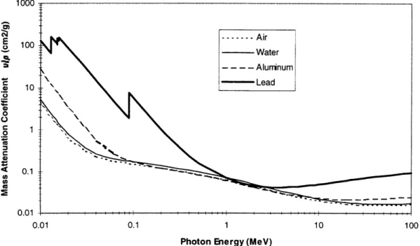
Figure 2.6. Mass attenuation coefficients of air, water, aluminum and lead as a function of photon energy ... 24

Figure 2.7. Schematic of a radiography experiment... 25

Figure 2.8. Radon transform geom etry... 27

Figure 2.9. Sample bitmap (left) and its corresponding sinogram (right) ... 28

Figure 2.10. Filtered backprojection of a sample sinogram (left) and unfiltered backprojection of the same sinogram (right) ... 30

Figure 3.1. Time evolution of the longitudinal electric field in a traveling wave linac ... . . ... 35

Figure 3.2. Time evolution of the longitudinal electric field in a standing wave linac ... 36

Figure 3.3. Thin and thick target bremsstrahlung spectra for an electron kinetic energy E ... ... . 38

Figure 3.4. Diagram of the MINAC 6 components ... 40

Figure 3.5. Photograph of the MINAC 6 x-ray head... 41

Figure 3.6. Calculated MINAC 6 photon number spectrum dN/dE... 43

Figure 3.7. Calculated MINAC 6 photon intensity spectrum dI/dE... 44

Figure 3.8. Energy absorption mass attenuation coefficient of a variety of materials for energies ranging from 10 keV to 100 MeV. ... 45

Figure 4.1. Cross sectional schematic of furnace with dimensions... . 47

Figure 4.2. Schematic of the experimental setup for the creation of a liquid/solid interface in alum inum ... 48

Figure 5.1. Energy levels of an organic molecule with 7r-electron structure [6]... 52

Figure 5.2. Energy band structure of a typical activated inorganic scintillation cry stal [6 ]... ... 5 3 Figure 5.3. Schematic of a photomultiplier tube ... ... 54

Figure 5.4. Collimator and crystal geometry ... ... 58

Figure 5.5. Sensitivity of detector systems as a function of the x-ray incidence ang le ... 59

Figure 5.6. Ray-traced image of the MCNP model used to calculated scatter functions. The square represents the detail shown in Figure 5.7... 62

Figure 5.7. Detail of the MCNP model used to calculate the scatter functions. ... 62

Figure 5.8. Scatter function of the detector system without collimation... 63

Figure 5.9. Scatter function of the detector system with collimation... 64

Figure 5.10. Eoj scatter function for non-collimated and collimated detectors... 66

Figure 6.1. CastScan experiment layout... 68

Figure 6.2. Shielded room layout ... 69

Figure 6.3. Attenuation curves through lead and concrete for the MINAC 6 primary and scattered beams ... ... 70

Figure 7.1. Chart of the CastScan software hierarchy ... ... 74

Figure 7.2. Snapshot of the CastScan control and reconstruction interface ... 75

Figure 8.1. Source-detector geometry in resolution determination ... 76

Figure 8.2. Surface plot of the S(x,z) sensitivity function for the CastScan experim ent ... 78

Figure 8.3. Predicted planar resolution of the CastScan system as a function of the object position ... ... 78

Figure 8.4. Predicted vertical resolution of the CastScan system as a function of the object position ... 79

Figure 8.5. Chart of resolution versus data acquisition time for the CastScan

1. INTRODUCTION

1.1. Continuous Casting

In 1995, the raw steel production in North America represented 134 million net tons. More than 60 % of this production is the result of a continuous casting process, up from 5 % in 1970 for the worldwide production [1]. This investment on continuous casting, which is reflected in the $20 billion in plant and equipment investment by the U.S. steel producers, has yielded a payback in a significant increase in productivity from 10.1 man hours per finished ton (MHPT) in 1982 to 3.9 MHPT in 1995, with many North American facilities under 2.0 MHPT.

In March 1996, the annual rate of aluminum production in the U.S. was 3.58 million tons per year.

The advantages of continuous casting are the following: * Energy savings

* Improved yield

* Improved labor productivity * improved steel quality * reduced pollution * reduced capital costs

Traditional casting methods consist of pouring molten metal into an ingot mold. The solidified metal is then reheated in soaking pits for rolling to semi-finished or finished products. In continuous casting, the re-heating process is bypassed, leading to a significant reduction in energy costs. The molten metal is poured into a water cooled mold which is open at the bottom. As the hot liquid makes contact with the surface of the mold, its outer skin solidifies. The resulting strand then descends into the open air, cooling down. As a result, the skin thickens until eventually the entire section is

solidified. During this process, the strand can be rolled into its final shape. A diagram representing the basic principles of continuous casting is shown in Figure 1.1.

Ladle

Mol

Flame Cut-Off

Solidified Strand Water Jet

Figure 1.1. Schematic of a continuous casting facility

1.2. Sensor Benefits

A real-time sensor that could obtain a two- or three-dimensional image of the solidifying metal would be very beneficial to the casting industry. Among the many issues of importance for this industry are the following:

* Productivity depends on the rate at which the strand is pulled and the quality of the cast.

* Breakout may occur if the strand is pulled too fast: production is stopped and

repairs are costly.

* Steel quality may suffer depending on the cooling rate.

As is apparent, there is conflict between the desire to produce metal at a faster rate and the risk of a costly accident. In addition to helping to prevent such occurrences, a sensor

e

could provide valuable information about the steel quality and the manufacturing process in general.

The concept of an x-ray computed tomography (CT) sensor has been proposed [2][3][4]. Because such a sensor is sensitive to density variations within an object, it is capable of discriminating between solid and liquid metal. Typical density variations for steel, aluminum and tin are presented in Table 1.1.

Solid Density [kg/m3_{] Liquid Density [kg/m}3_{] Difference}

Steel -7800 -7400 4%-7%

Aluminum -2700 -2400 9%-12%

Tin -7300 -7000 4%-5%

Table 1.1. Density variation between solid and liquid steel, aluminum and tin

In this document, we propose to describe the CastScan experiment. Its goal is to design and construct a fast, high energy x-ray CT sensor to study the solidification properties of aluminum melted in a laboratory environment. The topics covered include

the principles of computed tomography. _{We will examine how x-rays interact with}

matter and how these properties are used to measure the density variations of a sample within a two-dimensional plane.

The focus will then be turned towards the x-ray source appropriate for this application, an electron linear accelerator (linac). We will review the fundamentals of the operation of a linac, and explain the process by which x-rays are produced. We will then review the configuration of the MINAC 6 accelerator which will be used in this experiment, as well as the physical characteristics of the x-ray beam it emits.

The CastScan CT sensor images an aluminum sample placed within a laboratory furnace. We will survey the furnace setup and the design of the cooling system used to create a solidification front within the melted aluminum sample. The assembly used to

The x-ray detection system is a critical part of a CT sensor. After reviewing the principles of x-ray detector systems, we will present the system chosen for the CastScan project. Particular attention is paid to issue of the scattering of x-rays and its potentially "nefarious" consequences on image quality.

With the basic components specified, we will turn our attention towards the overall experimental layout. Because the x-ray beam produced by the linear accelerator can be lethal in little more than a minute for an unprotected operator, we probe into the issue of shielding and the overall room design.

Some of the scanner's constituents must be adjusted prior to an imaging sequence, while the others need to be precisely synchronized by a computer during data acquisition. We will therefore cover the topic of the devices and the software that controls them.

With all the experimental parameters established, the expected performance goals of the CastScan system will be discussed, both in terms of resolution and acquisition time.

2. X-RAY COMPUTED TOMOGRAPHY

Since the early 70's when it was first made practical, the technique of computed tomography has revolutionized the field of medical imaging. Standard radiography,

which originated soon after the discovery of radioactivity and x-rays in the late 19 th

century, provides images which are essentially the "shadows" of x-rays through an object or person. The information obtained represents the superimposition of the properties of the medium the photons traverse. Only the trained eye of a radiologist can, after years of experience, interpret this data and extract the depth-dependent information required for diagnostics in the medical field. Almost a century later, computed tomography has solved this problem by allowing one to obtain two-dimensional images of cross-sections through a body or object.

To understand the basis x-ray CT, we will first explore the issue of how high-energy photons interact with matter. From this foundation, we will explain the standard model used to quantify photon attenuation. Finally, we will overview the mathematical basis of computed tomography.

2.1. Photon Interactions

X-rays interactions with matter can be classified into three categories: photoelectric absorption, Compton-scattering and pair production. A brief explanation of the physical principles of these three important phenomena is now presented.

2.1.1. Photoelectric Absorption

An important stepping stone towards the establishment of quantum mechanics early this century, the phenomenon of photoelectric absorption was first described by

Albert Einstein in 1905. Einstein described how photons impinging upon matter are absorbed and cause the expulsion of an electron with a well-defined kinetic energy. Indeed it was observed that the energy of an outgoing electron was nearly proportional to the frequency of the incoming electromagnetic radiation, as shown in equation Eq. 2.1.

Eelectron = hv - Be Eq. 2.1

In this equation, v represents the frequency of the light, h is Planck's constant, and Be is

the binding energy of the electron in the atom. This observation lead to the understanding that light, considered until then to be a wave phenomenon as described by Maxwell's

equations, also behaves like a particle. Indeed, through Planck's constant, light is

bundled into quanta of energy proportional to the frequency of the light.

In the context of computed tomography, the important property of photoelectric absorption is that the incoming photon disappears completely after the interaction with the electron.

The interaction probability for the photoelectric effect, as well as those for the other interaction schemes that will be discussed in the following sections, is dependent upon the photon energy E and the atomic number of the target material Z. This issue will be reviewed in section 2.2.

2.1.2.

Compton Scattering

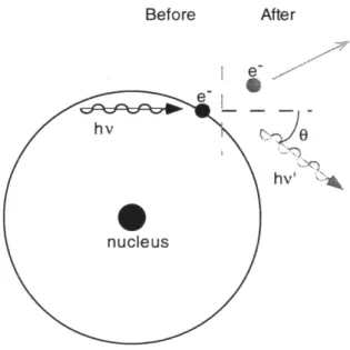
Another mode of interaction between photons and matter is Compton scattering. As described in Figure 2.1, an incoming photon interacts with an atomic electron and causes it to be ejected.

Before After

Figure 2.1. Schematic of the Compton scattering process

In contrast to photoelectric absorption, the incoming photon is not completely absorbed. Instead it scatters at an angle

e

I hv

hv

=

-1+- - 2(1-cose)

mec

Eq.2.2

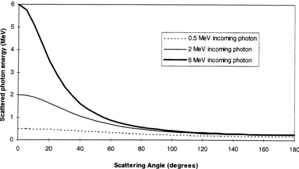
where me is the rest mass of the electron, such that mec2is equal to 511 keV. The binding energy Be of the electron is not taken into account in this formulation. The scattered photon energy as a function of () is shown in Figure 2.2.

5. 4 33 0 0 M 2 CD, 0 0 20 40 60 80 100 120 140 160 180

Scattering Angle (degrees)

Figure 2.2. Energy of Compton scattered photons as function of the scatter angle

One can distinguish a number of interesting features in these curves. First, when the angle of scatter 0 is close to 00, one finds, as expected by intuition, that the photon energy

is unchanged. At 900, the scattered energies for photons above 1 MeV converge towards

the rest mass of the electron, 0.511 MeV. Finally, at the backscattering angle 1800, the

scattered photon energies converge towards meC2/2.

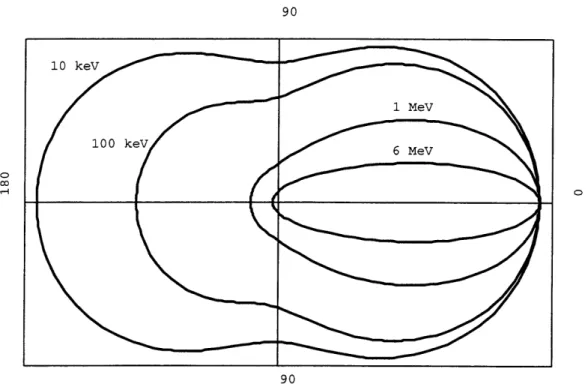
The angular distribution of Compton scattered photons is both a function of the angle 0 of this scatter with respect to the trajectory of the incoming photon, and of this photon's energy. The theoretical expression for this distribution is known as the Klein-Nishina formula [6]:

d

,

/

1

I+cos20)

2

d2 1 + a(1 - coso) 2

S2

A graph of this expression is shown in Figure 2.3, where it is evaluated for energies of 10 keV, 100 keV, 1 MeV and 6 MeV.

90

O

Figure 2.3. Polar plots of the probability of Compton scattering as a function of the scattering angle 0 for a

variety of photon energies .

In the context of computed tomography, it is important to note that the more energetic the photons, the shallower the angle of scatter will tend to be; and as a consequence, the photons scattered at small angles retain most of their energy.

2.1.3. Pair Production

Above a certain threshold, a photon's energy can be directly converted into matter. In this process, a particle and its corresponding antimatter conjugate are created. For reasons of conservation of energy, the pair production of an electron and its antimatter counterpart, the positron, requires a minimum photon energy equal to twice the electron rest mass me, i.e. 1.022 MeV. A schematic of this process is shown in Figure 2.4.

Before j! /1

,/1/

•

\\

\~

Figure 2.4. Schematic of the pair production process

As shown above, the pair production process requires the presence of a nucleus to satisfy the laws of conservation of energy and momentum. The electron and the positron have an equal kinetic energyTe,given by Eq. 2.4.

hv 2

T=--mc_{e 2 e} Eq.2.4

Because they are electrically charged, the electron and the positron rapidly loose their kinetic energy and nearly stop. Whereas the electron is absorbed by the medium, the positron interacts with an atomic electron and annihilates with it. As a result, two x-ray photons of 0.511 MeV each are created. Because the electron and positron involved are nearly at rest, the annihilation x-rays travel in nearly opposite directions.

Overall, the important features of the pair production process are its threshold of 1.022 MeV, and the creation of two lower energy x-rays emitted isotropically.

2.2. Photon Attenuation

The probability of interaction of a photon as it travels in a medium is constant. In

the case of a thin target of thickness L1x, the probability of interaction is proportional to this thickness Llx, with a constant of proportionality defined as p, the linear attenuation

coefficient. Given a number of photons No entering the thin target, the number that will

interact AN is given by Eq. 2.5.

AN = pNo -Ax Eq. 2.5

This model can be extended to thick targets by integrating Eq. 2.5 over a distance 1:

N(x) = NO - f N(x)dx Eq. 2.6

0

The result of this integral equation is given next:

N(x) = Noe -" Eq. 2.7

This equation shows that the number of photons in a target decreases exponentially. This model assumes that the photons that interact are removed completely, which is the case for the photoelectric effect, but is not in the case of Compton scattering nor pair production. Although we will adopt this standard attenuation model in the remainder of this text, the issue of scattered photons will be addressed in section 5.3.

The attenuation coefficient #u takes into account all three interaction types

described in section 2.1. It can be decomposed into three components, Lpe, ycs_, and Jpp,

representing the attenuation coefficient for the photoelectric effect, Compton scattering and pair production respectively. Because these phenomena rely on different physical basis, their importance is a function of the photon energy, the material density, and its composition.

The photoelectric effect attenuation coefficient per atom increases with the atomic number Z of the target material and decreases with the photon energy E. An approximate relation is given in Eq. 2.8 [6].

Zn

#pe C< E3.5"

Eq.

where n depends on the material and varies between 4 and 5. This equation signifies that the photoelectric effect is much more important for high Z materials such as tungsten (Z=74) and lead (Z=82) than for lower Z materials such as aluminum (Z=27). Also, one can expect that the photoelectric effect will be dominant at low photon energies, and will drop off quickly as the photon energy increases.

The attenuation coefficient for the Compton scattering process is almost independent of the atomic number Z, and generally decreases as the photon energy E

increases.

Pair production doesn't contribute to attenuation at all until the threshold energy 1.022 MeV is reached. Above this energy, the attenuation coefficient increases swiftly.

In terms of the atomic number, the coefficient per atom varies approximately as Z2_.

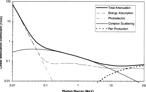
Figure 2.5 shows these coefficients for aluminum. [The coefficients where

calculated using the PhotCoef software package for IBM PC compatible, published by Applied Inventions Corporation].

E

00

Photon Energy (MeV)

Figure 2.5. Linear attenuation coefficients for aluminum for photon energies ranging from 10 keV to 100 MeV.

At energies below 100 keV, the photoelectric effect dominates all other phenomena due to its strong inverse dependence on E. As we increase photon energies, the probability of photoelectric absorption drops, and because the threshold for pair production hasn't been reached, the Compton scattering phenomenon dominates,

decreasing slowly with energy. Finally, for energies greater than 1.022 MeV, 1pp

increases slowly until it supersedes -cs between 10 and 100 MeV.

An interesting feature of Figure 2.5 is the energy absorption coefficient hA. As we

have seen, the amount of energy deposited by a photon depends on the interaction type. For the photoelectric effect, all the photon energy is deposited. This is apparent in Figure

2.5 at low energies when only ype is important and ILA=lpe. In Compton scattering, only a

fraction of the incoming photon energy is carried by the recoiling electron, meaning that

in the energy range in which #cs is dominant, the energy absorption coefficient YA is

production dominates, the energy carried by the annihilation x-rays is not accounted for in

MA, again meaning that yA<qu.

For a given target material and photon energy, the attenuation coefficient Y will be proportional to the target atom density, which in turn is proportional to the mass density p of the material in question. Because of this, it is often easier to use the mass attenuation

coefficient, nm. The definition of #m is given in Eq. 2.9.

M

Mm Eq. 2.9

We can now compare the attenuation properties of different materials. The following

figure shows the mass attenuation coefficient mm for air, water, aluminum and lead, for

photon energies ranging from 10 keV to 100 MeV.

1000

0.01

0.1 1 10

Photon Energy (MeV)

Figure 2.6. Mass attenuation coefficients of air, water, aluminum and lead as a function of photon energy

As we will see in section 2.4, an important feature of this graph is the fact that between 1 and 5 MeV the mass attenuation coefficient is independent of the material type, meaning that the attenuation coefficient y is proportional only to the material density p.

Before applying these observations to the experiment described in this text, we will examine how computed tomography relies on the concepts developed above.

2.3. Principles of Computed Tomography

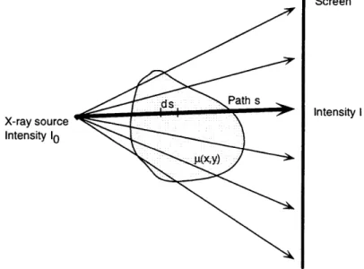
In standard radiography, x-rays are transmitted through an object, and the attenuation of these x-rays is measured using a film. A radiograph is essentially a map of this attenuation. Because the object under study is made of a variety of materials of varying densities, the attenuation coefficient y is a function of the position within the object. Measuring the attenuation of an x-ray beam along a given path allows one to calculate an average attenuation coefficient J . This concept is illustrated by Figure 2.7.

X-ray source Intensity 10

Screen

Intensity I

Figure 2.7. Schematic of a radiography experiment

The photon intensity I measured by the screen is related to the intensity Io emanating from the x-ray source by the following equation:

I = Ioe o" Eq. 2.10

The average attenuation coefficient along the path s is given by:

f (s')ds'

0=

In

Eq. 2.11

s I

The limitation of traditional radiography is apparent in this equation: the depth information in yu(s) is lost. Computed tomography allows one to obtain this information using a set of radiographs taken at a number of angles around the object. This process amounts to performing a Radon transform, which will now be described.

2.3.1. The Radon Transform

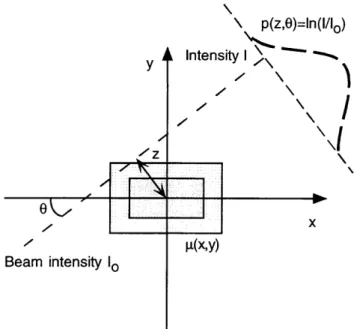
The linear attenuation coefficient y(x,y) within an object varies with position as shown in Figure 2.8.

n intensity _Io \ p(z,e)=In(I/1₀o) L Intensity I I /I

\

-J

Figure 2.8. Radon transform geometry

An x-ray beam traverses the object at an angle 0 from the x-axis, at a distance z from the center of the reference frame. The quantity p(z, 6) is a function of both z and 0. Its analytical form is:

p(z, ) =

f

This transformation from {x,y} to {z,O} is named the Radon transform [7]. The result of this transformation is a two-dimensional function called a sinogram. An example of an object and its corresponding sinogram are shown in Figure 2.9.

Bean

313 200 y o o x 200 e

o

o

Figure 2.9. Sample bitmap (left) and its corresponding sinogram (right)

When an x-ray CT experiment is carried out and a sinogram is obtained, the goal is to reconstruct the object map from the sinogram. The issue is therefore to process the sinogramp(

z,

2.3.2.

The Inverse Radon Transform

The Fourier transformF(w)of afunctionf(x) is defined as follows:

00

F(w)

=

f

The inverse Fourier transform is itself defined such that:

28

f (x) =

-

The Fourier transform of p(z, 0) along the z-axis is derived next:

P(wz ,6) =

J

= ff Iy(x, y)e-iw'(xcoso+ysinO)dxdy Eq. 2.15

= M(wx,wy,)

This result constitutes the central slice theorem. It states that the one-dimensional Fourier transform of the sinogram is equal to the two dimensional Fourier transform of the map of the object. The function yu(x,y) can now be obtained by taking the two

dimensional inverse Fourier transform of M(wx,wy).

u(x,y) = 2 M(wx ,w, )eiwx+wy)dwxdw,.

2r-Eq. 2.16

-42 f fP(wz,O)ei'wzlJldwzdO

0--where IJI is the Jacobian of the transformation from {wx,wy} to {wz 6], and equal to Iwzl.

If we denote the Fourier transform operation and its inverse as F and F1 _{respectively, the}

inverse Radon transform operation can be summarized as follows:

Yu(x,y) =

jF- iP(w,e).-we}dO

This function y at a point (x,y) is therefore proportional to the sum of the function inside the integral, evaluated along all paths traversing (x,y) and over a 1800 angular range. This

type of operation is called a backprojection. Equation 2.17 signifies that the linear attenuation coefficient distribution in an object can be reconstructed in five operations:

• obtain the sinogramp(z,O) experimentally,

• take the z-axis Fourier transform of p(z, 0) to obtainP(Wz,0),

• multiplyP(Wz,0) by the filter function Iwzl,

• take the inverse Fourier transformp'(z,0) of the result, • backproject this filtered sinogram.

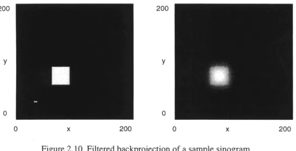
This algorithm for the reconstruction of J1(x,y) is known as the filtered backprojection (FBP) algorithm. The result of the FBP algorithm for the example of Figure 2.9 is now contrasted to the result of standard backprojection, for which no filter is applied to the sinogram. 200 y o 200 y o

o

o

Figure 2.10. Filtered backprojection of a sample sinogram (left) and unfiltered backprojection of the same sinogram

(right)

It is apparent that the IWzl filter described serves to compensate for the blurring effect apparent in the usage of unfiltered backprojection. This filter is appropriate if the region examined is sampled without noise and if the information one seeks to recover is bandwidth limited to less than half of the spatial sampling resolution. This is a result of the Nyquist sampling theorem [8], which states that· in order to properly reconstruct a

continuous signal limited in bandwidth to a frequency signal, it must be sampled at a

frequency equal to or greater than twice Qignt.

Nyquist theorem: amplin 2 2 .signal Eq. 2.18

Other filters exist that should be used when these conditions are not met [7]. This is in general the case.

Now that the mathematical foundation of x-ray computed tomography has been presented, we will explore the issue of the optimal photon energy for our experiment.

2.4. Photon Energy Requirements

The goal of this experiment is to obtain a two-dimensional map of the density changes within an sample of liquid and solid aluminum. As we have seen, x-ray CT will yield a map of the linear attenuation coefficient of the object under examination. Because the mass attenuation coefficients gm of liquid and solid aluminum are the same, dividing

p(x,y) by #m, Al will result in p(x,y), the quantity we are interested in.

A number of issues arise when one considers the fact that most x-ray sources are

not monoenergetic and that the object imaged is not exclusively composed of aluminum. These conditions imply that the map of p obtained by CT reconstruction will represent an average over all the energies present in the x-ray beam, as well as an average of the mass attenuation coefficients of the materials in the object under study. This is illustrated by the following equation.

Em (s)

p(z,6) = f dsp(s) jf (E',s).Lm(Z(s),E'IkE' Eq. 2.19

dN

wheref(E,s)= d is the energy distribution of the x-ray beam at the position s along the

dES

beam path. Indeed as an x-ray beam penetrates into a target, its spectrum changes due to the dependence in the interaction probability of a photon on its energy. Because lower energy photons have a higher attenuation coefficient, the lower end of the spectrum will tend to decrease in size with depth. This phenomenon is called beam hardening.

To reconcile Eq. 2.19 with Eq. 2.10, a solution is to choose the beam energy range so that #m remains independent of energy and material composition. Examining Figure 2.6 reveals that in the 1 to 3 MeV energy range these conditions are nearly satisfied. In this region, the mass attenuation coefficients of the variety of materials presented converge near 0.03-0.05 cm2/g. In addition, the coefficients vary slowly with energy.

Assuming a mass attenuation coefficient of 0.04 cm2_{/g for a photon energy in the}

range described above and considering an aluminum sample of density 2.7 g/cm3_{, we}

calculate an attenuation coefficient of 0.11 cm'- _{. To better understand this number, it is}

preferable to introduce the concept of the half-value layer (HVL). The HVL is defined as the thickness of target material that will diminish the intensity of a photon beam by a half. The relationship between the HVL and the attenuation coefficient y is simple:

ln 2

HVL - JEq. 2.20

The half-value layer of aluminum for the case considered above is calculated to be equal to 6.4 cm. As we will see, this number is appropriate for a CT application in which the studied object is on the order of a few tens of centimeters in size, such as in this experiment.

These observations lead one to consider an x-ray source that will produce a beam the energy spectrum of which shows strong component between 1 and 3 MeV. The MINAC 6 linear accelerator is a source that meets these criteria, and is the topic of the next chapter.

3.

X-RAY SOURCE: THE LINAC

As we have seen in Chapter 3, high-energy photons are an appropriate particle to use as a probe to measure the density fluctuations within an aluminum sample such as the one used in this experiment. There are several sources of such high energy photons, two of which are of particular interest. The first one is a radioactive source that emits gamma rays. The important characteristics of radioactive emitters are the following:

* the photons emitted are monoenergetic,

* the rate of emission follows an exponential decay which can be characterized by a half-life,

* the source cannot be turned off.

An example of such a source would be Cobalt-60 (Co60), which emits two

gamma-rays per disintegration, with energies of 1.17 and 1.33 MeV. The half-life of Co60

is 5.3 years, removing the concern with the exponential decrease in the source activity during an experiment that can arise with shorter half-lives. On the other hand, a long half-life translates into a smaller specific activity, which is equal to the activity per unit mass of the sample. The highest specific activities achievable today for Co60 are on the

order of 200 Ci/g [9], where one Curie corresponds to 3.7x10'0 _{disintegrations per}

second. As we will see further, these characteristics do not compare favorably with our second source of high energy photons, the linear accelerator.

3.1. Principles of the Linac

Traditionally, intense x-ray beams are produced using x-ray tubes. The photons are emitted when bombarding a target with high energy electrons. The electrons are produced by heating a thin filament surrounded by a cup-shaped cathode. As the electrons boil off the filament, they find themselves accelerated in a DC electric field towards an anode. The anode serves as the target for the bombardment, and is at an electric potential that is up to several hundred kilovolts greater than that of the cathode.

After acceleration, the electrons are nearly monoenergetic and carry an energy in electron-volts that is equal to the voltage applied between the cathode and anode. As the electrons impinge upon the target, they are slowed down through collisions with the electrons surrounding the atoms in the material, and are submitted to abrupt accelerations. As electromagnetic theory states, accelerating charged particles emit radiation. In the case of charged particles colliding with a target, the photons produced are called bremsstrahlung radiation. One property of this type of radiation is that it consists of photons that carry a spectrum of energies, the maximum of which is equal to the energy the electrons are accelerated to.

One drawback of traditional x-ray tubes is that the energy of the accelerated electrons is limited to a few hundred kilovolts because of the risks of arcing between the anode and the cathode. To reach higher energies, machines were developed that did not rely on DC electric fields for acceleration, but rather on radio-frequency (RF) alternating electromagnetic fields. These machines are linear accelerators (linac), and we will now describe the principles behind their operation, as well as the characteristics of bremsstrahlung radiation.

3.1.1. Electron Acceleration in Linacs

The contrast between linacs and x-ray tubes lies in the manner in which the

electrons are accelerated. Linear accelerators are classified into two categories:

traveling-wave accelerators, and standing-wave accelerators. Both are based upon a

waveguide structure divided into sections separated by conducting discs. Pulses of electromagnetic radio-frequency fields are fed into this structure. In a traveling-wave accelerator, the wave travels only in one direction. In a standing-wave machine, two waves of equal amplitude travel in opposite directions, creating a standing pattern similar to that observed in vibrating strings. We will now discuss how the electric field patterns

in both systems work to accelerate a fraction of the electrons to very high energies.

Electromagnetic fields travel at the speed of light c, equal to 3x10'o m/s. As a consequence, the wavelength A is inversely proportional to the frequency v of the wave following the relation:

C

Eq. 3.1

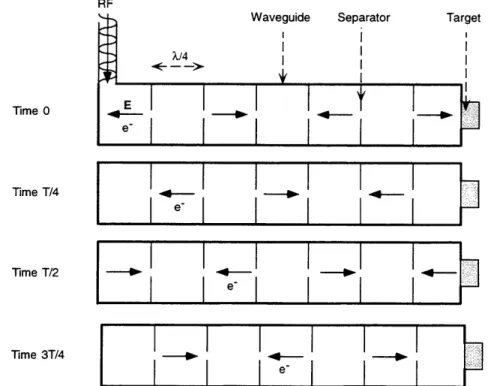
Let's consider a waveguide structure in which each section is separated by a quarter of a wavelength, X/4. In the case of a traveling wave linac, we describe the evolution of the longitudinal component of the electric field in Figure 3.1.

RF Time 0 Time T/4 Time T/2

e"

e-I- -

l

I

I

Figure 3.1. Time evolution of the longitudinal electric field in a traveling wave linac

In this illustration, time is expressed in terms of the period T equal to the inverse of the frequency, 1/v. The arrows inside the waveguide indicate the direction in which the electric field points. In a quarter of a period, the wave propagates by a distance equal

to ?/4. If electrons, represented by the symbol e-, are injected into the waveguide at a

velocity close to that of light, they will be accelerated over the entire length of the linac by the longitudinal component of the electric field E . The acceleration scheme is slightly

different in a standing wave linac, as illustrated in Figure 3.2.

I E

Time 0 Time T/4 Time T/2

I I I

I

I

o

lI

I

I

I I°

I I I

e

-

i

Time 3T/4

Figure 3.2. Time evolution of the longitudinal electric field in a standing wave linac

In the standing wave linac, two RF waves travel in opposite directions and either cancel or re-enforce each other. In contrast with the traveling wave accelerator, the electrons are accelerated half of the time. This loss is made up by the electric field which is twice as strong. The overall acceleration is equal in both standing wave and traveling wave linacs.

In the previous treatment, we assumed the electrons entered the accelerating structure at a velocity close to c. The velocity of a particle v is related to its kinetic energy

T by the following relativistic formula:

-11

Eq. 3.2

T = m_o

where mo is the rest mass of the particle. If the kinetic energy of an electron is equal to its rest mass mo=0.511 MeV, one finds that P=v/c is equal to 0.87, meaning that the electron travels at 87% of the speed of light. At energies of 1 MeV and above, our assumption that the velocity of the electron is constant is justified. At lower energies, the acceleration is achieved by making the initial waveguide cells shorter in length, so that the velocity of the electrons matches the phase velocity of the electromagnetic wave. In this way, the electrons that find themselves in phase with the accelerating portion of the longitudinal electric field receive energy from the RF field and can be accelerated in short distances.

The development of linacs was in great part possible because of the emergence of devices capable of creating strong pulses of RF radiation in the decimeter range and

below. Such devices, magnetrons and klystrons, were invented to satisfy the

requirements of radar during World War II [10] [11 ].

3.1.2. Bremsstrahlung Radiation

X-rays are produced by smashing the high energy electrons produced by either an x-ray tube or a linac into a target. Electrons lose their kinetic energy through two types of interactions. First, as they collide with the electronic cloud surrounding an nucleus, they can excite or ionize an atom. This results in the heating of the target and in the production of characteristic x-rays that are radiated as an electron drops into a lower energy level after excitation or ionization.

The second process occurs as an electron travels in the vicinity of a nucleus. Its trajectory bends significantly due to the electric attraction between the negative charge of

the electron and the generally greater positive charge of the nucleus. The nucleus

essentially remains in place during this interaction due to its rest mass which is three to five orders of magnitude greater than that of the electron. According to electromagnetic theory, as a charge accelerates, it emits radiation. An electron slowing down in the presence of a nucleus consequently emits bremsstrahlung ("braking radiation" in German) radiation. Depending on how much kinetic energy the electron loses, the radiation can consists of a photon carrying up to the full electron energy. In the thin target approximation, in which the target is considered thin enough that each electron will

at most collide once, the intensity of the emitted radiation is constant from zero to E, the electron kinetic energy [9]. One can extrapolate this result to a thick target by realizing that after each collision, an electron will emit bremsstrahlung radiation similar to that described above for the thin target, but with a maximum energy reduced to the electron energy after the first collision. By superposing all these individual thin target spectra, one obtains a thick target spectrum similar to the one shown in Figure 3.3.

Photon A

Intensity - - - - Thin target spectrum

-- Thick target spectrum

- - 1 - -- - Filtered thick target spectrum

Electron kinetic energy

----

.. .r_

Figure 3.3. Thin and thick target bremsstrahlung spectra for

an electron kinetic energy E.

Of course when photons travel through a thick target, they are attenuated via absorption and scatter. As seen in Section 3.2, low energy photons are absorbed more efficiently than higher energy radiation. As bremsstrahlung photons travel through the thick target, the low energy part of the spectrum is preferentially absorbed by the medium, resulting in a drop in intensity in the lower part of the spectrum. This is illustrated by the filtered thick target spectrum curve in Figure 3.3.

It is of interest to note that the ratio of the radiative (bremsstrahlung) to the collisional stopping power is given approximately equal by the following equation:

(-dE/dx)

r,

ZE

(-dE/dx) coI =800

Eq. 3.3

Here dE/dx is equal to the energy loss rate of the electron over a distance dx along its travel path, Z is the atomic number of the target material, and E is the electron kinetic energy, expressed in MeV. This equation will prove useful in justifying the choice of tungsten as the target material for the production of x-rays in MINAC 6, which will be done in section 3.2.3.

3.2. Characteristics of MINAC 6

The MINAC 6 linear accelerator is manufactured by Schonberg Research Corporation, of Santa Clara, CA. We will examine its physical characteristics, its operating characteristics, and the type of x-ray beam it creates.

3.2.1.

Physical Characteristics

The MINAC 6 accelerator consists of six components. Their name, dimensions and weight are described in Table 3.1.

Component name Modulator

RF Unit X-Ray Head Water cooling system

Control Console Remote Monitor and Interlock

Dimensions (I x w x h) [cm] 89 x 51 x 58 102 x 46 x 46 69 x 10 x 18 66 x 53 x 97 64 x 51 x 28 36 x 38 x 33

Table 3.1. Components of the MINAC 6 linear accelerator.

Weight 181 kg 113 kg 41 kg 145 kg 18 kg 11 kg

The various modules are interconnected as shown in Figure 3.4.

Control Console Remote Interlock and Alarm Unit

Power Modulator Unit

I I I I I I-I X-rays

Figure 3.4. Diagram of the MINAC 6 components

3.2.2.

Operating Characteristics

The modulator contains circuits that produce high voltage pulses used by the magnetron and the x-ray head. This assembly can produce pulses between rates of 50 and 200 pulses per second. Each pulse lasts 4 gs, with a rise and fall time of 0.5 gs

The RF unit contains the magnetron which produces pulses of radio-frequency radiation. It is driven by the high voltage pulses of the modulator. The radiation is produced in the X-band frequency, at exactly 9303 MHz. It is output via a flexible

The x-ray head is responsible for accelerating electrons and producing bremsstrahlung x-rays. It includes an electron gun driven by the modulator's voltage pulses, a 52 cm long standing-wave accelerating section, a high-density tungsten target, and a collimator. The x-ray head receives the RF waves from the flexible waveguide via a side port. The electron current during a pulse is 50 rnA, with an average current of 50 JlA, corresponding to a 1000-to-l duty factor. The electron gun is a triode-type gun, and injects 15 keV electrons into the accelerating section. Before colliding with the target, the electrons reach an energy of 6 MeV. The target itself is made of a thin sheet of tungsten. The x-rays produced are then restricted into a 30° cone by a tungsten collimator.

The MINAC 6 x-ray head is shown in Figure 3.5, where the collimator is visible as a metallic cylinder on the right. The center section, in white, is the housing for the RF coupling window and the connections for the water cooling tubes. On the left, one can distinguish the high voltage pulse plug.

Figure 3.5. Photograph of the MINAC 6 x-ray head

The heat exchanger is a closed-loop water-cooling system that circulates water at 20°C through the RF module and the x-ray head to dissipate the heat produced by those units.

The control console is used to operate the linac and monitor its performance. It is equipped with readouts for the radiation output and the status of the accelerator. It also features a series of LED's that turn on in a sequence corresponding to the power-on procedure.

Finally, the remote interlock and alarm unit is designed to reside in the vault in which x-ray head is used. Prior to the emission of any radiation, a visual and audible alarm is given, warning any personnel that the beam is about to be turned on. A "panic button" is located on the unit, allowing anyone in the facility to power down the system and avoid exposure to harmful radiation in the case of an operational error.

3.2.3. X-Ray Beam Characteristics

The atomic number of tungsten is 74, and its density is 17.3 g/cm3_{. Applying Eq.}

3.3, one finds that for 6 MeV electrons 36% of the lost electron kinetic energy is used for the creation of bremsstrahlung x-rays. The high atomic number of tungsten is indeed a major reason for its choice as a target for the production of x-rays in most devices. Its high density contributes to keeping the electron paths short; this translates into a smaller spot size than obtainable with other materials. The MINAC 6 target consists of a 0.889 mm thick tungsten sheet welded to a .965 mm thick copper support. In addition a 1 mm thick lead sheet is added at the exit of the collimator. The collimator itself is made of tungsten because its high density translates into a large linear attenuation coefficient. The role of the collimator is to restrict the x-rays emitted by the target into a 300 cone. It is configured as a 9.5 cm long cylinder with a cone-shaped hole the aperture of which is 4.45 cm.

Using the geometry specified above as an input to a photon transport simulation program, one can compute the energy spectrum of the MINAC 6 x-ray beam. This was done using MCNP (Monte Carlo N-Particle Transport Code System) published by the Los Alamos National Laboratory, New Mexico. A total of 400,000 electrons were simulated. The x-ray energy flux was measured at a distance of 1 m away from the tungsten target, and integrated over an angle of 300. Energy bins 50 keV wide where used to tally the

measured photons. The MCNP input code is given in Appendix A. The spectrum obtained is shown in Figure 3.6.

0.3 0.25 0.2 0.15 0.1 0.05 0 1 2 3 4 5 6 Energy (MeV)

Figure 3.6. Calculated MINAC 6 photon number spectrum dN/dE

This spectrum can be more easily compared with the type of result expected from section

3.1.2 if it is expressed in terms of intensity rather than photon number. This

transformation is carried out by multiplying dN/dE by E. The resulting intensity spectrum is presented in Figure 3.7.

0.12 0.1 -0.08 S0.06- 0.040.02 -0 0 1 2 3 4 5 6 Energy (MeV)

Figure 3.7. Calculated MINAC 6 photon intensity spectrum dU/dE

As expected from theory, the photon intensity decreases linearly with energy. The drop in the low end of the spectrum is caused by the shielding effect of the lead sheet. Indeed, because the low energy photons are subjected to a greater linear attenuation coefficient, they are more easily stopped by the thin sheet. This is a manifestation of the beam hardening phenomenon discussed in section 2.4. As expected, no photons are observed above 6 MeV, the electron energy.

This spectrum can be used to calculate the average energy of the photons. The result was found to be 1.29 MeV. This number may appear low, but one must remember that as the beam progresses through the imaged object, the low end of the spectrum will be filtered out, leading to an increase of the average energy. Overall, the average energy of the beam will remain within the target range specified in section 2.4.

The MINAC 6 linac produces 300 R/min of ionizing x-rays. One Roentgen [R] is

equivalent to a charge of 2.58x10 4 _{C created in a mass of one kilogram of air by ionizing}

photons. The average energy required to ionize an atom in air is equal to 34 eV. Because

each ionization involves the creation of a charge of 1.6x10-1 9 C, the MINAC 6 output can

COI 0

_{00 00 00 0}

00

*004

0

therefore be translated into an energy deposition rate of 2.7x10'7 _{eV/kg/s, or 2.7x10}8 MeV/g/s.

If we assume that this energy is deposited in a volume of area A and very small thickness Ax, we can calculate the photon flux 0 traversing the volume using the following equation:

AEdeposited =. A. E.-

(A.

1 AE 1 AE

E gm,air (A -AX -Pair) -E E ff,,air

Eq. 3.4

where E is the average energy of the photons in the beam, ffm,air is the average mass

attenuation coefficient of air for energy deposition in the beam, and AM is the mass of the volume of air we consider. As established from the beam spectrum analysis, the average

energy of the photons is E =1.29 MeV. To determine ,air,,' we consider the following

figure. 1000 100 10 0.01 0.01 0.1 1 10

Photon Energy (MeV)

Figure 3.8. Energy absorption mass attenuation coefficient of a variety of materials for energies ranging from 10 keV

At an energy of 1.29 MeV, the mass attenuation coefficient of air for energy absorption is

0.025 cm2/g. Using this value in Eq. 3.4, we obtain a photon flux equal to 0 = 8.4 x 109

photons/cm2/s.

This photon flux figure can be used to verify the validity of the Monte Carlo simulation used to obtain the spectrum. Its results indicate that the photon flux per

electron at 1 meter is equal to 3.25 x 10-5 _{photons/electron/cm}2_{. Dividing the 50 gA}

electron output of MINAC 6 by the charge of the electron e, equal to 1.6 x 10-19 _{C, tells}

us that MINAC 6 produces 3.13 x 10 14 electrons/s. Multiplying this number by the

predicted photon flux per electron gives us the photon flux per unit time. The result,

OMCNP = 1.02 X 10lo photons/cm2/s, is close to the figure obtained in the previous

paragraph from the MINAC 6 specifications. This is a good indication that the Monte Carlo simulation's results are valid.

The determination of the x-ray properties of the MINAC 6 beam are essential to the characterization this experiment's performance. Before that step can be carried out, it is necessary to specify the properties of the aluminum sample we propose to image as well as those of the apparatus needed to create the stable solid/liquid phase transition. This is the topic of the next chapter.

4. SOLIDIFICATION FRONT

In computed tomography, the object imaged needs to be scanned through an angular range of at least 1800. For this reason, we need to have a system that will rotate an aluminum sample. Before we describe this system, the experimental setup of the sample is presented.

4.1. Furnace and Cooling System

A cylindrical furnace is used to create an aluminum sample in which a stable

solid/liquid phase interface can be maintained. A schematic of the cross section of this furnace is shown in Figure 4.1.

1.2 mm thick steel .40 cm. Hea Air Cr 10.50 cm. cm. 7.60 cm. Figure 4.1. Cross sectional schematic of furnace with

This furnace is integrated into the experimental setup shown in Figure 4.2. This schematic shows a cylindrical furnace 16 inches high manufactured by Mellen, Webster, NH. At the core of the furnace is a cavity in which lies a graphite crucible. The crucible is heated by resistive heating elements placed around the perimeter of the cavity. These heating elements are in turn surrounded by low density insulation material. Finally the furnace is surrounded by a thin steel sheet to provide protection to the insulation. The following figure shows a cross sectional view of the furnace.

Insu

Crn

Heater Eler

Figure 4.2. Schematic of the experimental setup for the creation of a liquid/solid interface in aluminum

The temperature of the air gap is measured by a built-in thermocouple. The furnace controller monitors this temperature and pulses current through the heating elements to regulate this temperature.

The cavity in the crucible is topped by an insulated cover. A cooling tube penetrates through the cover into the inside of the crucible. As compressed air flows down the inner core (OD of 1.59 cm) of the cooling tube and up the outer boundary (OD

An interesting feature of this experimental setup is its cylindrical symmetry. Because of it, the solidification front is also expected to show some radial symmetry, which should allow an improved analysis of the solidification front geometry.

4.2. Motion system

To allow the furnace to be rotated through any angular range, it is placed on a rotational table driven by stepping motor. The rotational stage itself is placed on top of a translational stage, which allows the furnace's position within the x-ray beam to be changed. The tables are manufactured by New England Affiliated Technologies, Lowell, MA. The stepping motors are controlled by an amplifier manufactured by Nulogic, Needham, MA.

5.

DETECTOR SYSTEM

X-rays are an appropriate probe for computed tomography because they are a

highly penetrating radiation. This very property makes them difficult to detect. As we

will see, ray detection relies on sensitive measurements of the charge created by an

x-ray photon as atoms become ionized. There are several methods to perform this

measurement which we will explore in the following section. As will appear from this

review, the combination of cadmium tungstate (CdWO4) scintillation crystals and

photodiodes is an appropriate choice for our application. Our experimental detection setup will be described, with particular attention focused on the issue of Compton scattered photons and means to reduce their contribution.

5.1. Principles of X-Ray Detection

The photoelectric effect, Compton scattering and pair production all lead in the

end to ionization of atoms in the target material. The task is to find methods of

measuring the extent of this ionization, and to detect it fast and efficiently. We will review the most widely used techniques used to achieve this, and will determine which characteristics are sought in an x-ray CT context.

5.1.1. Gas-filled Chambers

A very popular means of x-ray detection relies on a gas-filled chamber in which a

strong electric field is generated. The basic principle behind the operation of such

devices is the following. As radiation penetrates the volume inside the chamber, gas atoms and molecules ionize into separate electrons and heavy ions. An anode and a cathode connected to a voltage source cause a strong electric field to pervade within the volume, and because of their opposite charges, the electrons and ions diffuse towards the