Demand simulation for dynamic traffic assignment

(1)

Demand Simulation for Dynamic Traffic Assignment

Constantinos Antoniou

Diploma in Civil Engineering

National Technical University of Athens, Greece (1995) Submitted to the Department of Civil and Environmental

Engineer-ing in partial fulfillment of the requirements for the degree of Master of Science

at the

MASSACHUSETTS INSTITUTE OF TECHNOLOGY January 1997 .

©

A uthor ... ... ---Civil and Environmental Engineering Department

January 24, 1997

Certified by ... ...-- ... ... Moshe Ben-Akiva

Professor of ivi and Environmental Engineering Thesis Supervisor

Certified by ... ... ... .. Michel Bierlaire Research Associate, Center for Transportation Studies Thesis Supervisor

Certified by ...

Rabi Mishalani Research Associate, Center for Transportation Studies Thesis Supervisor

Accepted by ... ...

Joseph M. Sussman -rs; s . Chairman, Departmental Committee on Graduate Studies

OF :TECH1NOLCGY

JAN 2

9 1997

(2)

(3)

Demand Simulation for Dynamic Traffic Assignment

by

Constantinos Antoniou

Submitted to the Department of Civil and Environmental Engineering on January 24, 1997, in partial fulfillment of the requirements for the degree of

Master of Science

Abstract

In this thesis a pre-trip demand simulator with predictive capabilities and explicit simulation of the response of the travelers to real-time pre-trip information is proposed and implemented. The demand simulator is an extension of conventional OD estimation models aimed at overcoming their inability to explicitly capture the effect of information on demand. This is achieved by explicitly simulating driver behavior in response to both descriptive and prescriptive information at the disaggregate level.

The true demand can be constructed from the historical with the addition of two systematic deviations -the effect of information in the demand and the daily demand fluctuations- and a random error. Conventional OD estimation models do not take explicitly into account the first systematic deviation and, hence, their estimation accuracy may be limited. In the proposed demand simulator, the systematic component of the deviation that is due to the available information is captured by a set of disaggregate behavioral models which update the historical demand. The OD estimation uses the updated OD matrix, instead of the historical OD matrix itself, as a starting point to compute an estimated OD matrix consistent with the observed link counts.

A series of case studies are performed to illustrate some of the capabilities and assess some of the properties of the demand simulator, as well as investigate some of its potential shortcomings. Furthermore, a framework that can be used for a more comprehensive evaluation of the demand simulator is presented.

Thesis supervisor: Moshe Ben-Akiva

Title: Professor, Department of Civil and Environmental Engineering Thesis supervisor: Michel Bierlaire

Title: Research Associate, Center for Transportation Studies Thesis supervisor: Rabi Mishalani

(4)

Acknowledgments

I would like to thank my thesis supervisors Professor Moshe Ben-Akiva, Michel Bierlaire, and Rabi Mishalani for the guidance, advise and constructive feedback that they provided at all stages of this research.

I would also like to thank the staff of the MIT ITS Program, who provided a friendly research environment, and valuable information and help every time it was needed.

I am also thankful to Oak Ridge National Laboratory and Federal Highway Administration (FHWA) for financially supporting this research.

I would also like to thank my friends and fellow students that made MIT a unique experience and taught me a lot of things.

(5)

4.2.2 Computational Efficiency 61 4.2.3 Numerical Robustness 62 4.3 Requirements 62 4.3.1 Design Flexibility 63 4.3.2 Element Access 64 4.3.3 Memory Requirements 65 4.4 Objects 66 4.4.1 List of Objects 66 4.4.2 Object Associations 67 4.5 Implementation Issues 69 4.5.1 Off-line Disaggregation 69

4.5.2 Pre-Trip Behavioral Model 70

4.5.3 Aggregation 70

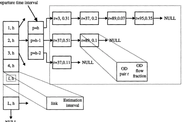
4.5.4 OD Estimation and Prediction Model 70

4.5.5 On-line Disaggregation 74 5. Evaluation 76 5.1 Scenarios 77 5.1.1 Network (A) 77 5.1.2 Historical demand (B) 79 5.1.3 Population-wide characteristics (C) 81 5.1.4 Pre-trip behavior (D) 82

5.1.5 En route behavior (E) 87

5.1.6 Guidance (F) 88

5.1.7 Habitual travel time data (G) 88

5.1.8 Link Counts (H) 88

5.1.9 Assignment matrices (I) 89

5.1.10 Transition matrices (J) 89

5.1.11 Error covariance matrices (K) 89 5.1.12 Initial state vector covariance (L) 90

5.2 Impact of Behavioral Update 90

5.2.1 Description of the process 90

5.2.2 Analysis of the Results 91

5.2.3 Conclusions 93

5.3 Stochasticity Analysis 93

5.3.1 Description of the Process 93

5.3.2 Analysis of the results 94

5.4 Sensitivity to Input 97

5.4.1 Description of the Process 97

5.4.2 Analysis of the results 99

(7)

6.1 Summary 105

6.2 Further Research 108

6.2.1 Extensions of Performed Tests 108

6.2.2 Assessment of Real-time performance 109

6.2.3 Evaluation of the Demand Simulator 110

(8)

List of Figures

Figure 1. Structure of the DynaMIT system 14

Figure 2. Representation of demand estimation 16

Figure 3. Pre-trip Demand Simulator 26

Figure 4. Simple road network with overlapping paths 35

Figure 5. Structure of the C-logit model 35

Figure 6. Habitual path choice generation 38

Figure 7. Pre-trip choice tree in the case of descriptive information 41 Figure 8. Pre-trip choice tree in the case of prescriptive information 46

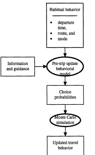
Figure 9. Travel behavior update process 48

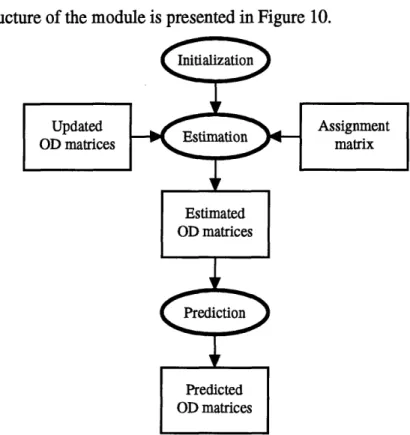
Figure 10. Estimation and prediction structure 55

Figure 11. Association example 60

Figure 12. Multiplicity example 60

Figure 13. Aggregation example 60

Figure 14. Inheritance example 61

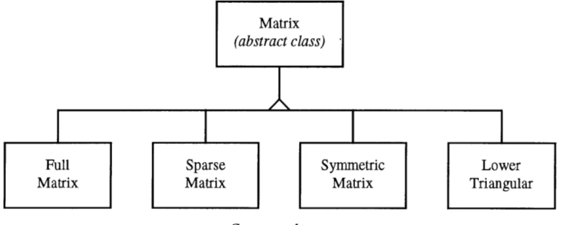
Figure 15. Matrix Classes 63

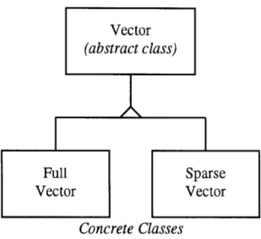
Figure 16. Vector Classes 64

Figure 17. Read-write iterator inheritance 65

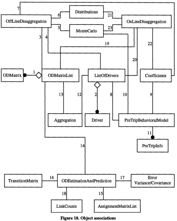
Figure 18. Object associations 68

Figure 19. ODMatrix data structure 73

Figure 20. Assignment matrix data structure 74

Figure 21. Map of the network 78

Figure 22. Schematic representation of the network 79

Figure 23. Demand pattern 80

Figure 24. Impact of behavioral update process overview 91

Figure 25. Deviation of updated from historical demand 92

Figure 26. Stochasticity analysis process overview 94

Figure 27. Total updated demand 95

Figure 28. Distribution of total updated demand values 96

Figure 29. Total updated demand standard deviation 96

Figure 30. Sensitivity process overview 98

Figure 31. Deviation of updated demand due to perturbation of the behavioral parameters 101 Figure 32. Deviation of estimated demand due to perturbation of the behavioral parameters 101 Figure 33. Relative error in the updated and estimated demand due to perturbations in the behavioral

parameters 102

Figure 34. Deviation in updated demand due to perturbation of the historical demand 102 Figure 35. Deviation of estimated demand due to perturbation of the historical demand 103 Figure 36. Relative error in the updated and estimated demand due to perturbations of

historical demand 103

Figure 37. Relative errors in estimated link flows due to perturbation in the historical OD flows 104

(9)

List of Tables

Table 1. List of variables for travel behavior models 29

Table 2. List of supercripts of coefficients for travel behavior models 31 Table 3. List of subscripts of coefficients for travel behavior models 32 Table 4. List of subscripts of structural coefficients for travel behavior models 32

Table 5. OD matrix for 3rd interval (7:30-7:45) 80

Table 6. Generated OD matrices 81

Table 7. Population-wide characteristics distribution 82

Table 8. Travel time profiles 84

Table 9. Estimated coefficients for the behavioral model 86

(10)

1. Introduction

Road traffic congestion and all the side-effects it has on the environment, productivity and mental state of the people, is one of the leading problems of cities today. Congestion steadily increases and the conventional approach of building more roads is faced with skepticism for a variety of political, economic, social, and environmental reasons. The realization that the existing terrestrial infrastructure can indeed perform better than it is doing at present, as a result of better utilization, led to the Intelligent Transportation Systems (ITS) initiative, which was introduced in the late 80s as Intelligent Vehicle Highway Systems (IVHS). For an overview of ITS, the reader is referred to Sussman (1992).

ITS is a broad term used to describe a variety of advanced technologies in the areas of advanced communication, computers, information display, road infrastructure, traffic control systems and advanced vehicle control systems. It envisages the

development of a Dynamic Traffic Management System that would, in real-time, attempt to improve capacity utilization by:

* Providing both pre-trip and en route information to motorists with respect to optimal paths to their destinations, and

* Using advanced traffic control systems that are adaptive to rapidly changing traffic conditions in real-time.

Congestion management measures can be categorized as either demand-based or supply-based. Supply-based measures are intended to increase the existing capacity of the system in order to improve the traffic flow for all modes. These measures include signal control improvements, incident management and preferential treatment of high occupancy vehicles (HOV) and public transit vehicles. Incident management refers to the necessary actions that need to be taken in real time to mitigate the effect of an incident on the network and alleviate the congestion that it may generate. The area of ITS that deals with these traffic management schemes is called Advanced Traffic Management Systems (ATMS).

Demand-based measures, on the other hand, are designed to reduce car demand on the system by increasing vehicle occupancy and public transit share, distributing the travel demand over time (peak spreading) and distributing the travel demand more uniformly on the traffic network. Demand-based systems rely heavily on the availability

(11)

of reliable, real-time information about the traffic conditions in the network. Collected information, such as current travel times and speeds on links, can be used as is or as the basis for the calculation of more complex information, such as the shortest path for a given origin-destination (OD) pair. These systems can improve the information available to the travelers by updating them about current and anticipated conditions on the roadway and transport network in general, and providing route guidance, using a variety of audio and visual means, both in-vehicle and on the roadway and other transport facilities. The disseminated information assists the individual travelers in decisions about their travel patterns.

A particular sort of demand-based measures take advantage of technological advancements, such as Advanced Traveler Information Systems (ATIS), for the faster and more effective dissemination of real-time information to travelers. Information can be provided either in the pre-trip stage or en route. Pre-trip information can be used by the travelers for departure time, route and mode choice. Furthermore, the travelers may decide to change their destination or cancel the trip altogether in response to pre-trip information. On the other hand, the effect of information available en route is usually restricted to subsequent route switching decisions. Nevertheless, it is theoretically possible to have mode choice made en route, e.g. in the case of a driver deciding to use a park-n-ride facility and switch to transit for the remainder of the trip, instead of driving.

A desirable feature of such ATMS and ATIS efforts is the ability to predict future traffic, since without projection of traffic conditions into the future, control or route guidance strategies are likely to be irrelevant and outdated by the time they take effect. In predicting traffic, however, it is essential that the effect of the provided information and guidance on travelers' travel decisions and, consequently, the network's traffic conditions is captured. Otherwise, the information and guidance will not be reliable.

In this thesis, a pre-trip demand simulator which captures the effect of information on estimating and predicting future roadway traffic demand is designed and implemented. The simulator uses disaggregate behavioral models to predict the drivers' travel behavior in response to real-time pre-trip information, and an aggregate OD estimation and prediction model.

1.1 Background

A congestion management tool that has been under investigation over the past years is Dynamic Traffic Assignment (DTA). A DTA system uses historical and real-time information to estimate and predict traffic and, consequently, provide travel information

(12)

and guidance. Real-time information about the traffic conditions on the network is essential in the performance of a DTA system, since this is the base of the generated guidance. In addition of being a necessary element of ATIS, DTA is also an essential element of ATMS. Travel guidance will be more effective when guidance information is provided as a component of an integrated approach including advanced traffic management and road pricing.

In this context, MIT Intelligent Transportation Systems (ITS) Program is developing DynaMIT (Dynamic Network Assignment for the Management of Information to Travelers), a DTA system that generates guidance based on predicted traffic conditions. Provided information can be either descriptive or predictive. Descriptive guidance provides tripmakers with information on network conditions so that they can make better decisions about departure time, mode and route choice. Prescriptive guidance consists of actual recommendations about route choice which users decide whether to

accept (comply) or reject. The way information is communicated may affect drivers' compliance rates. For example, based on driver simulation experiments, some researchers have reported higher compliance with prescriptive information when descriptive information is also presented (Bonsall, 1992, and Kitamura and Jovanis, 1991).

The assumptions made about user tripmaking behavior, and particularly about user response to travel choice guidance information, are central to any procedure which attempts to generate such information. Hence, different categories of user behavior are represented in the form of user classes in DynaMIT. In this context, a user class is a

particular combination of access to information (e.g. through an in-vehicle unit, a i roadway sign or a radio broadcast) and user behavior parameters (e.g. utility function

specification and coefficients) so that the reaction of different tripmakers to the provided information is taken into account (e.g. different degrees of compliance to guidance recommendations).

The structure of the DynaMIT system is shown in Figure 1. DynaMIT simulates both demand and supply. The demand is simulated by the demand simulator which estimates and predicts the demand in the network, taking into account the effect of available information. The supply (traffic) simulator then assigns this demand on the network and simulates the vehicles' trips considering en route demand modifications due to response to guidance. Using historical data and data from the surveillance system as input, an iterative process between the demand and the supply simulator is used to obtain a consistent estimate of the current state of the network in terms of OD flows, link flows, queues and densities. This is an important task, since information obtained from the

(13)

traffic sensors is generally sparse, i.e. the link counts are known only for a fraction of the links. Therefore, estimation is required to provide a complete picture of traffic conditions. The demand simulator incorporates an OD estimation model, which uses historical OD flows, real-time measurements of actual link flows on the network, and estimates of assignment fractions (the mapping of OD flows to counts) to estimate the true OD flows. The demand simulator is also sensitive to the information provided to the drivers. This information represents the true conditions on the network. By taking this into account, the simulator updates the historical demand in response to information from the network and uses this updated historical demand as a starting point for the estimation. Therefore, behavioral models which update the historical OD flows before they are used by the OD estimation model are incorporated in the demand simulator. As a result, the updated OD matrix already incorporates changes that took place in response to guidance and information.

The supply simulation model simulates the actual traffic conditions on the network. Inputs include OD flows estimated by the OD estimation model, network capacities and traffic dynamic parameters, as well as prior control strategies and guidance broadcast. The supply simulator outputs an estimate of the traffic conditions on the network, including link flows. These link flows will generally be different than the actual link counts in the network provided by the surveillance system. Therefore, an iterative process is required between the supply and the demand simulator until the simulated link counts are sufficiently close to the observed. In each iteration the supply simulator uses the estimated demand as input to provide an assignment matrix, which is used by the demand simulator to estimate a new demand. The demand and supply simulators may have to go through several iterations to obtain a consistent estimate. The output of this process is an estimate of the actual traffic conditions on the network, including link flows, queues and densities.

(14)

Figure 1. Structure of the DynaMIT system

After the state of the network has been estimated, the demand simulator uses it, in conjunction with the supply simulator, as a starting point to predict future performance of the network. The guidance generation model uses the predicted traffic conditions to generate guidance according to the various ATIS in place. The guidance provided must be such that if the driver follows the guidance, there will be no better path that the driver could have taken instead. This is required, because if the drivers realize that the provided guidance is not the best possible, they will increasingly start ignoring the guidance recommendations resulting in a decrease in the compliance rate. In order to obtain a guidance that satisfies these requirements, an iterative process is required. An iteration consists of the generation of a trial strategy, the state prediction under the strategy, and the evaluation of the predicted state. The guidance that will result in traffic conditions consistent with the information it is based on is the one that is implemented on the network.

From the presentation of the DynaMIT framework, and general research experience in the area, the importance of the following can be highlighted:

(15)

Incorporating realistic models of driver behavior in general, and of drivers' response to information in particular to achieve accurate predictions. The demand simulator provides the future OD flows that are necessary for the prediction of traffic conditions, while it also incorporates the driver behavior models that are necessary to update the historical OD flows in response to available real-time information.

A key component of the demand simulator process is dynamic OD estimation and prediction. In a real-time application, estimation refers to the computation of the OD matrix for departure time intervals up to and including the current interval of interest. Prediction refers to the computation of the OD matrix for future departure time intervals. The model uses aggregate historical OD matrices, representing demand at the OD level, as input and computes an estimated OD matrix. Making assumptions about time evolution of demand, the model is also capable of predicting future OD matrices. Since historical demand is known at the OD level, an aggregate OD estimation model is used.

Besides the need for predicted traffic conditions, the validity and relevance of the demand simulator's output is dependent on its ability to capture drivers' travel decisions at the individual level. In order to capture these decisions, the demand simulator incorporates disaggregate travel behavior models that predict trip making decisions such as departure time, mode and route choice, based on real-time information and the characteristics of the individuals. The use of disaggregate models allows the demand simulator to model each driver individually and thus potentially capture the travelers' behavior more accurately. Thus, the variations in demand due to the effect of information in the individual travelers' decision are captured.

The combined use of an aggregate (macroscopic) and a disaggregate (microscopic) model results in a mesoscopic demand simulator. This combination provides a good tradeoff between computational performance and estimation accuracy.

1.2 Problem Statement and Thesis Contribution

The focus of this thesis is on the pre-trip component of the demand simulator of DynaMIT discussed above. Pre-trip demand is the demand that enters the network and thus reflects the effect of pre-trip information on drivers' decisions. The overall representation of pre-trip demand estimation is presented in Figure 2. The true demand can be constructed from the historical with the addition of two systematic and one

(16)

random deviations. The two systematic terms are the effect of information in the demand and the daily demand fluctuations. The third deviation is a random error term.

Historical demand +

Effect of information Systematic

True demand = + Systemati

Daily demand fluctuations d

+

Error e Random

Figure 2. Representation of demand estimation

Conventional OD estimation models update the historical demand to reflect actual network demand, thus capturing drivers' travel patterns and demand deviations at the OD level. The models start from a historical OD matrix and observed link counts and estimate an OD matrix that is consistent with these link counts. Therefore, these models do not explicitly take into account the first systematic deviation and, hence, their estimation accuracy may be limited since they fail to directly capture the deviation from the historical demand resulting from the pre-trip information that has become available to the drivers about the network traffic conditions.

In this thesis a pre-trip demand simulator with predictive capabilities and explicit simulation of the response of the travelers to real-time pre-trip information is proposed and implemented. The demand simulator is an extension of conventional OD estimation models aimed at overcoming their inability to explicitly capture the effect of information on demand. This is achieved by explicitly simulating driver behavior in response to both descriptive and prescriptive information at the disaggregate level. The systematic component of the deviation that is due to the available information is captured by a disaggregate behavioral model which updates the historical demand. The OD estimation uses the updated OD matrix, instead of the historical OD matrix itself, as a starting point to compute an estimated OD matrix consistent with the observed link counts. Thus, the OD estimation procedure starts with the pre-trip guidance information already taken into account. Thus, the final estimated demand explicitly includes both systematic components of the deviation.

The prediction makes an assumption about the time evolution of the demand fluctuations to predict future OD matrices. The demand simulator is designed and implemented taking into account computational and other feasibility concerns. Furthermore, the demand simulator is validated through an application using a simulated

(17)

real network in order to assess its potential methodological and operational capabilities in a DTA context.

This methodology, characterized by the explicit representation of pre-trip travel decisions in response to information, differs from existing approaches. To the best of the author's knowledge and based on published literature, existing DTA models either do not capture pre-trip travel decisions (e.g. Mahmassani et al. (1993)), or when they do, assume complete knowledge of future traffic conditions (e.g. Ran et al.(1992) and Friesz et al. (1993)).

1.3 Application

The proposed demand simulator is a tool with a wide variety of potential uses. Although this thesis focuses on its application in a DTA environment, the demand simulator is applicable to all kinds of networks, including rural and regional networks. Furthermore, although the simulator is described in a real-time context (short term), it can be used in a wide variety of applications, including evaluation (medium term) and planning (long term). An important distinction between the use of the demand simulation in a real-time context and in planning problems is the time scale of the interactions between demand and supply. In the case of planning applications, these interactions develop over possibly long periods of time. Therefore, the day to day learning and adjustment mechanisms of individual drivers should be explicitly represented and captured by the behavioral models. Depending on the type of application the effects can be really long term and may include revisions of residential location or car ownership. In medium term cases, such as the evaluation of the effectiveness of an ATMS project, the effects may include changes in the mode or path that travelers customarily take to work.

1.4 Thesis Outline

This thesis is organized as follows. The literature review is presented in Section 2. The design of the pre-trip demand simulator is described in Section 3. The software implementation of the system is presented in Section 4. A preliminary evaluation of the simulator is presented in Section 5. Finally, the summary, conclusions, and further research are discussed in Section 6.

(18)

2. Literature Review

The objective of this literature review is to provide the necessary background for the conceptual and analytical design of the demand simulator. The demand simulator proposed in this thesis explicitly incorporates the effect of information on the users' travel behavior, and estimates and predicts demand. To achieve this task, the demand simulator uses:

* Dynamic OD estimation and prediction models (i.e. aggregate or macroscopic level), and

* Behavioral models (i.e. disaggregate or microscopic level). A literature review on these two topics is presented in the next two sections.

2.1 Dynamic OD Estimation and Prediction Models

Extensive experience with static OD estimation is available (see Ben-Akiva (1987) and Cascetta and Nguyen (1989) for a review and bibliography), but less with dynamic (or time-dependent) OD estimation. Furthermore, few of the available dynamic OD estimation models can be extended to predict demand for future time intervals which, as was discussed above, is very important for a traffic assignment application.

A comprehensive review of dynamic OD estimation models can be found in Ashok (1996), from which the following review is partially derived. Literature on dynamic OD estimation can be classified into models applicable for two types of networks:

* "Closed" networks, where complete information is available on the entry and exit counts of the network at all points of time, and

* General networks, where available information is limited to the instrumented entries and exits of the network.

2.1.1 "Closed" Networks

A variety of methods have been proposed for dynamic OD estimation for closed networks. Cremer and Keller (1987) proposed several estimators for the simple case of a single intersection, where the turning movements can be considered to be OD flows. Most of these are least squares based methods, with constrained versions of the problem also proposed in order to ensure non-negativity of turning fractions. In addition, recursive algorithms, such as Kalman filtering, have also been proposed (Nihan and Davis, 1987).

(19)

Nihan and Davis (1987) also report some experience with estimating freeway OD matrices where an OD flow is taken as the flow between an origin ramp and a destination ramp. Chang and Wu (1994) utilize on- and off-ramp counts as well as main-line counts to estimate the OD matrix. Main-line counts at different points on the freeway are used to obtain approximate estimates of travel times, which are then used to define the dynamic mapping between OD flows and link flows.

2.1.2 General Networks

The approaches mentioned in the previous paragraph all suffer from the major limitation that all entry and exit counts need to be known, which is unlikely to be the case in a realistic network. The methods proposed for general networks are extensions of the static OD matrix estimation problem. Cascetta et al. (1993) obtain estimates of dynamic OD flows by optimizing a two part objective function. The first part seeks to minimize the difference between the estimated OD matrix for an interval and an a priori estimate of the OD matrix for that interval, while the second part seeks to minimize the difference between link volumes predicted by the model when the estimated OD flows are assigned to the network and the link volumes actually measured. Their model, though, cannot be used in a real time application with the presence of information, because it does not offer predictive capabilities.

An alternative model with predictive capability was developed as part of the DRIVE-II DYNA project (Inaudi et al., 1994). Nevertheless, estimation and prediction are dealt with separately. Estimation is based on the work of Cascetta et al. (1993) mentioned above. The estimated values are then used to generate predictions by a separate filtering technique; they combine historical and estimated OD information using the concept of "deviations" proposed by Ashok and Ben-Akiva (1993), presented below. This approach has the disadvantage that the prediction component is exogenous to the estimation, resulting in a statistically inefficient estimator.

An approach based on Kalman Filtering has been suggested by Okutani (1987). The set of decision variables or state vector is defined as the vector of unknown OD flows. The model includes an autoregressive formulation, in which the state vector for period h is related by correlation factors to state vectors for previous periods. Okutani uses standard linear Kalman Filter theory to get optimal estimates of the state vector for each time interval. Although this model has predictive and updating capabilities and could be used in real-time applications, there are problems with the autoregressive

(20)

specification, which fails to capture any structural information on trip making patterns and is limited in capturing temporal interdependencies between OD flows.

Ashok and Ben-Akiva (1993) introduced the notion of deviations of OD flows from historical estimates, in order to overcome the inadequacy of Okutani's autoregressive specification for OD flows. While their measurement equation is the same as Okutani's, the state vector is defined in terms of OD deviations that conform to an autoregressive process. Since the historical OD matrices incorporate all the information about structural relationships that drive travel demand, the estimation and prediction process takes into account all the experience gained over many prior estimations and is hence richer in structural content. This model has been implemented on a linear network with very encouraging results. Nevertheless, the model does not only estimate OD flows for the current interval but also updates OD flow estimates for several past intervals, and is therefore computationally very intensive. Later work by Ashok and Ben-Akiva (1994) showed that by appropriate approximations in the measurement equation, significant computational savings can be achieved at almost no accuracy loss. Ashok (1996) developed and tested an approximate OD estimation and prediction formulation, based on estimating each OD flow only once -the first time it is measured. This is based on the observation that much of the information about and OD flow is likely to be provided the first time it is counted. The algorithm gives good results, provides the capability for prediction of future OD matrices and has the potential for use in a real-time application. 2.1.3 Conclusion

The pre-trip demand simulator requires a dynamic OD estimation model with prediction capabilities, applicable to networks with incomplete entry and exit link count information. Furthermore, the model needs to be suited for real-time applications, i.e. its computational cost should not be prohibitive. From the above review, it is concluded that the only available model that concentrates all these features is the approximate model by Ashok (1996). Furthermore, the model has been tested and given promising results. Therefore, as is evident in chapter 3, this model is selected and implemented in the demand simulator.

2.2 Behavioral models

A literature review of existing behavioral models is attempted in this section. Behavioral models attempt to capture the travel decisions of individual drivers. The reviewed models are classified into:

(21)

* Departure time choice, * Mode choice,

* Route choice, and * Joint choice models. 2.2.1 Departure time choice

Departure time choice has been related empirically to the cost of early or late arrival relative to some preferred arrival time. Initial models assumed a deterministic departure time choice (see Small (1995) for a review). Probabilistic demand models have been developed by various researchers such as de Palma et al. (1983) and Ben-Akiva et al. (1984) who presented departure time choice as a general continuous logit model, where the set of alternatives is assumed to be continuous. Mahmassani and Chang (1987) applied the bounded rational user response concept to departure time choice introducing the notion of an indifference band of tolerable arrival delay. In the scientific literature, the concept of rational behavior is used to describe a consistent and calculated decision process in which the individual follows his or her own objectives (Ben-Akiva and Lerman, 1985). Simon (1957) developed the distinction between perfect and bounded rationality. Unlike perfect rationality, bounded rationality recognizes the constraints on the decision process that arise from limitations of human beings as problem solvers with limited information-processing capabilities.

More recently Noland and Small (1995) developed a model that incorporates the effects of uncertainty of travel times on travelers' departure time choice. The model includes penalties for late as well as early arrival and captures temporal variations in congestion. Jou and Mahmassani (1994) calibrated a Poisson regression model on the daily departure time switching frequency. Factors affecting switching decisions included tolerance in being late at the destination, travel time fluctuations, and travelers' socioeconomic characteristics.

2.2.2 Mode choice

The most common mode choice models are random utility models (RUM) assessing the choice between car and transit alternatives. Examples of estimated models are those in Ben-Akiva and Lerman (1985), Bradley et al. (1991), and Badoe and Miller (1995). Factors affecting mode choice include purpose of trips, in-vehicle travel time,

(22)

out-of-vehicle travel time, travel cost, car availability, destination and travelers' socioeconomic characteristics.

2.2.3 Route choice

A comprehensive literature review of route choice models is presented by Bovy and Stem (1990). The factors that in general affect route choice are travel time, travel distance, number of traffic lights along the route, congestion, length of the route on highways, road quality, and presence of commercial areas. Route choice models belong to one or more of the following major categories:

* Random utility models, and * Production rule models.

Random utility models assume that travelers maximize their travel utility. If the error term in the utility function is independent and identically Gumbel distributed, then the model becomes a logit model. An example is presented by Ben-Akiva et al. (1984) who estimated a route choice model that captures the effects of travel time, distance, number of signals, and highway distance. If the error term of the utility function is normally distributed then the model becomes a probit model. Yai and Iwakura (1994) estimated a transit route choice probit model with the independent variables being cost, access time, egress time, walking, congestion rate, and transfer time. Cascetta et al. (1995) proposed a modified specification of the logit model, named C-logit, which overcomes the main shortcoming of multinomial logit (MNL), i.e. unrealistic path probabilities for paths sharing a number of links. Furthermore, the proposed model has an easily computable closed form, thus overcoming the drawback of the probit model which has no closed analytical form. The C-logit model requires explicit path enumeration. The basic idea is to deal with similarities among overlapping paths through an additional "cost" attribute, named commonality factor, in the utility function of a logit model rather than through covariances of the random residuals of perceived path utilities as assumed

by probit models.

Production rule systems are based on the assumption that decisional behavior in a certain context (e.g. route choice) can be described as a system of IF-THEN rules. Lotan and Koutsopoulos (1993) have explored route choice processes and driver perceptions in the presence of information using concepts from fuzzy set theory, approximate reasoning and fuzzy control. Variables affecting drivers' behavior are observations on current travel time perceptions, congestion levels, and accidents.

(23)

2.2.4 Joint choice

Mahmassani and Herman (1984) and Ben-Akiva et al. (1991) developed joint departure time and route choice models, in which drivers are assumed to minimize the generalized cost incurred. This cost is a function of travel time, early arrival, late arrival, and travel cost. Cascetta and Biggiero (1992) calibrated a joint departure time and path choice model as a function of travel time, safety and comfort. Jou and Mahmassani (1993) presented a bounded rational departure time and route switching model as a function of travel time fluctuations, early and late arrival, and socioeconomic characteristics. Early or late arrival is defined as the difference between the arrival time given by a choice alternative and a desirable arrival time, e.g. official work start time.

In the context of real-time applications, though, a joint model that will be able to capture departure time, mode and route choice, as well as response of drivers to information is required. Drivers that do not receive information rely on historical perceptions and experiences and, therefore, follow their habitual travel pattern. Travelers that are provided with guidance, may decide not to travel, or adjust their destination, departure time, mode, or route choice accordingly.

Khattak et al. (1996) model pre-trip travel response to ATIS. They investigate the influence of unexpected and expected congestion, various types and quality of information received about congestion, and travelers' experience with congestion and related information on pre-trip travel decisions (trip cancellation, departure time, mode and route choice). They examine the effects of various factors, such as source(s) of congestion, information, trip characteristics, and route attributes on traveler response to unexpected congestion. The model is formulated as a multinomial logit. They also model the relationship between traveler response to qualitative, quantitative, predictive and prescriptive information in a hypothetical ATIS context in combination with actual behavior. However, the developed model is very specific to the context from which the data was collected.

2.2.5 Conclusion

From the above review, it appears that none of the available models independently provide all the functionality that is required for the demand simulator. The only model that captures departure time, mode and route choice is the last one presented above, by Khattak et al. (1996). However, this model requires the knowledge of information that is very context specific and, consequently, is not general enough for use in the demand simulator. Therefore, elements from this and other models will be combined into new

(24)

models that will be specially designed to meet the requirements of the demand simulator in terms of both comprehensiveness and generality.

(25)

3. Design of the Pre-Trip Demand Simulator

In this section, the design of the demand simulator is presented and motivated. The overall framework is presented in the first section. The variable definition, the time discretization, as well as the choice set generation procedure are presented in the following sections. Finally, the various components of the system are presented and their corresponding models and algorithms are described.

3.1 Framework

The input to the demand simulator includes: * Aggregate historical OD matrices, * Real-time information and guidance, and * Link counts.

The historical OD matrices give the average number of trips for each OD pair in some past period, for which the OD matrices have been constructed. These OD matrices are provided from a historical database. This database can be constructed from results of estimations conducted in previous days, and can be stratified by day-of-week, type of weather, special events, etc. Real time information and guidance made accessible to the travelers via a number of ATIS media, including radio, telephone and the Internet can be provided from the guidance generation module of the DTA system used by the ATIS in place. Finally, link counts are provided by the surveillance system as direct measurements from traffic sensors.

The pre-trip demand simulator incorporates explicitly the effect of pre-trip information and guidance provision to update the historical OD matrices prior to OD estimation, in order to capture the drivers' response to real-time information available at the pre-trip stage. Although the OD estimation model is applied on aggregate OD matrices, the individual choice of drivers is captured by disaggregate behavioral models. Thus, variations of travel behavior can be captured at the individual driver level. This is important because it allows the simulator to use individual driver characteristics to capture travel behavior in a potentially more accurate fashion, rather than being limited in capturing behavior at the OD level. In order to be able to use disaggregate models, though, the demand simulator needs to disaggregate the historical OD matrices into a population of drivers, which will be updated and subsequently aggregated to produce the updated OD matrices that will be used as input to the OD estimation model.

(26)

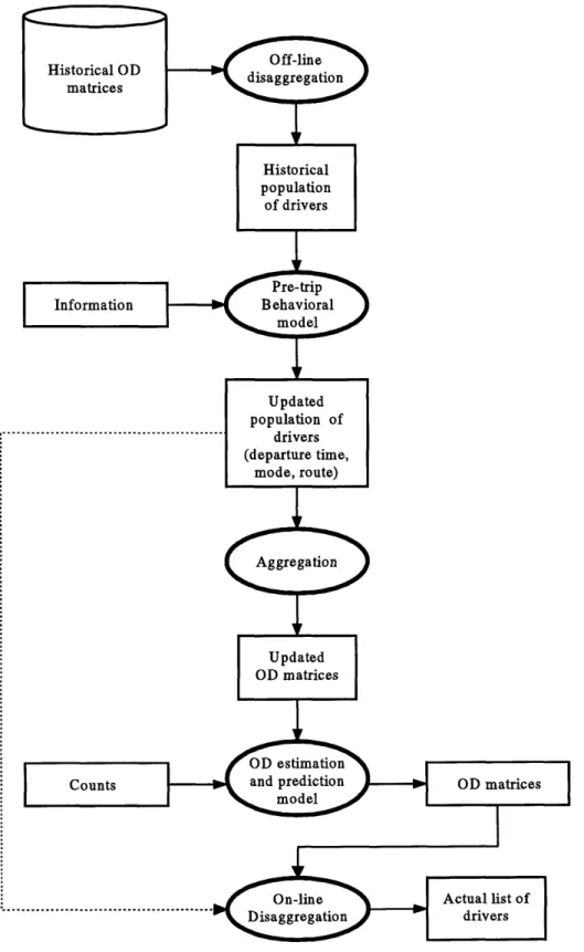
The overall structure of the proposed pre-trip demand simulator is presented in Figure 3.

Figure 3. Pre-trip Demand Simulator

(27)

,---The functionality of the pre-trip demand simulator can be separated in two main functions:

* Travel behavior update in response to information, and * Dynamic OD estimation and prediction.

The travel behavior model is disaggregate and is applied on individual drivers. On the other hand, historical demand is available as aggregate OD matrices. In order to be able to use the disaggregate behavioral model, the demand simulator transforms the aggregate OD matrices into a disaggregate population of drivers, upon which the behavioral model is applied. The off-line disaggregation is responsible for this. The behavioral model then updates the travel choices of each traveler, using the available real time information to determine if they will stick to their initial travel pattern or they will change departure time, mode or route, including canceling their trip altogether. After the travel behavior of each driver has been updated to reflect the available information and guidance, the aggregate OD estimation model is applied on the updated population of drivers. Therefore, the population of drivers is aggregated to a set of updated OD matrices (one OD matrix is generated for each departure time interval).

At this stage, the historical OD matrices have been updated to reflect the response of the drivers to available real-time information. If this step had been omitted, then the simulator would ignore significant information that could potentially affect its success in estimating current OD matrices. After the behavioral update has been completed, the OD estimation model accepts the updated OD matrices as input and uses traffic counts from the surveillance system to estimate aggregate demand for the current interval in the form of an estimated OD matrix. The OD prediction model makes an assumption about time evolution of demand to predict OD matrices for a given number of future intervals.

The pre-trip demand simulator is designed with the capability to be used in a wide range of applications, as discussed in Section 1.3. Depending on the nature and the requirements of each application, the output of the module can be either:

* Aggregate demand, or * Disaggregate demand.

If aggregate demand is required as output, then no further operation is performed and the estimated and predicted OD matrices are the desired output. On the other hand, if disaggregate demand is required, then the estimated and predicted OD matrices are disaggregated to a list of drivers by an additional on-line disaggregation component. This

(28)

procedure uses the previously generated updated population of drivers as basis, and adds or removes drivers to reflect the OD estimation results. For example, if for a given OD pair the final estimated flow is 100 drivers, but in the updated population of drivers there are only 95, then five additional drivers will be generated in the same fashion that was used in the off-line disaggregation. Similarly, if there are 105 drivers in the updated population for that OD pair and time interval, then five of them will be selected, using Monte Carlo simulation, and removed from the population of drivers.

In the remainder of the chapter, the variables and parameters that are used in the simulator are defined and the time discretization and the choice set generation procedure are presented. Furthermore, the major components of the demand simulator are described in more detail, including the models and the algorithms that are used.

3.2 Variable and Parameter Definition

The pre-trip demand simulator uses a number of variables and parameters in the specifications of the disaggregate travel behavior models. These are presented in this section. The variables are summarized in Table 1.

In the following definitions superscript H refers to historical information, whereas superscript I refers to information provided by the information system. Subscript h refers to departure time interval h and subscript p refers to path p. Finally, prime (') is used to denote habitual, e.g. h'is the habitual departure time interval and p'is the habitual path.

Abbreviation H tt,

tt I

I tthp' I tth'p I tth'p' dth Variable

historical travel time for departure time interval h and path p historical travel time for other (than car) mode

travel time provided by the information system for departure time h and path p

travel time provided by the information system for departure time h and habitual path p'

travel time provided by the information system for habitual departure time h' and path p

travel time provided by the information system for habitual departure time h' and habitual path p'

(29)

I

athp arrival time of traveler departing in interval h on path p

athI arrival time of traveler departing in habitual interval h' on path p

athp, arrival time of traveler departing in interval h on habitual path p'

athp, _{arrival time of traveler departing in habitual interval h' on habitual}

path p'

H

ath p' habitual arrival time for traveler with habitual interval h' and path p'

T time that the information is sent to the traveler

VOTIo low value of time indicator

VOTd medium value of time indicator

VOThi high value of time indicator

Pw work as trip purpose (0-1 dummy variable)

PI leisure as trip purpose (0-1 dummy variable)

CF, commonality factor for path p

l,

length of path p

w, length of path p in highway

cp out-of-pocket monetary cost for path p

s, number of signalized intersections in path p

fp number of left turns on current path p

Table 1. List of variables for travel behavior models

The historical travel time tt~ is the average travel time observed for departure time interval h and path p over prior observations. The variable ttmH is the minimum from the historical travel times for all alternative non-driving modes. In other words, this is assumed to be the historical travel time of the alternative mode that a driver is considering. The travel time tthp is the travel time that the information system gives to drivers departing during interval h on route p. Variables tt., ttP, and ttu can be interpreted similarly.

The departure time dth is the actual departure time of a traveler departing in interval h. It is calculated by assuming uniform departure rate for the departure time

(30)

interval and using Monte Carlo distribution to draw the exact departure time within that interval. The arrival time of a driver departing in departure time interval h on path p is given by atp = dth + ttp. When the habitual departure time h' or habitual path p' are considered, the arrival time variable becomes at, at and at accordingly. Similarly, the habitual arrival time for a driver departing in departure time interval h on path p is given by athp'n = dtht + tthp.

The time that the traveler receives the information is denoted by T. There are also three indicator variables VOTIo, VOTmd, VOThi to reflect the value of time of the driver (low, medium, or high). Only one of these variables is equal to one for each individual, while the other two are zero. In addition, there are two 0-1 dummy variables to capture the trip purpose of the driver (work or leisure). The variable that corresponds to other trips purposes is used as reference and, therefore, is not included in the utility functions. The selection of the referent alternative has no effect of the outcome of the model. Changes in the referent only shift the values of the estimated constants, preserving their difference.

The commonality factor CF, (Cascetta et al., 1996) for path p is an additional "cost" attribute in the utility of a logit model, which deals with the similarities among overlapping paths (this will be described in Section 3.5.1). The commonality factor does not affect travel behavior. Its role in the model is to overcome the limitation of the IIA property. The length of path p, lp, the length of path p that is on highways, wp, the monetary cost of path p, cp, the number of signalized intersections in path p, sp, and the number of left turns in path p, fp, are attributes of the paths. The same variables with subscript p' are used to refer to the habitual path.

Functions of the aforementioned variables appear in the models, as well. The variable dth' - T is used to describe how early the traveler receives the information (how

much earlier than the habitual departure time). For example, information received two hours before the habitual departure time may not be as relevant as information received 15 minutes before. In the specification of the utilities this variable appears as

max(dth' - T,0). This is to ensure that the variable takes a value of zero if the information

comes after the departure (since then it is not relevant for pre-trip decisions).

The variables at ' _at and at - Hath-p express the deviation in the arrival

time of the traveler departing at departure time interval h on path p, relative to the habitual arrival time for the habitual arrival time and path. This, in association with the possible early or late arrival penalty, captures the effect of arrival time variations in the

(31)

travelers' decisions. The variables are introduced in the specification of the utilities as the following terms:

* max(ath, p'- athp,0), and

* max(at - atp,0).

The first term captures the early arrival. It is zero if the arrival time is later than the habitual arrival time (i.e. athp < athp -the user is expected to be late). Otherwise, it is equal to the amount of time that the driver is expected to be early. Similarly, the second term captures the late arrival. It is zero if the expected arrival time is earlier than the habitual arrival time (i.e. at hp, > ath - the user is expected to be early). Otherwise, it is equal to the amount of time that the driver is expected to be late. The use of two such variables allows for designing different penalties for late and early arrivals. Terms max(ath - at , 0), max(at -at ,), max ath'p atp',0), and

max(athp- ath.p,O) are used similarly in the utility functions.

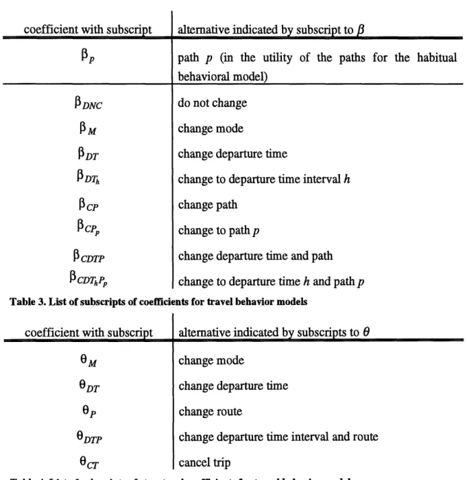
Tables 2, 3, and 4 present the coefficients of the models. The coefficients 8 and the structural coefficients 0 appear in the utility and probability equations as well. There are superscripts and subscripts to these parameters that need to be defined. Superscripts specify the model to which the coefficients refer to. These superscripts are defined in Table 1. Some # coefficients are specific to the corresponding alternative, denoted by the appropriate subscript. These subscripts are defined in Table 3. Furthermore, all of these variables are associated with a numerical identifier, ranging from 0 to 14. Finally, the structural coefficients, 0, have a subscript that defines the alternative they are associated with. These subscripts are presented in Table 4.

Coefficient with superscript

ph

od

OP

model indicated by superscript habitual behavior

behavior based on descriptive information behavior based on prescriptive information

(32)

alternative indicated by subscript to . pP DNC PDT fDTh CP cPP CDTP OCDThPp

Table 3. List of subscripts of coefficients for travel behavior models

coefficient with subscript

0 _M

0_DT

Op

OcCT

alternative indicated by subscripts to 9 change mode

change departure time change route

change departure time interval and route cancel trip

Table 4. List of subscripts of structural coefficients for travel behavior models

3.3 Time Discretization

Time is a very important dimension in simulation environments. The demand simulator is a discrete step simulator, i.e. the state of the system is updated in a series of steps, each corresponding to some fixed time interval (Lerman, 1993). The demand simulator uses two such time discretizations intervals:

* Departure time interval, and * Estimation interval.

path p (in the utility of the paths for the habitual behavioral model)

do not change change mode

change departure time

change to departure time interval h change path

change to path p

change departure time and path change to departure time h and path p coefficient with subscript

(33)

The departure time choice of individual drivers is modeled as a discrete choice. Therefore, a time discretization is necessary in order to define the choice set. This time interval needs to be small enough in order to realistically represent the drivers' change in departure time in response to information. Nevertheless, very small departure time intervals would increase the computational strain and the data requirements of the simulator. Therefore, in order to make a decision for the departure time interval length, this tradeoff should be examined and the length of the departure time interval should be selected based on the needs of the application.

Similarly, the OD estimation is performed for discrete intervals of time. Therefore, an interval that refers to the time period for which the demand is estimated is also necessary. The selection of the length of the estimation time interval depends on the application. As it will be explained in Sections 3.5 and 3.7, the two time intervals do not need to coincide. In such a case, a procedure that maps one time discretization into the

other is applied (see sections 3.5 and 3.7).

3.4 Choice Set Generation

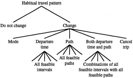
The behavioral models that are incorporated in the demand simulator are discrete choice models and require that the individual drivers' choice sets are explicitly specified. The travel decisions that the demand simulator considers are:

* Mode choice,

* Departure time choice, * Route choice, and * Trip cancellation.

Regarding mode, only the decision whether to drive or switch to public transit is considered and, therefore, the alternatives are clear. Since the demand simulator focuses on private transportation, only travelers switching from the automobile to transit are captured. Similarly, for the trip cancellation choice, the driver may choose whether to make the trip or not. Regarding departure time choice, the feasibility of the time intervals is bounded by the decision time, since an individual can not decide to depart earlier than the decision time. Since the habitual departure time interval is captured by the do not

change alternative, the departure times that are considered for the change departure time

alternatives do not include it. In the case of path choice, the choice set of an individual is considered to comprise from all paths connecting the origin and destination of interest. Again, the change path alternatives do not include the habitual path, since it is covered by

(34)

the do not change alternative. In the case of both departure time and path change, the choice set is comprised from all possible combinations of the time intervals in the departure time choice set with the paths in the path choice set. The only combinations that are excluded from the choice set are those that include the habitual departure time, the habitual path, or both.

In practical applications, it may be desirable to keep the number of alternatives to a reasonable size. In this case, the choice set can be filtered to exclude paths and departure time intervals that are very unlikely to be selected. Paths with very high travel times can be removed from the choice set, since they are unlikely to be chosen. Similarly, departure time intervals that are a lot later than the habitual departure time may also be safely removed from the choice set, based on the assumption that the travelers need to complete their trip within some time frame. Nevertheless, one needs to be cautious in such an elimination procedure, in order not to exclude alternatives that may become

attractive under certain conditions, such as an incident on a generally preferable route.

3.5 Off-line Disaggregation

The role of the off-line disaggregation component is to generate a population of drivers from the historical OD matrices. A number of socioeconomic characteristics, such as value of time, and trip characteristics, such as trip purpose, are generated and assigned to each driver. Origin, destination, departure time interval and mode are assigned to the drivers using information from the OD matrices. The origin and the destination come from the particular OD pair for which the driver is generated, the departure time interval is the interval to which the OD matrix corresponds and the mode is by default the car (since it is assumed that the OD matrices contain only car trips). Furthermore, a habitual behavior model is applied to each driver in order to generate habitual travel behavior based on historical information. This is presented in sections 3.5.1 and 3.5.2. Section 3.5.3 presents the entire off-line disaggregation algorithm.

3.5.1 Habitual Route Model Structure

The behavioral model that is used to provide choice probabilities for each path is the C-logit model, a modified multinomial logit (MNL) model, proposed by Cascetta (1993). The model specification of the C-logit is that of a MNL with a modified utility to account for overlapping paths. The model overcomes the main shortcoming of MNL where unrealistic choice probabilities result for paths sharing a number of links. For example, consider the simple network represented in Figure 4. This network is composed

(35)

from three nodes, A, B and C, and four links. There are three alternative routes connecting A and B. Assuming equal utility for the three alternative routes, a logit model would result in equal choice probabilities, 0.333, for each alternative route. This is not realistic, since paths 1 and 2 are practically identical. In the C-logit model this is captured by the introduction of an additional "cost" parameter in the utility specification.

1

C

A B

2

3

Figure 4. Simple road network with overlapping paths

The model requires explicit path enumeration. The structure of the model is presented in Figure 5.

Path A Path B ... Path N

Figure 5. Structure of the C-logit model

The choice alternatives are the paths that connect the origin and the destination of each driver and are included in the choice set.

In the C-logit model, the effect of overlapping paths is taken into account by the introduction of a term called "commonality factor" in the utility function. The commonality factor can be interpreted as the degree of overlapping of a path with the other paths in the choice set of the individual. The function of the commonality factor is to decrease the utility of heavily overlapping paths by introducing an additional "cost" in the utility of the paths, which is higher for overlapping paths. The reader is referred to Cascetta et al. (1996) for a more complete presentation of the commonality factor. In this reference, one can find alternative specifications, as well as a behavioral interpretation of the commonality factor. For the purposes of this application, the following specification has been selected:

CFp = In XcOpNj ₍₁₎

jE p

where: