The consequences of Fiscal Episodes in OECD Countries for Aid Supply

HAL Id: halshs-00613161

https://halshs.archives-ouvertes.fr/halshs-00613161

Preprint submitted on 3 Aug 2011

HAL is a multi-disciplinary open access archive for the deposit and dissemination of sci-entific research documents, whether they are pub-lished or not. The documents may come from teaching and research institutions in France or abroad, or from public or private research centers.

L’archive ouverte pluridisciplinaire HAL, est destinée au dépôt et à la diffusion de documents scientifiques de niveau recherche, publiés ou non, émanant des établissements d’enseignement et de recherche français ou étrangers, des laboratoires publics ou privés.

The consequences of Fiscal Episodes in OECD Countries

for Aid Supply

Sèna Kimm Gnangnon

To cite this version:

Sèna Kimm Gnangnon. The consequences of Fiscal Episodes in OECD Countries for Aid Supply. 2011. �halshs-00613161�

CERDI, Etudes et Documents, E 2011.22 1

C E N T R E D'E T U D E S E T D E R E C H E R C H E S S U R L E D E V E L O P P E M E N T I N T E R N A T I O N A L

Document de travail de la série Etudes et Documents

E 2011.22

The consequences of Fiscal Episodes in OECD Countries

for Aid Supply

Kimm Gnangnon

June 2011

C E R D I

65 BD.F. MITTERRAND

63000 CLERMONT FERRAND - FRANCE TÉL.0473177400

FAX 0473177428 www.cerdi.org

2

L' auteur

Kimm GNANGNON

PhD student, Clermont Université, Université d’Auvergne, CNRS, UMR 6587, Centre d’Etudes et de Recherches sur le Développement International (CERDI), F-63009 Clermont-Ferrand, France Email : kgnangnon@yahoo.fr

Corresponding author: K. GNANGNON, CERDI-CNRS. Email : kgnangnon@yahoo.fr

La série des Etudes et Documents du CERDI est consultable sur le site :

http://www.cerdi.org/ed

Directeur de la publication : Patrick Plane

Directeur de la rédaction : Catherine Araujo Bonjean Responsable d’édition : Annie Cohade

ISSN : 2114-7957

Avertissement :

Les commentaires et analyses développés n’engagent que leurs auteurs qui restent seuls responsables des erreurs et insuffisances.

3 Abstract

This paper contributes to the established literature both on the side of fiscal consolidation (for e.g. Alesina and Perotti 1995; Alesina et al. 2010) and that of aid supplies (for e.g. Mosley 1985; Faini, 2006) by investigating the effects of fiscal episodes in OECD donor countries on their aid effort vis-à-vis the developing countries. We use descriptive statistics provided by Alesina and Ardagna (2010) on episodes of fiscal consolidation and stimuli in OECD countries and regression models to perform this analysis. The study is performed on a sample of 19 OECD DAC countries as well as on sub-samples for robustness check and over the period 1970-2007. Overall, the results suggest that the episodes of fiscal consolidation and the size of these fiscal austerity policies in OECD DAC countries lead to the curtailment of aid effort. Whilst during periods of fiscal expansion, aid expenditures increase, the size of these fiscal expansion policies may have an opposite effect.

The fiscal austerity measures currently adopted by OECD DAC countries are likely to result in aid shortfalls to developing countries, with these effects likely be higher in the “Like-minded Donor countries”.

JEL Classification: F35, E62, H62, H85

Key Words: Foreign Aid, Fiscal consolidation, Fiscal stimuli.

Acknowledgements

I would like to thank Mr Jean-François Brun, Mr Gerard Chambas as well as the participants of the ANR seminar for their helpful comments and suggestions. Thanks also to Mr Alberto Alesina and Ms Silvia Ardagna for generously sharing their dataset used in Alesina and Ardagna (2010). I am also grateful to the “Agence Nationale pour la Recherche –France” for its financial assistance. All errors are the responsibility of the author.

4

1. Introduction

In response to the largest post-war recession, OECD governments have run up record peacetime budget deficits. The recent financial crisis has constrained them to embark on major fiscal stimulus in order to rescue their financial institutions and the ensuing Great Recession. As a result, budget deficits and government debt soared, leading to a substantial deterioration of their fiscal situations.

Actions to design and implement “exits” from fiscal stimulus become imperative and prompt countries to adopt fiscal consolidation measures in order to make their public finances sustainable. Furthermore, population ageing could create on the medium to long-run pressures on public finances that adds to the fiscal consolidation effort.

While there is an ongoing debate about the best balance between cuts in expenditure and rises in tax during episodes of fiscal consolidation, several empirical studies (Alesina and Perotti (1995, 1997a, 1998), McDermott and Wescott (1996), IMF (1996), OECD (1997) and Perotti (1997), Alesina and Ardagna 1998, Ardagna 2007, Alesina and Ardagna 2010, IMF 2010) tend to convey the same message: “fiscal adjustments which rely primarily on spending cuts on transfers and the government wage bill have a better chance of being successful and are expansionary. By contrast, fiscal adjustments which rely primarily on tax increases and cuts in public investment tend not to last and are contractionary”. However, Heylen and Everaert (2000) empirically contest the result according to which current expenditures reductions are the best policy to get a successful fiscal consolidation.

On the side of fiscal expansions, Alesina and Perotti (1995a) find evidence that fiscal expansions typically occur through increases in expenditures. More recently, Alesina and Ardagna (2010) also find evidence that fiscal stimuli based on tax cuts are more likely to increase growth than those based upon spending increases.

In view of all these different empirical results, one can question whether fiscal episodes in donors’ governments do not affect aid supply. Indeed, it is likely that during fiscal consolidation episodes where government expenditures will likely be curtailed, development aid supplies by the OECD DAC countries that constitute a category of government expenditures will also be reduced. Similarly, we can also expect donors’ governments to increase aid expenditures during fiscal stimuli years as the other categories of government spending rise. At the same time, these OECD DAC countries have committed either individually or collectively (through international meetings) to achieve a target level of aid flows granted to developing countries,

5 commitments that have been renewed at the Gleneagles summit. In 2010, the OECD has estimated that at least USD 10-15 billion must still be added to the forward spending plans if donors, are to meet their 2010’s commitments. However, during the same year, the OECD has communicated (on 14th April 2010) that Africa will not likely receive more than the USD 11 billion over the USD 25 billion promised at the Gleneagles summit, due to the adjustment measures adopted by the country members in response to the recent financial and economic crisis.

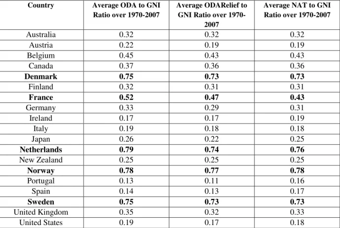
The figures1 _{reported in table 1 show evidence that over the period 1970-2007, on} average, only four countries (Netherlands, Norway, Sweden and Denmark) have achieved, even exceed the international ODA target of 0.7% of GNI. These results suggest that several variables affect the decisions of donors to supply aid and may explain why many of them do not fulfil their ODA commitments. In this paper, we explore the role of fiscal episodes in explaining this phenomenon.

As we will see later, the empirical literature has already established that recipient-country characteristics such as income level, population, and political system (see for e.g. Alesina and Dollar 2000; Dollar and Levin 2006) affect aid inflows. However, the empirical literature on the donor-side’s determinants of aid, especially the one that focuses on the fiscal variables remains short and inconclusive. For example, Faini (2006) finds evidence that higher budget deficit and higher stock of public debt reduce aid, whereas Round and Odedokun (2004) and Boschini and Olofsgard (2007) find no significant relationship between deficits and aid provision. Moreover, none of these studies explore the effects that the fiscal episodes in donor countries may have on aid provision.

In this paper, we investigate how donors behave in terms of aid supplies during the fiscal episodes. In other words, we explore the effects of fiscal consolidation and stimuli episodes in OECD donor countries’ aid supplies, irrespective of their effect on per capita income and other economic and political variables. We follow the literature on fiscal episodes and use descriptive statistics and regression models to perform this analysis.

The paper is structured as follows: in the next section (II), we provide a literature survey on the topic. We then explain how the fiscal episodes in OECD countries are determined (III). In section IV, we present our empirical model. Section V discusses the data

1 _{Figures are computed by the Author using the OECD’s Statistics on Overseas Development} Assistance (ODA) and Gross National Income (GNI).

6 and econometric methodology and section VI presents empirical results. The last section concludes.

2. Literature Review

Several, though controversial studies have been conducted on the supply of foreign aid, with most of them relying on how recipients’ characteristics affect aid delivery. These studies examine the potential factors and motivations behind the supply of aid by answering questions such as: Who received aid? How much is received and for what kinds of activities? Many of them find evidence that donors’ political, economic and strategic interests appear to dominate altruistic and development-centered motivations in their foreign aid programs. For example, Alesina and Dollar (2000) use bilateral data on DAC countries over 1970-1994 and find evidence that factors such as colonial ties and strategic considerations (i.e. proxied by the degree of correlation in the donor and recipient countries’ voting records at the UN) are among the factors that could influence the flow of bilateral aid.

However, limited studies have dealt with the supply side determinants of aid flows from the donor’s perspective (that is, the determinants of “aid effort” or “aid generosity”). For example, the focus of these studies on how macroeconomic variables (and especially fiscal policy ones) can affect theoretically and empirically aid generosity remains scarce: Beenstock 1980; Mosley 1985; Faini (2006) and more recently Sam (2011) have been the few authors that explore both theoretically and empirically the determinants of aid supplies. We present here the theoretical and empirical literature on this issue.

2.1 The theoretical literature review on the determinants of aid supply

Beenstock (1980) developed a statistical model that sheds light on the political decision-making process regarding the allocation of aid by OECD countries and where the latter depends among others on the level of unemployment, the budget balance, the balance of payments, the Gross National Product, the level of population. After estimating his model on alternatively 8 (Canada, France, Germany, Japan, UK, US, the Netherlands and Sweden) and 6 countries (Canada, France, Germany, Japan, UK, US) over the period 1960-1976 (T=17 Years), he finds evidence that Aid flows are negatively and significantly affected by the unemployment level, the population level, and the net budget surplus, whereas it is positively affected by the balance-of-payments, the GNP, and a time trend.

The theoretical model on Aid flows determinants developed by Mosley (1985) relies on the Breton (1974)’s approach to market adjustment in the case of goods provided by the

7 public sector. He treats aid as a public good for which there is a market, albeit highly an imperfect one.

Assuming that aid determinants rest on a demand and a supply function of aid, he shows theoretically that the adjustment of the supply function to the demand function of aid leads to an equation where aid flows depend on the unemployment, the Government Budget deficit, the aid disbursement of all OECD countries other than country i, the level of per capita income in country i in relation to per capita of other OECD countries and an Indicator of Aid quality. This equation is estimated for each country separately as well as on pooled regression. The sample covers 9 OECD countries (Canada, France, West Germany, Japan, Netherlands, Norway, Sweden, USA and U.K) over the period 1961-1979. Using OLS technique country by country, he concludes among other variables for a positive and significant effect of the central government budget deficit on aid flows for Netherlands and United Kingdom, whereas the effect is mixed (either positive or negative) but not statistically significant for the other countries.

Faini (2006) also explores through a theoretical model the links between fiscal policy in donors’countries and their aid effort. He develops a simple model and obtained that the OECD Donors’ aid effort depends on the budgetary conditions (the primary surplus and the stock of public debt), on the political orientation of the government, the output gap, and the one-year lagged value of the aid effort. This model is estimated with the dependent variable proxied alternatively by the net official ODA; the total official flows and the Roodman’s Net Aid transfers measure. The sample covers 15 donor countries over the period 1980-2004. The use of fixed-effects method leads him to conclude that an increase in the budget deficit or in the stock of debt leads to a severe decline of the development assistance.

The last theoretical model is that of Sam (2011) who examines the aid expenditures response to banking crises in donor countries. He develops and estimates a model of long-run and short-run determinants of aid supply. Using the two-step of Engle and Granger’s method with fixed effects, he observed that bilateral aid supplies2 are positively driven in the long-run by government saving and government expenditures (both in percent of GDP). Moreover, government spending (as a percentage of GDP) drive positively aid disbursements on the short-run.

2 _{Total bilateral aid is here the net bilateral aid disbursement minus debt relief which excludes} disbursements to multilateral organizations but includes support to NGOs and international private organizations) over the period 1960-2009.

8

2.2 The review of the empirical literature on the determinants of aid

generosity

Besides the theoretical models described above, several other empirical studies have been conducted on this topic.

Round and Odedokun (2004) investigating the decline in aid flows over the period 1970-2000 on a sample of all 22 DAC countries, have looked at the determinants of gross disbursements of ODA loans and grants, as a proxy of aid generosity. By controlling for other political and non-political factors (per capita income, peer pressure, the number of checks and balances, polarization and fractionalization within the government, a time trend and the political orientation) they do not find a significant effect of fiscal balance on aid effort.

Bertoli et al. (2008) have concentrated their study on the determinants of aid effort (proxied by the net aid disbursements, net of debt relief, as share of GDP) for all of the 22 OECD DAC countries over the period 1973-2002, with a particular focus on the Italian case for a comparison purpose. In employing fixed effects estimation technique and controlling for other political and non-political factors, they observe that the fiscal deficit exerts a positive effect on aid generosity.

Mendoza et al. (2009) investigate in the wake of the global financial crisis whether economic and financial conditions are negatively linked to official development assistance (both bilateral ODA and total ODA) provided by the USA. Focusing on the period 1967-2007, they show evidence that among other regressors, tax revenues do not affect significantly both bilateral and total US ODA.

Dang et al. (2010) investigate the effects of banking crisis on a sample of 24 donor countries over the period 1977-2007. They use two indicators of aid: Net Aid disbursements and Net Aid Transfers and find evidence that banking crisis exert severe negative effects on aid supplies, with these effects diminishing over time. The lagged budget surplus/deficit (in % of GDP) in the donor’s countries adversely influences aid flows, suggesting that the budget surplus is achieved by cutting aid along with many other spending categories.

Mold et al. (2010) also explore empirically the determinants of net bilateral ODA on a panel of all 22 DAC countries over the period 1960-2007. By employing the System-GMM estimator (Blundell and Blond, 1998) and fixed effects, they conclude that the scope for aid allocations are larger when fiscal circumstances allow it, and that geopolitical and political purposes are important in aid disbursements.

9 Chong and Gradstein (2002) examine the determinants of foreign aid with respect to the donors. Applying both fixed-effects panel data and Arellano-Bond dynamic estimator techniques, they conclude on a sample of 22 DAC countries over the period 1973-2002 that as tax revenues increase, aid effort rise.

Other studies have focused more on the political determinants of aid supplies.

Boschini and Olofsgard (2007) use a dynamic econometric methodology (both fixed effects and GMM procedure) on a panel of 17 donor’s countries over the period 1970-1997 to test whether the sizeable reduction in aggregate level of aid flows in the 1990’s was due to the end of the Cold war. As a control variable, fiscal balance appears to not exert a significant effect on aid supplied by donors. Dustin Tingley (2010) has broken out foreign aid by different categories (e.g., low-income versus high-income developing countries) and channels (bilateral versus multilateral) to examine how domestic political and economic environment influence the support for foreign aid. Using two main political variables (a measure of the government ideological orientation and changes in welfare state institutions proxied by the time-varying “generosity” indicator calculated by Scruggs (2006)), he concludes that as governments become more conservative, their aid effort is likely to fall. Moreover, changes in welfare state institutions exert positive effects on total and multilateral aid as well as aid to LDC/OLIC (Least Developed Countries/Other Low-Income Countries), but no significant effect on LMIC/OMIC (Low-Middle Income Countries/Other Middle Income Countries).

Overall, we can infer from this empirical literature that “the fiscal determinants of aid supply contradict one another sufficiently so that there is no trenchant evidence on the relationship between fiscal policy and aid flows”.

Our purpose in the following sections is to understand how fiscal variables, especially fiscal episodes, namely fiscal consolidation and fiscal stimuli episodes as well as their size in donor countries affect the aid expenditures toward developing countries. The next section will consider how these episodes fiscal in OECD countries are determined.

3. The determination of Fiscal episodes in OECD Countries

The choice of the approach to measure the fiscal episodes is a critical point when assessing their effects on Aid supplies.

The empirical literature provides several definitions for timing fiscal contractions and stimuli (expansion) with most of them relying on the structural budget balance concept, the balance that results from intentional actions of policymakers.

10 Fiscal episodes (consolidations and stimuli) result from the attempts of the governments to change the budgetary position of the government: fiscal consolidations or stabilizations aim at adopting discretionary fiscal policies which cut budget deficits whilst fiscal stimuli consist of discretionary fiscal policy that increase budget deficits. To identify fiscal consolidation episodes, we need to compute a measure of fiscal impulse. The Fiscal Impulse is the discretionary change in budgetary position and can be measured as the difference between the actual budgetary position and what would prevail under a benchmark cyclical situation (Alesina and Perotti, 1995a).

As mentioned by Alesina and Perotti (1995a), the use of the discretionary changes in fiscal policy indicator means eliminating from the budget balance two components: the interest payments, which cannot be directly influenced by government’s policies and the cyclical component of the budget.

The first adjustment implies the use of the primary surplus (or deficit), whilst the second correction is more problematic. This is why there exists several ways on the empirical literature to deal with this issue:

- one possibility is to ignore the existence of the cyclical component in the primary budget balance and consider the change in primary deficit as the measure of fiscal impulse.

-the second option is to use the cyclically adjusted budget deficits provided by the OECD or the IMF that rely upon somewhat arbitrary measures of “potential output” and base years.

- the last option is the one suggested by Blanchard (1993). This approach is more attractive to the extent that it does not require a measure of potential output for computing the primary surplus (deficit) corrected for cyclical components. This measure consists of calculating how the budget balance would be in a certain year, if unemployment had not changed from the previous year: this cyclical adjustment is an attempt to eliminate from the budget balance, changes in taxes and transfers induced by changes in unemployment, when tax-transfers laws remained unchanged.

Once calculating the fiscal impulse measure, we need a rule to identify the fiscal episodes (fiscal consolidations and fiscal stimuli periods). The criteria used in the existing literature to identify these episodes differ slightly from paper to paper. In this paper, we apply the original Alesina and Perotti (1995)’s definitions, re-employ recently in Ardagna and Alesina (2010) and also widely used in practice. According to those definitions,

11 - “A period of fiscal adjustment is a year in which the cyclically adjusted primary

balance improves by at least 1.5 percent of GDP”.

- “A period of fiscal stimulus is a year in which the cyclically adjusted primary

balance deteriorates by at least 1.5 percent of GDP”.

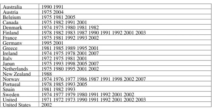
Accordingly, we use the episodes of fiscal adjustments and stimuli identified by Ardagna and Alesina (2010) to examine their effects on aid efforts: the authors focus upon a sample of 21 OECD countries with data spanning over 1970-2007. The countries included in their sample are: Australia, Austria, Belgium, Canada, Denmark, Finland, France, Germany, Greece, Ireland, Italy, Japan, Netherlands, New Zealand, Norway, Portugal, Spain, Sweden, Switzerland, United Kingdom, and United States. However, in our database, we exclude “Greece and Switzerland” because these countries have significantly short panels, though our results do not change if we include them.

Relying on large changes in fiscal policy stance, especially on the reductions and increases of budget deficits, Alesina and Ardagna (2010) use the Blanchard (1993)’s indicator of fiscal impulse (changes in the cyclically adjusted primary balance) to identify the fiscal episodes. Overall, they identify 107 periods of fiscal adjustments, 65 last only for one period, while the rest are multiperiods adjustments and 91 periods of fiscal stimuli with 52 lasting on year, the remaining are multiperiods. The table 2a and table 2b list respectively the episodes (years) of fiscal consolidation and fiscal stimuli identified by Alesina and Ardagna (2010).

To have a first look at the response of the Aid flows to the episodes (“before”, “during” and “after”) of fiscal consolidations and stimuli, we regress the “Aid variables” on dummy indicators for periods “before”, “during” and “after”. Thus, we estimate the following equations:

, 1 2 1 2 1 2 ,

i t i i t

Aid =α +β Beforefa+β Beforefs+λEpFA+λ EpFS+γ Afterfa+γ Afterfs+ε where the “Aid variable” is alternatively the Net Aid disbursements in percent of GDP (ODA), the Net Aid disbursements in percent of GDP from which debt forgiveness in percent of GDP is excluded (ODARelief) and the Net Aid Transfers (Roodman 2009) in percent of GDP (NAT) (these “Aid” variables are described further in the section IV); i denotes the country’s index: i = 1,..,19 and t denotes the time period index: t= 1970,...,2007.

β

₁,

β

₂,

λ

₁,

λ

₂,

1

12 “Beforefa “ and “Beforefs” are dummy variables taking the value of “1” the year before the fiscal episode starts in a donor country and “0” otherwise, for respectively episodes of fiscal adjustments (consolidations) and stimuli (expansion).

“Afterfa” and “Afterfs” are dummy variables that take the value of “1” the year after the last year of the fiscal episode in a donor country (i.e. for example, if a fiscal episode lasts 4 years, we associate the value “1” to the fifth year), and “0” otherwise for respectively episodes of fiscal adjustments (consolidations) and stimuli (expansion).

“EpFA” and “EpFS” are the variables indicating respectively the episodes of fiscal consolidations and fiscal stimuli.

We use as estimation technique the panel fixed effects method3. The results (in table 3 of the Appendix) of the estimations indicate that one year after the fiscal consolidation, aid declines significantly, irrespective of the “Aid variable” used. For the other variables of the model, we do not find a significant effect; this may be because we have not controlled for other explanatory variables. However, it does not matter at this stage of the study, as the purpose here is to have a first idea of the effects of fiscal episodes on aid disbursements. The next section is devoted to the specification of the model.

4. Econometric Specification

4.1 The Model

We follow a general approach that consists of estimating some version of the following equation: A_{i t,} =α_iX_it+β_iZ_it+µ_i+η_t+ε_{i t,} (1)

where i denotes the countries (i = 1,..., 19) and t denotes years (t = 1970, ..., 2007) and : the dependent variableAi t, =(Aid GDP/ )i t, denotes the total Aid flows (bilateral and

multilateral) from the country i in year t. We use as our primarily dependent variable the net ODA disbursements of aid flows of each donor and for robustness check, both the Net ODA disbursements of aid flows net of debt forgiveness, in percent of GDP (ODARelief), and the Net Aid Transfers (NAT)’s measure of Roodman (2009), also as a percentage of GDP.

3_{Fixed effects model (FE) appears as the logical econometric specification for having a first} look on the effect of fiscal consolidation variables on aid disbursements. The reasons are very simple: first, Fixed effects allow us to capture unmeasured state-invariant factors influencing aid in percent of GDP. Second, the countries in our sample constitute, in principle, the whole population of the donor countries, so it is appropriate to treat the individual effects as fixed rather than random.

13 The vector X_{i t,} represents the Fiscal Episodes variables and include: the episodes of fiscal consolidation, the size of the fiscal consolidation, the episodes of fiscal stimuli and the size of fiscal stimuli. These variables are included in all our regressions.

The vector Zi t, comprises two kind of time-varying control variables derived from the

empirical literature:

- On one side, a set of time-varying control variables that are include in all regressions: the fiscal balance (in percent of GDP), the gross public debt as a percentage of GDP and the Output gap. These variables combined to the fiscal episodes variables form our baseline regression model.

- On the other side, a set of time-varying and non-varying control variables derived from the empirical literature are included once in the baseline model: the degree of trade openness; a variable capturing the ideological orientation of the government; the number of years since the fiscal consolidation has started in a donor country as well as its square; the number of years since the fiscal stimuli has started in a donor country as well as its square; the quality of bureaucracy; the quality of governance; the level of population; the real effective exchange rate; banking crises; the unemployment rate; the inflation rate; the cold war and the welfare state institutions.

i

µ

are donor fixed-effects that are incorporated in the model to capture the heterogeneity among countries as well as the likely importance of unobservable correlated with the error term in determining aid flows. The use of fixed effects

µ

_i in our regressions is dictated by several reasons: First, since our sample is composed of heterogeneous countries, there are likely state-invariant and unmeasured factors correlated with the error term in determining aid flows.

Second, the number of time periods is significantly higher than the dimension of our panel. Moreover, our macro panel contains, in principle, most countries of interest (representing the whole population of the OECD donor countries), and thus, will not likely be a random sample from a much larger universe of countries.

t

η

are year dummies and are included in all specifications to account for common shocks to aid volume in any given year.

The disturbance εi t, is assumed to be i.i.d. (0, 2 ε

σ ), that is, assumed not correlated with the explanatory variables of the model and, the normality of which is not required (Baltagi, 2002).

14 Should our supply equation of aid flows have a dynamic specification?

Wildavsky (1964) points out that current year’s spending in any public agency is predominantly influenced by the budget of the previous year. Mosley (1984) reinforces this argument by stressing that it is particular true for aid agencies, since aid projects often run over several years, with financial flows being committed already in year one.

To explore statistically this likely dynamic specification, we follow the procedure suggested by Maddala (1987) and Anderson and Hsiao (1982). This procedure described in the appendix, refers to a Wald test to study if the lagged dependent variables has a direct effect on the dependent variable, apart from the indirect influence generated by serial correlations of the errors. If this is the case, then the model is called “state-dependence” or “system dynamic” and if not, it is called “serial correlation” or “error dynamics”.

To perform the test, we use two lags of the dependent variable because additional lags appear not significant. The results are presented in Table 8 and are further interpreted in the section V. Accordingly, we estimate the previous described model specification with two lagged dependent variables. While it is well-known that the fixed-effects estimator generate biased results in a dynamic panel, Nickell (1981) proves that this bias decreases in the number of time periods and approaches zero as T (the time period) approaches infinity (the time dimension of the panel is large). Accordingly, as our time-dimension is T=38 and our cross-section dimension is N= 19, we choose to work with the fixed effects.

In the next section, we discuss the expected sign of the different regressors included in the model.

4.2 Discussion on the Expected signs of the variables

Episodes of fiscal consolidations: During the episodes of large fiscal consolidation,

governments tighten their budgets and reduce the high debt levels to make public finances sustainable. Therefore, we can expect governments to reduce several items of expenditure including spending on aid flows, despite their firm commitment to increase aid exports to recipient’s countries. However, as have mentioned Round and Odedokun (2004) - P306, since “aid can act as an immense foreign policy tool for donor governments, it is not a particular discretionary item in the budget”; thus, it may not be reduced even in deterioration of public finance situations. Although this argumentation runs contrary to the expectation of a procyclical pattern of foreign aid (Hallet, 2009), we can also expect aid expenditures to be protected during the episodes of fiscal consolidation. In other words, large Fiscal

15 consolidation can exert a positive effect on aid flows. In addition, we also assume the governments in face of several competing government expenditures to reduce several items, but maintain or increase aid exports for strategic or geopolitical reasons: aid could be protected even when spending is being constrained (Round and Odedokun 2004).

The Size of fiscal consolidation: the greater the size of tightening fiscal policy, the

higher the effect on aid supply. However, in reference to the hypotheses mentioned above, the size of fiscal consolidation may be ambiguous as the effect may be positive or negative on aid supplies, depending on policymakers’ preferences.

Episodes of fiscal stimuli: During large episodes of fiscal stimuli that aim to

stimulate the domestic activity, aid expenditures may decrease (this is considered as a discretionary component that is cut in favour of social and investment spending), increase as the other discretionary components of expenditures, or it may neither increase nor decrease.

Size of the fiscal stimuli: We expect a priori that a high level of the fiscal stimuli size

will lead to a rise of aid expenditures. However, for the reasons mentioned above, the effect may be neutral or, aid supplies may even decrease.

The Budget deficit and the public debt: As in Mosley (1985), Round and Odedokun

(2004), Faini (2006) and Bertoli et al. (2008), we hypothesize that the cases of weaker fiscal position characterized by larger budget deficits and high levels of public debt, will ceteris paribus lead to the reduction in the level of discretionary spending, especially that of aid flows – because of strong pressures to reduce deficits and public debt and preserve scarce foreign currency. In other words, a healthy fiscal position will be associated ceteris paribus with higher spending, including on Official Development Assistance. We also follow Bertoli et al. (2008) and hypothesize that “given the small volume of aid relative to GDP, it is the overall level of public expenditures rather than its allocation among different expenditures chapters that influences the volume of aid” (see also Faini, 2006).

In contrast to these hypothesis and in accord with Bertoli et al. (2008), we can also assume that weak budgetary positions – or significant debt overhang may not have a detrimental impact on foreign aid, provided that the governments adopts an accommodating attitude towards the fiscal disequilibria over the medium term.

16

Output Gap: The effect of the output gap (the difference between the maximum

output achievable and the actual level of output) can be either positive or negative as a positive output shock may not necessarily lead to higher aid expenditures.

The Number of fiscal consolidation episodes: We introduce a counter variable (in

replacement of the variable “Epfa”) (see also Dang et al. 2010 for the same procedure with regard to the “banking crisis variable”) in our model to capture the effects of fiscal consolidation: the “number of years of fiscal consolidation”. This variable records the number of years since the first year where a fiscal consolidation occurs, with the first year taking a value of “1” and the value “0” for all years subsequent to the fiscal consolidation end’s year. To allow the effect to diminish over time, we include this counter variable in both linear and square terms in the model. In other words, we expect a negative effect of the counter variable “number of years of fiscal consolidation” but a positive effect of its square terms.

The Number of fiscal stimuli episodes: the construction of this variable follows the

same procedure as for the variable “number of years of fiscal consolidation” with the difference here being that this variable records the number of years since the first year of the occurrence of a fiscal stimulus. This variable takes the value of “1” for the first year, “2” for the second year,..etc, and the value “0” for all years subsequent to the fiscal stimuli end’s year. To allow the effect to diminish over time, we also include this counter variable in both linear and square terms in the model. In other words, we expect a positive, neutral or even a negative effect of this counter variable.

Openness degree: We follow the empirical literature on aid determinants (Boschini

and Olofsgard 2007; Dang et al. 2009; Dustin Tingley, 2010 and Sam, 2011) and assume that donor countries relying more on trade may see foreign aid as a useful tool to promote trade and hence increase their aid effort. Thus, the measure of how exposed a country is to trade Openness is: (Exports + Imports)/GDP.

Ideological Orientation of the government: The empirical literature on aid supplies

has posited that ceteris paribus, right-wing regimes in donor countries exhibit lower aid supplies compared to left-wing governments. However, the influence of government’s

17 ideological orientation (social-democrat versus libertarian-conservative) on aid supplies remains not clear-cut on the basis of aggregate aid data. Indeed, conservative governments may allocate more aid to promote national commercial interests, while progressive governments provide a similar amount for altruistic reasons (Round and Odedokun 2004; Bertoli et al. 2008).

Real Effective Exchange Rate: It is expected that a depreciation of the real exchange

rate will improve the balance of payments and thus increase overseas development assistance.

Unemployment: Beenstock (1980) and Mosley (1985) mention that unemployment is

one of the most important explanatory variables apart from fiscal balance when explaining aid expenditures, as there may be obvious incentives to cut aid expenditures and redirect funds towards domestic expenditures in times of fiscal problems. Thus, we expect unemployment to reduce the level of aid supplied by the donors.

The quality of bureaucracy: This variable captures revisions of policy when

governments change. As a change in government tends to be traumatic in terms of policy formulation and day-today administrative functions, a strong quality of bureaucracy should minimize the revision of policy when governments change. Therefore, we can expect a stronger quality of bureaucracy to be associated with a higher level of aid disbursements by donors.

The quality of governance: It is another way of measuring the role of political factors

on aid supplies. The quality of governance is a composite index of corruption in government, bureaucratic quality, and the rule of law. We expect a better quality of governance in a donor’s country to be associated with higher aid supplies.

Banking crises: As we have observed above, a banking crisis in a donor country is

expected to lead to a reduction of aid flows irrespective of its effect on the other economic variables such as real GDP or government budget. Indeed according to Dang et al. (2010) Bank rescues and recapitalizations place massive new fiscal demands on the public sector; even if the government is eventually able to recoup many of the costs of these rescues through asset sales, the short-term effect is to worsen sharply the government’s cash flow.

18

Inflation: Greater economic difficulties (for instance, a high level of inflation with its

inducing macroeconomic instability effects) will lead to lower support for foreign aid programs. Thus, we expect a negative effect of this variable on aid supplies.

Real GDP per Capita: Aid over GDP is assumed to be a “superior good”, that is, the

ratio of aid over GDP is expected to increase as the per capita income raises.

Population: According to Round and Odedokun (2004), an increase in population size

is likely to be associated with greater population heterogeneity, loss of social cohesion and ceteris paribus, declining willingness to redistribute. There is a support to this hypothesis to the extent that within the DAC, the small countries – such as the Nordics – are more homogeneous and cohesive and have for long maintained an altruist and progressive attitude towards foreign aid.

Cold: This variable captures certain main miscellaneous qualitative time-related

factors that affect aid supplies. Indeed, the empirical literature highlights that aid has plummeted from the early 1990s due among others to the end of the cold war. Indeed, the emergence of Eastern European countries from the early 1990s creates a competition with the conventional developing countries for aid and provides a greater freedom to donors for reducing aid on the basis of concerns about governance issues, fact to which they had to turn a blind during a cold war era (see Round and Odedokun 2004; Hjertholm and White 2000).

Welfare institutions: Therien and Noel (2000) argue that the influence of partisanship

is indirect and operates through other policies like social-democratic welfare state institutions and social spending. Hence, the influence of political parties is only cumulative and operates indirectly through welfare institutions: the strong welfare institutions best explain foreign aid spending patterns. However, whereas Therien and Noel (2000) argue that welfare state institutions are relatively fixed, this argument has recently been disputed by scholars who find that the earlier measures are deceptively static (Allan and Scruggs, 2004). We follow Dustin Tingley (2010) and use the “generosity” measure of Scruggs (2006) which is a time-varying measure of state welfare institutions (changes in state welfare institutions).

19

5. The Data and the econometric methodology

5.1 The Data

We define and describe here the “Aid variable” as well as the “fiscal episodes variables” used in our model. The other explanatory variables are described in the table 4. The model is estimated on a sample of 19 countries, with data covering the period 1970-2007. Indeed, as previously mentioned, we consider the entire sample of Ardagna and Alesina (2010) but exclude “Greece and Switzerland” (see above for explanation).

5.1.1 The Dependent Variable: Aid data

In the empirical literature on the determinants of aid flows, several indicators of aid effort have been used: whereas some authors have used “aid as a percentage of GDP” (for instance, Bertoli et al. 2008; Faini, 2006), few studies have relied on using as dependent variable the overall aid (for instance Boschini and Olofsgard, 2007, Dang et al. 2009) and others have resorted to the use of (log of) aid per capita (see for instance, Frot, 2009).

For our main test, the dependent variable is net Aid flows data (as a percentage of GDP) which allows us to control for loans repayments. More particularly, we use the Net disbursements of Official Development Assistance (ODA)’s share of GDP. The latter comprises grants and loans with at least a grant’s element of 25%.

We then check for the robustness of our main results by considering additional variables of Aid effort: the Net Aid disbursements minus debt forgiveness (ODARelief) and the Net Aid Transfers (NAT), described by Roodman, (2009)4, both as a percentage of GDP. The Net Aid Transfers concept subtracts out repayments of principal as well as interest payments and cancellation of non-ODA loans (aka debt relief). This variable more closely approximates the current budgetary outlays associated with ODA.

5.1.2 The Fiscal Episodes Variables

Episodes of Fiscal Consolidation (and Stimuli): We use the variables constructed by

Ardagna and Alesina (2010) according to their definition of “episodes of fiscal adjustments and fiscal stimuli” (see above). These authors have focused on large changes of fiscal policy to identify the episodes of fiscal adjustments and stimuli of OECD Countries.

20 The previous definition selects 100 episodes of fiscal consolidation (13.8% of the observations in our sample) and 85 episodes of fiscal stimuli (11.8% of the observations in our sample) for 19 countries over the period 1970-2007.

The Size of Fiscal consolidation (and Stimuli): We follow the empirical literature on

fiscal episodes (that is, consolidation and stimulus) (see for example, Guichard, S. et al. 2007) and consider the size of fiscal consolidation (and Stimuli) as the change in the cyclically adjusted primary balance expressed in percent of GDP over the whole episode (last year of the episode minus the year before it starts). It is worth mentioning that the measure of the cyclically adjusted primary balance used here is the one computed by Ardagna and Alesina (2010).

The Number of years since the fiscal consolidation (stimuli) has started in a donor

country: these two variables are constructed following Dang at al. (2009)’s methodology

related to banking crisis (see above for the description of these variables).

5.2 The econometric methodology

In this part, we discuss the econometric technique suitable for estimating the effects of fiscal episodes on aid supplies. Consider the model (1) described above. We first impose the restrictions that

α

_i =

α

and

β

_i =β, for i = 1,..., 19.

Our baseline model specification is:

, 1 2 3 4 1 2

3 ,

i t it it it it it

it i t i t

A epfa Sizetight epfs Sizeloose Govnetlend Pubdebt

Outputgap

α

α

α

α

β

β

β

µ

η

ε

= + + + + +

+ + + + (2)

where Ai t, denotes ODA, ODARelief or NAT variables as previously defined; EpFA =

Episodes of Fiscal Consolidation (Adjustment); Sizetight = Size of fiscal consolidation;

EpFS = Episodes of Fiscal Stimuli (Expansion); Sizeloose = Size of fiscal expansion or

stimuli; Govnetlend = General government fiscal balances (Total Revenues minus Total Expenditures) in percent of GDP; Pubdebt = Gross Public Debt-to-GDP-ratio; Outputgap = the outputgap;

µ

i and

η

t are respectively country-specific effects and temporal dummies as

previously defined.

The use of fixed effects estimator (LSDV estimator) raises several issues.

-First, as the time dimension of our panel is large, there is likely serial correlation of errors (serial correlation for each individual through the time period), contemporaneous correlation

21 between individuals and heteroscedasticity in the model. These problems are addressed by the use of appropriate correction techniques as described below.

-Second, as we have mentioned above, even if the fixed effects method is often recommended in dynamic panels of our size (because the lagged dependent variables bias become less serious when T grows larger), there may still be a concern with regard to the inconsistency due to the presence of fixed effects in a dynamic panel. The econometric literature has proposed instrumental variable (IV) and generalized method of moments (GMM) estimators as an alternative to LSDV technique. However, the properties of these estimators hold only when the cross-section dimension (N) is sufficiently high (see Arellano and Bond, 1991; Kiviet, 1995; and Judson and Owen, 1999), because these estimators may be severely biased and imprecise when N is low (this is the case in our study). However, we present the results obtained by the use of the Generalized Method of Moments (GMM) estimator suggested by Arellano and Bond (1991) on the baseline regression. This method is supposed to generate consistent results (for N higher than T) in the presence of fixed effects and consists of using the values on the dependent variable and the independent variables lagged twice and more as instruments.

Kiviet (1995, 1999) and Bun and Kiviet (2003) have shown by the use of Monte Carlo simulations that the estimation of dynamic models with panel data is possible on small samples. Indeed, they show evidence that the LSDVC (Least Square Dummy Variables Corrected) estimator is more efficient than the GMM on small samples (N is low). Bruno (2005b) has extended previous Monte Carlo findings to the case of unbalanced panel data. Based on a strictly exogenous rule, he uses Monte Carlo simulations and both the bias and root mean squares error (RMSE) criterion to compare three LSDVC estimators (AH (Anderson and Hsiao, 1982), AB (Arellano and Bond, 1991) or BB (Blundell and Bond,1998)) to the uncorrected LSDV estimator.

He concludes that the LSDVC estimator outperforms the others for samples with a comparatively small cross-section.

As the time dimension of our panel is high (T= 38), and the size of our cross-section is small (N = 19), we choose to perform all our regressions using the LSDV estimator. We also check the robustness of our results by the use of the LSDVC5 estimator (only on the baseline regression), and the GMM estimator.

5 _{The LSDVC estimator adapted for Unbalanced panels (which is our case) is implemented in} Stata by Bruno (2004; 2005) and relies on the strong hypothesis that all regressors should be

22 Overall, we adopt the following procedure:

-Firstly, we estimate our baseline model parameters using the LSDV estimator and correct the standard errors6 using by the PCSEs (Panel Corrected Standard Errors) in order to take into account both the contemporaneous correlation and heteroscedasticity of the errors. If according to Maddala (1987)’s test, it is observed that the model is “state-dependent” with the two lagged dependent variables (as we include two lagged dependent variables in our model) or with only one of the lagged dependent variable, then we apply the LSDV along with the PCSEs technique (the presence of the lagged dependent variable corrects also for serial correlation in the model due to the high time dimension of our panel by including lagged error terms into the specification). If by contrast, the model is “serial correlated” with the two year lagged values of the dependent variable according to Maddala (1987)’s test, then we remove the lagged dependent variables from the model, correct the serial correlation using the Prais-Winsten estimator (using the rhotype correction proposed by Stata) and perform the regression using only the LSDV along with the PCSEs (for contemporaneous correlation of error’s correction).

-Secondly, we willcheck whether the use of the LSDVC or GMM estimator leads to a significant change in our parameters of interest (that of “episode of fiscal consolidation and stimuli variables”). This check is performed only on the baseline regression depending on the Maddala (1987)’s test results7. If there is no significant change in the parameters, we include additional control variables (mentioned above) and use the LSDV estimator along with the PCSEs (Panel Corrected Standard Errors) and/or the Prais-Winsten correction to test for the robustness of our coefficients of interest.

-Thirdly, recognize that the previous assumption of our model parameters’ homogeneity (

α

_i =

α

and

β

_i =β and, for i = 1,..., 19) is strong, we relax it by examining the variation across different groups of countries, and test to what extent the average effect varies exogenous, not even weakly exogenous. This is why we use the LSDVC as an estimator for checking the robustness of our baseline equation results.

6 _{Although the presence of the lagged dependent variables can deal with the serial correlation} of errors, it doesn’t take into account the contemporaneous correlation of errors.

7 _{If the test reveals the presence of a “state-dependence” in the dynamic specification, then,} we apply the LSDVC and the GMM estimators. If the dynamic specification is “error dynamics”, then we do not use the LSDVC and GMM estimators, but rather the he LSDV estimator along with the PCSEs (Panel Corrected Standard Errors) and the Prais-Winsten estimator.

23 according to the group of countries observed. Indeed, the average (common-mean) effects

α

obtained for the fiscal episodes variables (“epfa”, “epfs”, “Sizetight” and “sizeloose”) as well as for the parameters β in equation (2) may hide variations among donor countries. The supplies of aid budget reflect motives that go beyond the fiscal situations of the country and that can make the donors not reduce their aid expenditure during fiscal consolidation episodes. This may explain, as we have shown in the literature review, why there is no empirical consensus on the effects of fiscal variables on aid supplies by OECD DAC countries. Moreover, the aid allocation literature provides evidence of substantial variation among donor countries in their motives for allocating a fixed aid budget across recipient countries (e.g. Alesina and Dollar 2000; McGillivray 1989).

This concern about the poolability of data doesn’t rely only on a theoretical basis, but is also rooted on statistical considerations. Pesaran and Smith (1995) have in fact shown that incorrectly pooling data may lead to inconsistent estimates if the model is dynamic.

Therefore, we explore empirically the stability of our parameter estimates through two ways:

First, we exclude each country in our sample one by one on the baseline regression in order to test whether or not the results depend on the set of included countries.

Second, we choose to split our sample into 3 major groups (although recognizing that any splitting of our sample into sub-samples remains somewhat arbitrary) and estimate the baseline model over the whole period 1970-2007. This will allow us to check whether the magnitudes of the coefficients of interest are different from those obtained in the baseline regression over the full sample. The groups are then:

-the group of European Countries (EU) composed of 15 countries: Austria, Belgium, Denmark, Finland, France, Germany, Ireland, Italy, Netherlands, New-Zealand, Norway, Portugal, Spain, Sweden and United Kingdom.

-the Group of 7 countries (G7): Canada, France, Germany, Italy, Japan, United Kingdom and United States (see also Round and Odedokun 2004 who also use this group of countries);

-the Group of “Canada, Denmark, Netherlands, Norway and Sweden”, sometimes referred to as the “like minded donors” (Stokke 1989) - (see also Boschini and Olofsgard, 2005 - who use this group of countries).

24

6. Evaluation of the estimation results

In this section, we turn to the interpretation of the results stemming from performing our regressions (tables 6 to 10) by the use of the LSDV along with the Panel Corrected Standard Errors (PCSEs) and/or the Prais-Winsten estimators, the Arellano and Bond (1991)’s GMM procedure as well as the LSDVC initialized the bias correction using the Arellano and Bond (1991) estimator (the LSDVC and the GMM estimators are used once on the baseline regression).

Before starting the interpretation of the results, let us say few words about the data generating process underlying our different specifications, according to Maddala (1987)’s test.

As we can see from the results presented in the table 5,

-the model on the full sample of 19 countries and that on the sub-sample of EU countries display a “state-dependent” with both one and two year lagged values of either ODA, ODARelief or NAT dependent variable.

-the model on the G7 countries is “serial correlation” with both one and two year lagged values of either ODA, ODARelief or NAT dependent variable.

-the model on the sub-sample of “Like-Minded Donors” countries is “state-dependent” only with one-year lagged values of ODA. However, with either the ODARelief or NAT dependent variable, it is “error dynamics” with both one and two year lagged values.

Tables 6 reports alternative estimates of our model (full sample of 19 OECD DAC countries over the period 1970-2007) obtained by changing the variables included in the vector x_{i t,} of regressors and/or by using other measures of aid flows: the Net aid disbursements minus the debt forgiveness (ODARelief) and the Net Aid Transfers of Roodman (2009). Specifically, this table includes the baseline regressors as well as the additional variables to check the sensitivity of our coefficients of interest to the inclusion of additional regressors.

Table 7 presents the results obtained from the fiscal episodes effects on aid supplies8 when we exclude each country in our sample one by one in order to test whether or not the results depend on the set of included countries.

8 _{Note that the regression is performed on the baseline regression, but we present only the}

results on our parameters of interest. Moreover, the other variables although not presented in the table display overall the same effects as in the table 9. The results of these control variables can be obtained upon request.

25 Table 8 to 10 contain respectively results on the sub-samples EU, G7 and the “like-minded Donor countries” over the period 1970-2007.

We will not discuss the results of each model specification one by one, but we will rather provide an overview of each regressor’s parameter by assessing whether they are robust and consistent with the expectations presented above. We will particularly focus on our variables of interest (“the episodes of fiscal consolidation”, “the episodes of fiscal expansion”, the “size of fiscal consolidation” and the “size of fiscal stimuli”).

On the full sample, we observe that irrespective of the measure of “aid variable” used, aid supplies decline during the episodes of fiscal consolidation: over the period 1970-2007, aid generosity decreases by a value that fluctuates on average between 0.0178 percent of GDP and 0.0275 percent of GDP during the episodes of fiscal retrenchment compared to the years of absence of fiscal adjustments. Over the same period, a one percent increase in the size of the fiscal consolidation leads to a decline of aid expenditures by a value that swings between 0.44% of GDP and 0.578% of GDP: this effect is observed for “ODA” variable, but not for “ODARelief” and “NAT” variables. Whereas a positive effect is obtained for large fiscal stimuli episodes on “ODARelief” and “NAT” variables, we do not find a significant effect for “ODA” variable, though the sign appears to be positive. However, the effect of the size of loose fiscal policy usually appears with negative sign, but is significant only for “ODARelief” and “NAT” variables when the LSDVC estimator is used. This suggests for these particular figures a conflicting effect of the episodes of large loose fiscal policy and the size of these policies on aid exports.

In addition, the use of the counter variables described above leads us to conclude that: - a one more year of fiscal consolidation leads to a fall of ODA effort by 0.0297% of GDP, a decline in ODARelief effort by 0.0178% of GDP. However, no significant effect on “NAT” variable is observed. All these effects appear not to decrease over time.

- a one more year of fiscal stimuli leads to a rise of ODARelief effort by 0.0232% of GDP, an increase of NAT expenditures by 0.0178% of GDP, and not affect significantly the “ODA” variable. However, these effects seem to decrease after approximately1.08 years for both the “ODARelief” effort and the “NAT” effort.

The table 6 also suggests that our coefficients of interest (that is the effects of “fiscal episodes” on aid flows) remain roughly stable and robust to the inclusion of additional explanatory variables. The latter exhibit the expected sign in the regressions performed.

26 In accord with Round and Odedokun (2004) and Boschini and Olofsgard (2007) and in contrast with Bertoli et al. (2008), Faini (2006) and Mosley (1985), the parameter of the fiscal surplus in percent of GDP is not statistically significant in almost all specifications except two of them where it exhibits a negative sign. This suggests the absence of a fiscal balance effect on the level of foreign aid.

The coefficient on public debt exhibits alternating significant and non significant negative effects on aid supplies. The output gap appears to also exert alternating positive significant and non-significant effect on aid supplies.

What about now the results of the “Country excluded”? We find evidence for “ODA” dependent variable that during years of fiscal consolidation, donor countries reduced significantly aid flows compared to years characterized by an absence of fiscal adjustment with the magnitudes remaining the same as the ones previously obtained. The same conclusion applies to the size of fiscal expansion.

The fiscal expansion variables, namely fiscal stimuli episodes and the size of fiscal stimuli episodes exhibit different patterns with regard to their effect on aid effort depending on the “Aid variable” considered. Indeed, there is no significant effect of these variables on “ODA”; for “ODARelief” variable, fiscal stimuli episodes exert a significant (positive) effect only when Portugal is excluded from the sample whereas the size of these fiscal stimuli appears to be significant (and negative) only when Sweden is excluded from the sample. The effect of fiscal stimuli episodes on “NAT” variable is significant (and positive) in four cases of country’s exclusion from the sample (Australia, Italy, Japan, Sweden and United Kingdom) and insignificant in the other cases. However, the size of fiscal stimuli exerts an insignificant effect on “NAT” variable, except the case where Sweden is excluded from the sample (in this case, the effect is negative and significant). Overall, we can conclude that, apart from the exceptions cases, the results are stable and robust to the exclusion of each country from the sample.

Let us now turn to the results obtained on the Sub-Samples’ countries. The results of the baseline model reported in table 8 for EU countries are broadly in line with those found previously on the full sample. An average significant and negative effect is found for the episodes of fiscal consolidation on aid expenditures, irrespective of the “aid variable” used, whereas fiscal loose episodes exert positive and significant effect on the “ODARelief” and “NAT” variables (the “epfs” effect on “ODA” is not significant). However, neither the size of

27 the fiscal consolidation, nor the size of fiscal stimuli affects significantly aid supplied by EU countries.

The number of fiscal consolidation’s years affects negatively and significantly only the “ODA” effort of EU countries, but no significant effect is observed for the other “Aid variables”. Furthermore, this effect doesn’t decrease over time. Except for the “ODA” variable where do not find a significant effect for the number of years of fiscal stimuli in EU DAC countries, we find evidence of positive and significant effect on “ODARelief” and “NAT” variables, with these effects decreasing over time.

What about the G7 donor countries? For this sub-group of countries, it is only the size of fiscal consolidation that, among the fiscal episodes variables, affects negatively the aid effort for all three aid variables. The magnitude of this effect is slightly higher than in the case of full sample or EU countries. This result suggests that despite the wealth and their lead on renewal of aid commitments, episodes of fiscal consolidation hit severely aid supplies. However, in contrast with EU’s sub-sample, neither the counter variables of fiscal consolidation nor those of fiscal loose affect the aid effort of G7 countries.

The results obtained for the Sub-Sample of the five “Like-minded Donor countries” depart clearly from the previous ones: whereas the “epfa” variable affect significantly only the “ODA” variable (negative effect) with a magnitude doubling that of EU’s sub-sample, “epfs” variable affects significantly only the “ODARelief” and the “NAT” variables (with positive effects). Note that these positive effects also double those of the EU’s countries.

With regard to the counter variables, it is observed a significant negative and decreasing effect of the number of large tight fiscal policy’s years only on “ODA” variable supplied by the five “Like-minded Donor countries”. Once again, the magnitude of these effects is also higher than those obtained for EU’s countries. The effect of the number of years of fiscal stimuli is also positive and significant, irrespective of the “Aid variable” used, and decreases over time. The magnitude here is once again higher than that obtained for the EU’s sub-sample.

Overall, with regard to our variables of interest, we observe at least an effect of one fiscal episodes variables on “Aid variables”, irrespective of the sample used. Even if the magnitude of the effects varies with the type of “aid variable” considered, it remains that the effects of fiscal consolidation and that of fiscal loose policies are respectively negative and positive on aid supplies, with sometimes a decreasing over time. Where the size of fiscal

28 consolidation or that of fiscal stimuli appears to affect significantly the aid effort of DAC countries (regardless of the sample considered), the effect is always negative.

7. Conclusion

In this paper, we analyze the behavior of OECD donor countries with respect to their aid effort during the fiscal episodes (episodes of fiscal consolidation and episodes of fiscal stimuli). The focus here is on a panel of 19 OECD DAC countries over the period 1970-2007. We use descriptive statistics provided by Alesina and Ardagna (2010) on fiscal episodes in OECD countries and regression models to perform this analysis.

We find strong empirical evidence that, taking the full sample of 19 countries, irrespective of the effects of the stock of public debt, the fiscal balance and the output gap, the population as well as other explanatory variables, aid expenditures are severely curtailed during episodes of fiscal consolidation by the donors, with this effect not diminishing over time. However, whereas the “ODARelief” and “NAT” supplied by the DAC countries increase during years of large fiscal stimuli, no significant effect is found for “ODA” variable.

In addition, the higher the size of fiscal consolidation, the lower the overseas development assistance disbursed by OECD donors. When the effect of large loose fiscal policy’s size is significant, the parameter appears to be negative.

In order to check the stability of the parameters of our estimates, we split our sample in three groups: the European Union Group, the Group of the 7 richest countries and the Group of “like minded countries”: Canada, Denmark, Netherlands, Norway and Sweden. For the EU sub-sample countries, we observe the same pattern of the effect of our interest variables. By contrast, in G7 countries, it is only the size of fiscal consolidation that matters for aid supplies, with a negative effect. In contrast with EU’s sub-sample, we observe that neither the counter variables of fiscal consolidation nor those of fiscal loose affect the aid effort of G7 countries.

The results obtained for the sub-Sample of the five “Like-minded Donor countries” depart clearly from the previous ones: whereas the episodes of fiscal retrenchment affect significantly only the “ODA” variable (with negative effect) with a magnitude doubling that of EU’s sub-sample, the episodes of fiscal stimuli affects significantly only the “ODARelief” and the “NAT” variables (with positive effects). We also note that these positive effects double those of the EU’s countries. The counter variables also affect the aid effort of the