Deep neural networks are lazy : on the inductive bias of deep learning

Deep Neural Networks are Lazy: On the Inductive

Bias of Deep Learning

by

Tarek Mansour

S.B., C.S. and Mathematics, M.I.T (2018)

Submitted to the Department of Electrical Engineering and Computer

Science

in partial fulfillment of the requirements for the degree of

Master of Engineering in Electrical Engineering and Computer Science

at the

MASSACHUSETTS INSTITUTE OF TECHNOLOGY

February 2019

c

○ Tarek Mansour, MMXIX. All rights reserved.

The author hereby grants to MIT permission to reproduce and to

distribute publicly paper and electronic copies of this thesis document

in whole or in part in any medium now known or hereafter created.

Author . . . .

Department of Electrical Engineering and Computer Science

February 1, 2019

Certified by . . . .

Aleksander Madry

Associate Professor of Computer Science

Thesis Supervisor

Accepted by . . . .

Katrina LaCurts

Chairman, Department Committee on Graduate Theses

Deep Neural Networks are Lazy: On the Inductive Bias of

Deep Learning

by

Tarek Mansour

Submitted to the Department of Electrical Engineering and Computer Science on February 1, 2019, in partial fulfillment of the

requirements for the degree of

Master of Engineering in Electrical Engineering and Computer Science

Abstract

Deep learning models exhibit superior generalization performance despite being heav-ily overparametrized. Although widely observed in practice, there is currently very little theoretical backing for such a phenomena. In this thesis, we propose a step forward towards understanding generalization in deep learning. We present evidence that deep neural networks have an inherent inductive bias that makes them inclined to learn generalizable hypotheses and avoid memorization. In this respect, we pro-pose results that suggest that the inductive bias stems from neural networks being lazy: they tend to learn simpler rules first. We also propose a definition of simplicity in deep learning based on the implicit priors ingrained in deep neural networks. Thesis Supervisor: Aleksander Madry

Acknowledgments

I would like to start by thanking my advisor Aleksander Madry for the guidance and mentorship during both my undergraduate and graduate careers at MIT. Aleksander introduced me to deep learning science and constantly pushed me to think critically about problems that arise in research. He played a big role in shaping me as an engineer as well as a scientist. This thesis would not have been possible without his mentoring and support. Having Aleksander as a mentor was a phenomenal experience. I could not have hoped for a better advisor.

I would like to thank Kai Yuanqing Xiao for his significant contributions to the research presented in this thesis. He helped me throughout and played a key role in developing the ideas proposed. This work would not have been possible without him. I would like to thank the Theory of Computation group. They provided a great environment for research through reading groups and constant discussions about deep learning science. I really enjoyed being part of such an interesting group of people. I would also like to thank my MIT friends for the constant support they have given me throughout.

I would like to thank my family for everything. Without them, I would not be where I am today. This thesis is dedicated to them.

Contents

1 Introduction 17

1.1 The Statistical Learning Problem . . . 18

1.1.1 Preliminaries and Notation: The Learning Setup . . . 18

1.1.2 Generalization and the Bias-Variance Tradeoff . . . 19

1.1.3 Feature Maps . . . 20

1.2 Deep Learning . . . 20

1.2.1 Preliminaries and Notation . . . 20

1.2.2 The Science of Deep Learning . . . 22

1.2.3 Generalization in Deep Learning . . . 23

1.3 Contributions: the Inductive Bias . . . 23

1.3.1 The Inductive Bias: a Definition . . . 23

1.3.2 Laziness, or Learning Simple Things First . . . 24

1.3.3 Simplicity is Not General . . . 24

1.4 Outline . . . 24

2 Related Works 27 2.1 The Quest to Uncover Deep Learning Generalization . . . 27

2.1.1 Stochastic Gradient Descent (SGD) as a Driver of Generalization 28 2.1.2 Overparametrization as a Feature . . . 28

2.1.3 Interpolation is not Equivalent to Overfitting . . . 29

2.2 Memorization in Deep Learning . . . 30

2.2.1 Noise Robustness in Deep Learning . . . 31

2.3 Priors in Deep Learning . . . 32

2.3.1 Priors as Network Biases . . . 32

3 On the Noise Robustness of Deep Learning Models 35 3.1 Introdution . . . 35

3.1.1 Benign Noise and Adverserial Noise . . . 35

3.2 Generalization with High Output Domain Noise . . . 37

3.2.1 Non Linear Networks . . . 37

3.2.2 Linear Networks . . . 39

3.3 Generalization with High Input and Output Domains Noise . . . 41

3.3.1 Input Domain Noise as an "Easier" Task . . . 41

3.3.2 Towards the "Laziness" Property of Deep Neural Networks . . 41

4 Learning Simple Things First: On the Inductive Bias in Deep Learn-ing Models 45 4.1 Introduction . . . 45

4.2 A Surprising Behavior: Generalization is Oblivious to Fake Images When it Matters . . . 47

4.2.1 Data Generation: the Gaussian Directions and CIFAR𝑝 . . . . 47

4.2.2 Generalization with Gaussian Directions . . . 48

4.2.3 Generalization in CIFAR𝑝 . . . 52

4.3 Data Manifold Awareness . . . 53

4.3.1 Differential Treatment of Real and Synthetic Images . . . 54

4.3.2 Towards Identifying the Data Manifold: Unsupervised Learning 54 4.3.3 Towards Inductive Bias: Low Dimensional Compression . . . . 56

4.4 Learning Simple Things First . . . 57

4.4.1 Data Generation: the Linear/Quadratic Dataset . . . 57

4.4.2 The Simplicity Bias: A Proof of Concept . . . 59

5 Inductive Bias through Priors: Simplicity is Preconditioned by

Pri-ors 63

5.1 Introduction . . . 63

5.1.1 Priors as a Summary of Initial Beliefs . . . 63

5.1.2 Priors in Deep Learning . . . 64

5.1.3 Priors Matter for Deep Learning . . . 65

5.2 Simplicity, or Proximity to the Prior . . . 65

5.2.1 Bias through Non-Linear Activations . . . 66

5.2.2 Bias through Architecture . . . 67

5.2.3 Feature Engineering through Priors . . . 69

List of Figures

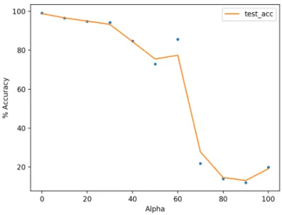
3-1 Adversarial example. The initial image (left) is correctly classified as a panda whereas the perturbed image (right) is classified as a gibbon, even though it looks exactly like the intial one to the human eye [GSS14]. 36 3-2 Test accuracy on true label test points in the uniform label MNIST

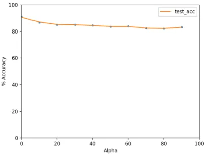
dataset. The generalization error stays relatively low until very high values of alpha (∼ 50), then drops sharply. We attribute the drop to difficulty in optimization rather than a fundamental limitation of the training process. . . 38 3-3 Test accuracy on true label test points in the uniform label CIFAR10

dataset. The generalization accuracy drops slowly but stays relatively high for high noise levels. . . 39 3-4 Test accuracy on true label test points in the uniform label MNIST

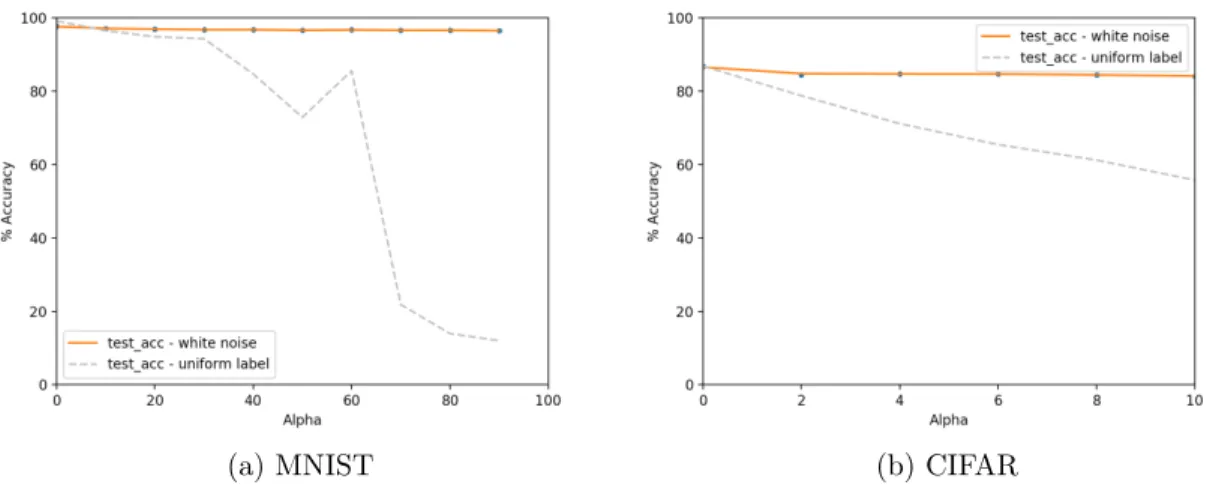
dataset, with a linear model. We can see that the model is very robust to noise and the generalization accuracy is affected minimally. . . 40 3-5 Test accuracy on true label test points in the white noise MNIST and

CIFAR10 datasets. The added noisy images have no effect on the generalization accuracy. The accuracy on the uniform label dataset is added for comparison. . . 42

4-1 Images obtained after adding random gaussian directions to CIFAR10 images. We use different values of 𝜖 from left to right: 0, 50, 500, 5000. We see that for small epsilon the images are modified negligibly. . . . 48

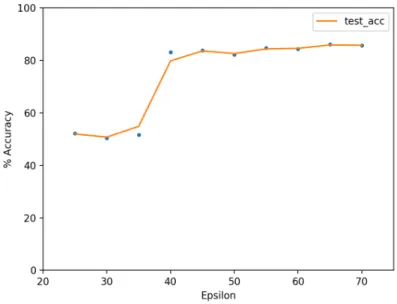
4-2 Test accuracy vs epsilon for the Gaussian Directions dataset with 𝛼 = 9. We see that after 𝜖 = 45 the test accuracy is the same as the accuracy obtained on the CIFAR10 dataset without any augmentation. 49 4-3 Training run on a Gaussian Directions dataset with 𝛼 = 9 and 𝜖 = 45.

The network treats the real and fake images as two distinct entities: it learns on the true dataset first to reach good training set performance, then start memorizing the fake labels. . . 50 4-4 The Gaussian Directions dataset. True training sample (blue) are

sur-rounded by a number of generated data points (red). . . 51 4-5 Training run on a CIFAR0.5 dataset. As in the Gaussian Directions

case, the network learns on the true dataset first. . . 53 4-6 PCA analysis of the activations at the last hidden layer. The top

im-ages show the activations for the entire test dataset, the bottom imim-ages show the activations for real images (x) with their fake counterparts (o). We can clearly see that there’s very little variation along the first 3 PCs for the fake data. The neural network maps the fake data to a very restricted subspace. . . 56 4-7 PCA analysis of the activations at the last hidden layer (single

compo-nent view). The fake inputs activations are significantly concentrated, whereas the real inputs exhibit high variance. . . 57 4-8 The Linear/Quadratic Dataset. The image on the left shows the four

different types of data and the image on the right shows their assigned labels. . . 58 4-9 Train accuracies on the Linear/Quadratic Dataset. The training

accu-racy grows for the L points, which require a simpler classifier, first. . 59

5-1 Train and test accuracies of the comparative run for ReLu and Quad activation. We can see that the linear dataset is easier for ReLU, and the quadratic dataset is easier for Quad. . . 66

5-2 Train and test accuracies of the comparative run for max pool and no max pool networks. The network without max pooling layers achieves high train and test accuracy faster than the network with the pooling layers. . . 68

List of Tables

4.1 Test and train accuracies for Gaussian Directions dataset with different values of 𝛼. We set 𝜖 = 45 for these experiments. We can see that the test accuracy on the real images does not change when we add fake training examples to the dataset. . . 50 4.2 Test accuracies for the probing experiment of the Gaussian Directions

dataset. We can see that the subspace between the true and fake training points is torn between them. However, as we go further than 𝜖-far the network does not recognize 𝑐𝑘 as the label anymore. . . 51

4.3 Test accuracies for CIFAR𝑝. The accuracy goes down linearly with 𝑝:

as more true images get flipped, the true signal vanishes. . . 52 4.4 Train and test accuracies for the real and fake labels dataset. We can

see that after 1 epoch of training the network recognizes what points are on the data manifold. . . 55 5.1 Number of epochs needed to reach 60% train accuracy. The networks

learn significantly faster when training on the data that fits the prior imposed by the activation functions. . . 67

Chapter 1

Introduction

In the past couple of years, deep learning has been the driving force behind successes in many learning and prediction problems. In fact, deep neural networks have allowed unprecedented achievements in fields such as computer vision, natural language pro-cessing, machine translation, games and many others. The systems developed through neural networks achieve, or even surpass, human level performance in these fields. From a practical standpoint, it is therefore apparent that deep neural networks are important, and even essential, for future advances in machine learning.

Nevertheless, we currently have very little understanding of the inner mechanics of deep learning: there is very little theoretical backing for its impressive performance. As any other areas of science, developing simple mathematical rules that underlie the dynamics of deep learning is essential if we want to move forward in the field. Doing so will help with the creation of robust, reliable, and scalable systems. Our work goes along the lines of the science of deep learning. In this thesis, we aim to make a step forward towards understanding the ability of deep neural networks to generalize well. We propose a new perspective on neural networks: they have an inherent inductive bias that pushes them to learn simple things by making them "lazy".

1.1

The Statistical Learning Problem

Machine learning refers to the problem of learning, from a set of observed data, general rules that apply to unseen data. The goal is usually to make predictions or decisions based on these rules. There are three main types of machine learning methods today: supervised learning, unsupervised learning and reinforcement learning. Supervised learning refers to procedures that aim to learn a mapping from inputs 𝑥 to labels 𝑦, whereas unsupervised learning is concerned with learning structure in unlabelled data. The compromise takes the form of reinforcement learning where an agent takes actions in an environment with some reward function and learns with the aim of maximizing the cumulative rewards taken through such actions. In our study, we focus on supervised learning.

1.1.1

Preliminaries and Notation: The Learning Setup

In the supervised learning problem, the goal is to learn a relationship between inputs 𝑥 to outputs 𝑦 from training data. We consider the data distribution 𝒟 on the space 𝒳 × 𝒴 and let 𝑆 = {(𝑥𝑖, 𝑦𝑖) for 𝑖 = 1, ..., 𝑛} denote the training set. The inputs 𝑥𝑖 are

considered to be drawn from the 𝑑−dimensional space R𝑑_{. We focus on the problem}

of classification, where the labels 𝑦𝑖 take a finite number of values from the label set

𝒞. Let ℱ be the space of possible estimators 𝑓 : 𝒳 → 𝒴1 _{and let ℒ : 𝒴 × 𝒴 → [0, ∞)}

be a chosen loss function. The goal of the learning procedure is to find an estimator 𝑓* ∈ ℱ that minimizes the expected risk, or, in other words, the expected error on data drawn from 𝒟:

𝑓* = arg min

𝑓 ∈ℱ

ℰ(𝑓 ), _{where ℰ (𝑓 ) = E}(𝑥,𝑦)∼𝒟[ℒ(𝑓 (𝑥), 𝑦)].

However, as mentioned earlier, we only have access to the training set 𝑆. The

1_{ℱ is not properly defined here. In general, it is considered to be the space of all measurable} functions, but we omit such formality in this case.

procedure thus aims to minimize the empirical risk instead: ˆ 𝑓 = arg min 𝑓 ∈ℱ ˆ ℰ(𝑓 ), where ˆℰ(𝑓 ) = 1 𝑛 𝑛 ∑︁ 𝑖=1 ℒ(𝑓 (𝑥𝑖), 𝑦𝑖).

Minimizing empirical risk assumes that optimizing for the objective ˆℰ is "close enough" to optimizing for the objective ℰ2_{. Additionally, it is in general difficult to}

achieve this without restricting the class of estimators ℱ to some other class ℋ, which is more restricted and has certain desirable properties3_.

1.1.2

Generalization and the Bias-Variance Tradeoff

The goal is to minimize ℰ , yet machine learning procedures minimize ˆℰ. The per-formance of a procedure is thus measured by the closest proxy to the expected risk: the error on a test set, or the generalization error. The latter can be high even if the empirical risk is minimized, a phenomena referred to as overfitting. This is because if the family of estimators ℋ is very large, the number of estimators that can fit the data is also very large, and it is hard for the procedure to pick the one that leads to similar expected and empirical risks. In this case, we say that the procedure has high variance. It is thus common to restrict the family of estimators further to limit the number of estimators that the procedure can find. In doing so, a certain bias away from the data is introduced, and if the family is too small, it will be impossible to fit the training data at all, leading to both training and generalization errors being high. Therefore, there is a tradeoff between bias and variance controlled by the complexity of the family or class of classifiers that are learnable through training, commonly referred to as capacity of the model in inference. However, the bias-variance tradeoff is not solely controlled through capacity. There are other ways to bias the model to learn simple estimators such as adding a regularizing term to the empirical risk objective (known as explicit regularization) or using implicit regularization such as

2_{There are multiple metrics used to define closeness in this context.}

3_{ℋ is usually chosen to be a Reproducible Kernel Hilbert Space because of the desirable properties} of such spaces. These details are not necessary for the development and are thus not explained here.

early stopping.

1.1.3

Feature Maps

In certain machine learning problems such as linear regression, logistic regression and Support Vector Machines (SVM), the family of estimators is taken to be a linear family. However, the mapping between 𝑥 and 𝑦 is often non-linear. Thus, it is common to map the inputs 𝑥 onto a space where their relationship to the labels is linear. Such a transformation is done through feature maps Φ : 𝒳 → ℳ. The feature space ℳ can often have a very high, or even infinite, number of dimensions. Thus, kernel methods are used to avoid having to perform computations using the features Φ(𝑥) [STC04]. Additionally, the choice of the right feature map to use for specific learning problems requires careful feature engineering and is often a difficult problem.

1.2

Deep Learning

Introduced for the first time as the "Neocognitron" [Fuk80], neural networks are currently predominantly used in a wide range of applications. The recent surge of interest in deep learning models came after their exploits in the ImageNet competition in 2012 [KSH12]. Ever since then, they have been applied successfully to a wide range of problems such as image classification, object recognition, speech recognition, control theory, game playing and others [KSH12, HZRS15, GMH13, SHM+16]. The power of deep neural networks comes from the fact that they do not require the practitioners to engineer specific feature maps Φ for the tasks at hand. In fact, through feeding the inputs through a sequence of layers, deep learning models learn a representation of such inputs while learning the input to output mapping.

1.2.1

Preliminaries and Notation

Neural networks are a sequence of layers that consist of a linear transformation fol-lowed by a non-linear activation function. In our work, we will use the following

notation to denote the estimator 𝑓 represented by a depth 𝑘 neural network:

𝑓 : 𝑥 → 𝑊𝑘𝜎𝑘−1(𝑊𝑘−1𝜎𝑘−2(...𝑊2𝜎1(𝑊1𝑥))),

where each 𝑊𝑗 denotes the parameter matrix at layer 𝑗 and each 𝜎𝑗 denotes the

activation function at layer 𝑗4. In our treatment, we mainly consider the ReLU activation function 𝑥 → max{𝑥, 0}. Additionally, the height ℎ of the network is usually defined as the largest row or column dimension of the matrices 𝑊1, ...𝑊𝑘.

From a statistical learning perspective, the parameters of the network (essentially the entries of the matrices) serve as an index into the space of estimators. Therefore, in deep learning, minimizing the empirical risk corresponds to learning the parameters of the network that lead to the best estimator. We denote all the parameters of the network by the vector 𝜃5_{. Thus, the network is the estimator 𝑓}

𝜃 parametrized by

𝜃. The class of estimators that can be represented by the network is defined by its architecture, which englobes choices such as the depth of the network, the type of the different layers (convolutional, fully connected, max pool etc.), and the height of these layers.

Let ℒ be an arbitrary loss function (it is usually the cross-entropy loss for classi-fication problems). The most commonly used method to learn the parameters 𝜃 that minimize the empirical loss is Gradient Descent (GD). GD is an iterative first-order method that moves the network parameters in the direction opposite to the gradient, or equivalently, the direction of steepest descent with respect to the objective. The update step in GD at time 𝑡 is:

𝜃𝑡+1 ← 𝜃𝑡_{− 𝜂} 𝜕 𝜕𝜃𝑡 𝑛 ∑︁ 𝑖=1 ℒ(𝑓𝜃𝑡(𝑥_𝑖), 𝑦_𝑖),

where 𝜂 is a hyperparameter referred to as the learning rate. In practice, GD is usually replaced by its variant, Stochastic Gradient Descent (SGD). Instead of summing over all the training examples at each step (which can be very computationally intensive),

4_{The activations functions 𝜎 are required to be Lipchitz continuous in general.} 5_{𝜃 corresponds to stacking the parameters of the matrices 𝑊}

SGD approximates the empirical loss by sampling one training point (𝑥𝑖, 𝑦𝑖) (or a

batch of training points) at a time and computing the loss on the point for the update. The update is as follows:

𝜃𝑡+1 ← 𝜃𝑡_{− 𝜂} 𝜕

𝜕𝜃𝑡ℒ(𝑓𝜃𝑡(𝑥𝑖), 𝑦𝑖).

Practically, the computation of the gradients is done via backpropagation [LBH15]. Additionally, many variants of SGD are used for different types of networks in practice such as adaptive methods that adapt the learning rate dynamically like AdaDelta [Zei12] and Adam [KB14], or second-order methods that use additional information about the Hessian like K-FAC [MG15].

1.2.2

The Science of Deep Learning

In the past couple of years, deep neural networks have proven to be extremely powerful methods from a practical point of view. However, there is very little theory around deep learning. The root of this shortcoming comes from the fact that most of the developments in learning theory are for problems that fall under the umbrella of estimators that are linear in the input data 𝑥 or the features Φ(𝑥), and that are chosen to have "nice" properties6_{. The estimators represented in deep networks are}

not linear and do not have such "nice" properties. To circumvent this, a line of research focuses on studying "shallow" networks, which are simplified versions of the architectures used in practice, to develop theoretical guarantees around such manageable setups. Another line of research focuses on explaining the behavior of deep neural networks through a mix of empirical and theoretical analyses. These works are mainly concerned with developing a science around deep learning. As for any novel phenomena, the science is still in early stages and the theoretical evidence is usually limited in scope and requires relatively strong assumptions. The goal is to develop a unified understanding of the mechanics of deep learning both from an optimization and generalization perspective. Our work follows this line of thought

and focuses on the generalization performance of deep neural networks.

1.2.3

Generalization in Deep Learning

The most commonly used neural network architectures are heavily overparametrized [ZBH+_{16]: the number of parameters is often larger than the number of samples used}

for training. Therefore, the class of estimators represented by the neural networks is highly complex. In fact, such networks can represent any function given enough overparametrization: they are universal approximators [HSW89]. As explained in 1.1.2, traditional learning theory suggests that such networks should have a hard time generalizing. However, this is not the case in practice: often, increasing the number of parameters leads to an increase in test set accuracy [LSS14]. In our work, we investigate this odd behavior of deep learning models and tie it to a notion of inductive bias inherent to the networks.

1.3

Contributions: the Inductive Bias

The ultimate goal of any statistical learning system is to generalize, or in other words, perform well on unseen data. To do so, the training procedure needs to avoid overfit-ting: the models needs to use a relatively small number of instances to learn simple rules that apply to a large number of instances. Therefore, the goal is for the learning process to be as similar as possible to induction. Traditionally, learning procedures are coupled with various methods that push them to induce such as model complexity restriction, regularization and early stopping. In our work, we propose evidence that neural networks have an inherent bias to induce: the inductive bias.

1.3.1

The Inductive Bias: a Definition

Induction is defined as the "inference of a general law from particular instances" [Oxf18]. The aim of most scientific fields is to induce. In fact, scientists often explain observed practical phenomena via compact rules that summarize the underlying

dy-namics of the observations. Newton could have written a large table mapping each observed initial condition to trajectories of moving objects, but he came up with sim-ple equations that summarize the behavior of such objects instead. Our works sug-gests that deep learning models have an affinity to induce. They prioritize learning simple hypotheses from noisy observations instead of memorizing said observations.

1.3.2

Laziness, or Learning Simple Things First

As intellectual pleasing as it might be, the idea that the inductive bias in neural networks comes from a certain "human" drive to learn general dynamics is obviously far from being true. Our results show that the root of the inductive bias is a certain laziness of deep learning models: they tend to learn on simple structured data first even if they have enough capacity to learn on the more complicated unstructured data. We propose a proof of concept that demonstrates that deep networks prioritize learning simple classification boundaries before complex and elaborate boundaries and tie this phenomena to the generalization ability of the networks.

1.3.3

Simplicity is Not General

In general, there is no global ordering for simplicity. Some boundaries may be con-sidered simple for some networks and complex for others. We propose evidence that simplicity is defined by the implicit priors inherent to deep learning procedures. In this respect, we call for careful reasoning about the a priori beliefs that deep net-works incorporate as they can heavily bias the training procedure and impact the performance from both optimization and generalization standpoints.

1.4

Outline

The thesis is organized as follows. Chapter 2 synthesizes the key findings in the works related to the topic. In chapter 3, we discuss the robustness of deep learning models to large amounts of noise and tie it to their laziness. The latter is discussed

extensively in chapter 4, where we propose evidence showing the inductive bias at play in deep learning procedures. In the chapter, we also present empirical results that suggest that neural networks learn simple things first and propose the phenomena as a potential root of the bias to induce. Additionally, we redefine the concept of simplicity in chapter 5 as the byproduct of the a piori conditioning of the networks. Chapter 6 summarizes our results and proposes potential avenues for future research.

Chapter 2

Related Works

Deep learning models have recently helped achieve a large number of successes in many fields such as image classification, machine translation and others. However, there is still very little theory around such models and how they work. In fact, the current machine learning toolkit is insufficient to explain the performance of neural networks from both optimization and generalization standpoints. Understanding deep learning models’ ability to generalize is thus a very active area of research in machine learning and statistics today.

2.1

The Quest to Uncover Deep Learning

General-ization

The traditional machine learning view on generalization is that models with high ca-pacity, or number of parameters larger than the number of samples, tend to exhibit very poor test set performance [GBC16]. This is because such models have the abil-ity to memorize and thus overfit the training set. However, although often severely overparametrized, deep neural networks have exhibited a phenomenal ability to gener-alize well on unseen data. There is very little theoretical backing for this phenomena. In fact, deep neural networks are considered to be universal approximators: given enough layer width, they are capable of approximating any measurable function to

any desired degree of accuracy [HSW89]. The traditional learning theory paradigm thus tells us that such networks should in principle heavily overfit the training set and struggle with achieving high generalization accuracy. The current theory is thus clearly inapplicable in this situation and there is a range of investigative works that aim to unveil the roots of generalization in deep learning.

2.1.1

Stochastic Gradient Descent (SGD) as a Driver of

Gen-eralization

The ability of neural networks to generalize has been linked to the driving force behind their optimization: stochastic gradient descent. In [ZLR+_{18], it is claimed that SGD}

optimization pushes the network parameters towards "flat minima" instead of "sharp minima". This is because such minima make the solutions more robust to the inherent fluctuations between train and test sets. SGD help achieve such minima because of the inherent noise in the gradients computed by the method. Similar results are found in [KMN+16], where they argue that larger batch sizes lead to "sharp "minima", and hurt the generalization performance, since larger batch sizes lead to a reduced stochasticity in the gradient updates. We follow a different path in our work and focus on the inherent biases in the models rather than properties of the optimization procedures.

2.1.2

Overparametrization as a Feature

Another line of works studies the relationship between overparametrization and gen-eralization in deep neural networks. Although overparametrization is traditionally considered an inhibitor of generalization, there is evidence suggesting that they do not hold such a function in deep learning. Such evidence shows that increasing the number of parameters can often lead to better generalization accuracy because the additional parameters make training faster and the optimization problem eas-ier [LSS14, AGNZ18]. The work in [LL18] couples the effects of SGD and over-parametrization. They prove that sufficient overparametrization leads SGD to learn

parameters that are close to the random initialization. The idea of the model pa-rameters moving little in terms of common distance metrics is linked to good gen-eralization error since moving little is considered a form of implicit regularization in learning theory. This idea is investigated in a variety of other works. The works [NLB+18a] propose a capacity bound base on the Frobenius (L2) distance between the

parameters at convergence and the randomly initialized parameters that is correlated with the test error. Such a distance is also argued to decrease with overparametriza-tion. Additionally, assumptions on the same distance metric are used in [ALL18] to prove that the generalization error of the solution can be independent of the number of parameters; an idea also investigated in [GRS17]. These works propose evidence towards some sort of inductive bias inherent to the networks that stems from the coupling of overparametrization, SGD and random initialization. Our results extend the investigation of concept.

2.1.3

Interpolation is not Equivalent to Overfitting

Traditional statistical learning theory does not explain the empirical performance of deep learning. In fact, the bias-variance tradeoff is central to the understanding of generalization for traditional learning methods such as kernel regression and support vector machines (SVM) [SSBD14, CST00]. Many measures of complexity such as VC-dimension and regularization mechanisms have been developed to address the tradeoff. However, such mechanisms fail to capture the behavior of deep neural networks [ZBH+16]. In fact, such analyses allow learning procedures to fit the data perfectly only when there is very little noise in the sampling process that leads to the empirical set, which is usually not the case for the applications in question. Thus, statistical learning is currently witnessing a surge of works that rethink the bias variance tradeoff with the aim to reconcile learning theory with the performance of methods such as kernel machines, boosting, random forests, and deep learning.

The bias variance tradeoff suggests that fitting the data perfectly, or interpolating it, is equivalent to overfitting. However, some recent works show that this equiva-lence is not general. The works in [LR18] propose a proof of concept rejecting this

equivalence. They study the Kernel Regression method with a very high dimensional Hilbert space ℋ. In general, such a method has the ability to fit the training set perfectly and a regularization term 𝜆||𝑓 ||2_ℋ (where 𝑓 is an estimator chosen from the family ℋ) is usually added to the objective function to avoid overfitting. The parameter 𝜆, which is used to balance bias-variance tradeoff, is usually set to 0 in practice. To explain this, they propose Kernel "Ridgeless" Regression and show that minimum-norm interpolated solution can have mechanisms of implicit regularization that find their root in high dimensionality, the curvature of the kernel function and favorable data geometry, and that are isolated from the bias-variance tradeoff. These results are reinforced in [BRT18] where it is proved that interpolation in the context of non-parametric regression and square loss prediction can lead to optimal rates. This is because, although the interpolating estimator fits all training points, the influence of each point is "local" and the estimator is, in aggregate, pulled towards the optimal estimator. The works also show a coexistence between bias-variance tradeoff and in-terpolation in the estimators studied. The generalization properties of inin-terpolation schemes are also studied in [BHM18]. The performance of interpolation is analyzed through the lens of local classification methods such as geometric simplical interpo-lation and nearest neighbor rule based schemes. A running hypothesis is that this new paradigm in learning theory explains the out of sample performance of neural networks. Our work proposes evidence towards this hypothesis.

2.2

Memorization in Deep Learning

Deep neural networks generalize well but they have the capacity to memorize input to output mappings. One potential hypothesis suggests that stochastic gradient descent based training methods coupled with early stopping are enough to prevent the neural networks to memorize during the training procedure. However, empirical evidence suggests that this is not the case and that deep neural networks can overfit and mem-orize random noise. The experiments in [ZBH+_{16] demonstrate that neural networks,}

Therefore, it does not seem that the lack of ability to memorize noise is what prevents neural networks from overfitting that noise.

2.2.1

Noise Robustness in Deep Learning

Deep learning methods have exhibited large robustness to noise, even if they can fit the noise. The work in [RVBS17] suggests that deep networks exhibit extreme ro-bustness to noise in the label space. The experiments they ran consists of augmenting datasets such as MNIST and CIFAR10 with an large number of randomly (uniformly or with bias) labeled images drawn from the datasets. The results show that the gen-eralization performance is relatively hurt very little, even when noisy training points severely outnumber the signal bearing points, as long as there is enough points from the latter type. We extend these results and analyze them in the context of the inductive bias and laziness of neural networks.

2.2.2

Memorization is Secondary

The neural network architectures used in practice can deal with a large amount of noise. In fact, they treat noisy and real data differently, as suggested in [AJB+_17].

The work mentioned proposes a practical definition of memorization as training on noise, as well as a way to measure hardness of the hypotheses learned by the networks through the proposed Critical Sampling Ratio. They suggest that neural networks do not memorize real data, but only memorize noise. Additionally, they proposal empirical evidence that suggests that neural networks learn on simple patterns first and memorize noise second, and that the networks take advantage of shared patterns and structure between training examples to differentiate between the two types of data. They also link higher capacity to the ability to generalize better in high noise setups, since network use the extra capacity to memorize.

The idea that neural networks have an inherent bias to learn simple hypotheses is also discussed in [NTS14]. They propose empirical and theoretical evidence that a type of implicit regularization, orthogonal to capacity control, plays a big role in the

generalization of deep neural networks. They coin it the "Real Inductive Bias". They draw an analogy to random matrix theory to suggest implicit norm regularization as a potential source for the inductive bias. The result they present is that such implicit capacity control takes the form of L1 regularization in the top layer for infinite

two-layer networks with L2 weight decay. We center our analyses around the proposed

inductive bias hypothesis and propose evidence to back it.

2.3

Priors in Deep Learning

The idea that neural networks generalize because they do not move much has lead to extensive research around the initial configuration of such models. Such configurations take the form of priors ingrained in the model. Although priors are more commonly used in fully probabilistic settings, some works in the Bayesian literature propose a broader definition of priors as a summary of beliefs before the model is run. In some instances, such beliefs can in fact be influenced by the likelihood or the model itself [GSB17]. Armed with this perspective, there is a range of works that investigate priors in deep learning.

2.3.1

Priors as Network Biases

Priors are considered to heavily influence the training procedure of deep architec-tures. In fact, convolutional neural networks (CNNs) were introduced in [LBBH98] as a superior method for image classification because of the priors they hold such as translation independence. Following the same line of thought, the work in [UVL17] presents evidence that the structures of ConvNets hold a large number of image statis-tics a priori. They use non-trained ConvNets for inverse problems such as denoising and show that the structures with randomly initialized parameters are sufficient for good performance. On the flip side, some works suggest that bad priors can degrade performance significantly. In [LLM+18], ConvNets are shown to perform very poorly on tasks that involve translation dependence. The work also proposes a new network, called CoordConv, that holds better priors for such tasks. The importance of priors

has led recent works to focus on the development of priors that fit different tasks or even different learning paradigms. A "consciousness" prior is proposed in [Ben17] as a mechanism to bias the network towards learning representations in the abstract space rather than the pixel space. In our work, we propose a broad study of different types of deep learning priors and analyze their effect in the context of the inductive bias.

Chapter 3

On the Noise Robustness of Deep

Learning Models

3.1

Introdution

In this section, we will study Deep Learning models’ robustness to what we refer to as "benign" noise. In general, deep neural networks tend to exhibit superior robust-ness to noise when compared to other machine learning methods such as SVMs or kernel regression. In this context, robustness refers to consistency in terms of gener-alization performance: robust models are models for which the prediction accuracy is unchanged or changed negligibly when trained on a dataset with high noise levels. Our results confirm that the test accuracy is changed very little even when the deep learning models are simple and there is a significant amount of noise. Through these results, we also make this statement about robustness to noise more precise and tie it to a more fundamental property of deep neural networks: "laziness" (which will be discussed extensively in chapter 4).

3.1.1

Benign Noise and Adverserial Noise

We use the term benign noise to refer to noise, which could be on the input space or the label space, that is the result of a purely stochastic process and that is not crafted

Figure 3-1: Adversarial example. The initial image (left) is correctly classified as a panda whereas the perturbed image (right) is classified as a gibbon, even though it looks exactly like the intial one to the human eye [GSS14].

for the purpose of fooling the network or hurting its performance. We carefully define the concept to distinguish this type of noise from adversarial noise that is usually used in adversarial attacks. Malicious noise corresponds to noise that is carefully crafted to fool the learning algorithm without changing the input in the eyes of a human observer [DDM+04] . This type of noise has also been studied extensively in the context of deep learning for image classification [SZS+_{13, BCM}+_{17]. Figure 3-1}

is an instance of a typical adversarial example. These examples are usually created through solving the optimization problem that is based on each test points (𝑥𝑖, 𝑦𝑖):

𝑥′_𝑖 = arg max

𝛿

ℒ(𝜃, 𝑥𝑖+ 𝛿, 𝑦𝑖).

Solving this optimization problem and coming up with defenses against the algorithms that solve it is a very active area of research in the field [MMS+17]. In our study, we are not concerned with the impact of test set noise on the predictions emitted by the neural networks: we focus on the impact of training set noise. We study both label and image space noise that is generated randomly, without malicious intent. This is an interesting type of noise to study if we operate under the assumption that the noise is better modeled by some stochastic process rather than by the result of an adversarial procedure; an assumption that holds in a variety of "real world" settings. To this extent, we replicate and extend results from [RVBS17]. Our findings agree

with the results of the paper: the experiments we ran and our analysis of the results point towards robustness to heavy input and output space noise in deep learning models. From a generalization perspective, the models are unchanged. However, sig-nificant levels of noise can impact the optimization procedure, which makes robustness to noise require fine model tuning.

3.2

Generalization with High Output Domain Noise

In this section, we extend some of the work in [RVBS17] to further the understanding of deep learning’s performance in setups with low signal to noise ratio. More specifi-cally, we study situations where the number of "true" images that contribute to the signal we aim to learn is significantly outnumbered by the number of "fake" images that have no, or even negative, contribution to the signal of interest. The behavior is studied on an image classification setup, where for each truly labelled image we add a number of randomly drawn labels. More formally, let the number of training examples be 𝑛. For each training example (𝑥𝑖, 𝑦𝑖), we generate 𝛼 training samples

such that each generated "fake" sample (𝑥𝑓_𝑖, 𝑦_𝑖𝑓) follows (where 𝒰 denotes the uniform distribution and 𝒞 denotes the set of possible classes in the image classification setup):

𝑥𝑓_𝑖 = 𝑥𝑖

𝑦_𝑖𝑓 ∼ 𝒰 [𝒞].

We calls refer to this dataset as the "uniform label" dataset. Note that in this case, we do not modify the original training dataset but merely augment it.

3.2.1

Non Linear Networks

We first investigate the behavior of network with non-linear activations (ReLU more specifically). Figure 3-2 outlines the result of runs with different values of 𝛼 on MNIST [LC10]. In this experiment, we use a simple 4-layer convolutional neural network, with an SGD optimizer run for 100 epochs. It is clear that even without

Figure 3-2: Test accuracy on true label test points in the uniform label MNIST dataset. The generalization error stays relatively low until very high values of alpha (∼ 50), then drops sharply. We attribute the drop to difficulty in optimization rather than a fundamental limitation of the training process.

excessive tuning, when compared to the state-of-the-art architectures, the network’s generalization performance is not significantly hurt until a very high value of 𝛼, around 50 more specifically. After 𝛼 = 50, we observe a degradation of the test accuracy. This seems to be the consequence of the optimization becoming more difficult which calls for additional hyper-parameter tuning to enhance the optimization procedure. We used a standard, AlexNet based [KSH12], 4-layer architecture and intentionally stayed away from very specific tuning to make sure that the results proposed are a property of a wide class of neural networks and not a specific configuration of the run. We used standard Stochastic Gradient descent for optimization. Overall, the results point towards robustness to massive label noise, since when 𝛼 = 50, there are 50 randomly labelled images for each image with a true label, thus, the network is exhibiting good generalization performance in an extremely high noise-to-signal ratio environment.

Additionally, we ran the same experiment on CIFAR10 [KNH]. The model we used for CIFAR10 is also standard: a 6-layer ConvNet optimized via momentum

Figure 3-3: Test accuracy on true label test points in the uniform label CIFAR10 dataset. The generalization accuracy drops slowly but stays relatively high for high noise levels.

SGD. We observe similar trends to what we observed with MNIST, but we do so in lower noise-to-signal ratio domains (Figure 3-3): after 𝛼 = 10, the generalization accuracy gets hurt and drops relatively sharply.

3.2.2

Linear Networks

To investigate the hypothesis further, we look into the behavior of linear networks when faced with high label noise. We run the experiment on MNIST with the same ar-chitecture, except that we drop the non-linear activation functions, specifically ReLU. The results presented in Figure 3-4 show that linear models are even more robust. The drop in accuracy observed for high 𝛼 when the network used ReLU activation is not observed anymore. In general, deep linear networks are "easier" to optimize than their non-linear counterparts. Additionally, the linear model has the same number of parameters as the ReLU based model, so there is no capacity difference between them. Therefore, the result reinforces our hypothesis: the drop in accuracy for the non-linear networks arises because of a difficulty in the optimization domain and not the generalization domain.

Figure 3-4: Test accuracy on true label test points in the uniform label MNIST dataset, with a linear model. We can see that the model is very robust to noise and the generalization accuracy is affected minimally.

Our investigation shows that deep learning models are robust to excessive amount of label noise: the network’s learning procedure is unfazed even when 99% of the training dataset is corrupted. It is apparent that the network use a "majority" deci-sion rule during training, thus, as long as the true label is marginally overrepresented in the relevant space, the network will pick it as the correct label for the sub-space. More broadly, this behavior is hinting at an interesting and more general behavior: deep networks have a predisposition to assign one label to the sub-space in question instead of "overfitting" and memorizing the uniform labels. In other words, the networks are conditioned to learn simple decision rules.

In this section, we analyzed robustness to label noise, but noise can also manifest itself in the input domain. We will analyze this next.

3.3

Generalization with High Input and Output

Do-mains Noise

In the previous section, we studied noise on the label space, so the inputs were un-changed. We now generate new training points by adding gaussian noise to the input images; let the input images 𝑥𝑖 lie in R𝑑, let 𝒩 denote the multivariate normal

distri-bution, let 0𝑑, 𝐼𝑑, denote the 𝑑-dimensional 0 vector and identity matrix respectively,

and let 𝜎2 denote variance, each fake training point (𝑥𝑓_𝑖, 𝑦_𝑖𝑓) is generated as: 𝛾 ∼ 𝒩 (0𝑑, 𝜎2𝐼𝑑)

𝑥𝑓_𝑖 = 𝑥𝑖+ 𝛾

𝑦_𝑖𝑓 ∼ 𝒰 [𝒞].

We refer to this dataset as the "white noise" dataset.

3.3.1

Input Domain Noise as an "Easier" Task

The white noise dataset can help us investigate how the neural network assigns labels to sub-spaces. We use the same models as in Section 3.2 to train on augmented datasets generated from MNIST and CIFAR10. The results are presented in Figure 3-5. The generalization accuracy is effectively completely oblivious to the addition of noisy images in the dataset: it is the same across a wide range of alphas for both datasets. In some way, this shows that the white noise dataset is a strictly "harder" task than training on the uniform label.

3.3.2

Towards the "Laziness" Property of Deep Neural

Net-works

For the MNIST dataset, a simple argument could be made about the results: the white noise affects the usually empty areas of the images and can create a simple "backdoor" for classification. However, in the more general case (CIFAR10 for example), this

(a) MNIST (b) CIFAR

Figure 3-5: Test accuracy on true label test points in the white noise MNIST and CIFAR10 datasets. The added noisy images have no effect on the generalization accuracy. The accuracy on the uniform label dataset is added for comparison.

is not necessarily obvious a priori: as discussed earlier, the network can be using a majority decision rule when he sees different signals that correspond to the same image; that does not necessarily entail that the network would learn the same decision rule when it sees neighboring images with different labels.

The reasoning used above does not seem to be sufficient to explain what is going on in this situation. The fact that the accuracy is untouched shows that the additional training examples do not influence the training process and they are somewhat ignored by the network. This ties back to the hypothesis we proposed earlier about networks aiming to learn simple things first. In fact, the additional training points are very proximal points, in terms of many distance metrics such as 𝐿2 (Frobenius) or 𝐿∞

norm, and they have different labels, they are thus not "simple" in the sense that sophisticated decision boundaries would be required to classify them correctly. The network does not get influenced by these data points and prioritizes the "real" data points that exhibit more structure. In order to do this, the networks need to be preconditioned to learn simple things first, or in other words, the network have to have an implicit inductive bias. We will discuss this extensively in chapter 4.

Additionally, the ability of the network to disregard the noisy training examples is interesting in and of itself. The generated points can be understood as being outside

the data manifold and the network seems to be aware of that. We will make this statement more precise in the next chapter.

Chapter 4

Learning Simple Things First: On the

Inductive Bias in Deep Learning

Models

In the last chapter, we observed an interesting property of deep neural networks: they can handle a massive amount of noise, both in label and images spaces. Such a property points towards the networks being able to ignore fake noisy inputs and focus on the true signal bearing inputs. In this chapter, we will analyze the cause of this behavior: deep learning models prefer to learn the simple things, and noisy inputs are not simple.

4.1

Introduction

Our work aims to provide evidence towards deep learning models having an inherent inductive bias: they tend to learn underlying rules, in other words, simple models, instead of memorizing specific training examples. If our hypothesis is true, this would explain the relatively good generalization performance typically observed in deep learning procedures. Such a behavior is surprising for deep models since they are usually highly over-parametrized, and we would thus expect the traditional statistical learning theory bias-variance tradeoff to cause a high generalization gap. In our study,

we tie our results to an active area of research in statistical learning theory that rejects the traditional bias variance tradeoff: recent works in the literature propose evidence that fitting does not imply overfitting and models’ bias-variance tradeoffs are not necessarily tied to the training set performance[BRT18, LR18, BHM18]. The procedures in question learn simple decision rules, even if they interpolate the data. The hypothesis of inductive bias would be a step forward towards reconciling deep learning’s performance whith this new thread in learning theory.

As discussed in Chapter 2, the idea of inductive bias in deep learning is not novel. It has been hypothesized that deep learning models have such a bias, which manifests itself in the form of implicit regularization [NTS14]. This regularization mechanism is independent of capacity control. We aim at making this statement more precise and study the mechanism through which deep learning models are biased to learn simple and general decision rules.

The results of Chapter 3 show that even if there is a significant amount of noise, neural networks still generalize well. As mentioned earlier, this could imply that the models are pre-conditioned to learn simple rules: noisy inputs are more complex than true inputs since they have significantly less structure. We extend this result in section 4.2, which unveils a very interesting property of the networks: they learn as if fake data is not there. Our results are augmented by some additional experiments in section 4.3 that show that the networks are "aware" of the type of data they are learning from: noisy fake data or true structured data. We tie this behavior of neural networks to their aim at working with compressed representations of the problem. In section 4.4, we create a synthetic experimental setup where we train simple networks on data with varying degrees of simplicity to show that the networks learn simple things first. Such a behavior would explain the affinity of deep learning models to compress the space in which they are operating.

4.2

A Surprising Behavior: Generalization is

Obliv-ious to Fake Images When it Matters

In this section, we study the generalization of deep neural networks when faced with a mix of "true" structured data and "fake" unstructured data. Our results show that the generalization error is unaffected by the addition of the unstructured data: mem-orization of the fake data happens after learning the underlying principles governing the real data, and when it does happen, it does not impact "real learning".

4.2.1

Data Generation: the Gaussian Directions and CIFAR

The datasets used for the experiments are divided into two parts: true and fake. The true dataset contains image and label pairs drawn from CIFAR10. The fake dataset is synthetically generated based on the CIFAR10 images. We use ˆ𝐷 and

ˆ

𝐷𝑓 _{to denote the true and fake datasets respectively. There are two types of fake}

datasets used in this section. In section 4.2.3, the fake dataset contains the real images with randomly assigned labels. In this case, a fraction of the training examples from CIFAR10 are randomly assigned a uniform label. We use the parameter 𝑝 to denote the probability of changing an image’s label to a uniform label, thus, the overall dataset contains 𝑛 = 50, 000 training points, with a fraction ∼ 𝑝 of them having uniform labels instead of their true label. We call such datasets CIFAR𝑝. In section

4.2.2, the fake dataset is not generated from editing CIFAR10; it is compromised of 𝑛𝛼 generated training points: for each image-label pair (𝑥𝑖, 𝑦𝑖) in the CIFAR10

dataset, create 𝛼 fake training points (𝑥𝑓_𝑖, 𝑥𝑓_𝑖) as, where 𝑑 denotes the dimension of the images, and 𝜖 a real values parameter:

𝛾 ∼ 𝒩 (0𝑑, 𝐼𝑑)

𝑥𝑓_𝑖 = 𝑥𝑖+ 𝜖

𝛾 ||𝛾||2

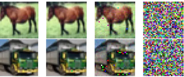
Figure 4-1: Images obtained after adding random gaussian directions to CIFAR10 images. We use different values of 𝜖 from left to right: 0, 50, 500, 5000. We see that for small epsilon the images are modified negligibly.

Essentially, the fake points corresponding to each true point, are composed of images dispersed randomly over the 𝜖 hyper-sphere and uniform labels that are misleading (not the true label). We will call this dataset the "Gaussian directions" dataset. Figure 4-1 shows some true images with their fake counterparts for different values of 𝜖. In general, 𝜖 needs to be on the order of 103 for the images to be modified significantly. This makes sense since a norm of 𝜖 ∼ 103 _{in 𝑑 = 3, 072 dimensional}

space, corresponds to an average shift on the order of 1 pixel.

4.2.2

Generalization with Gaussian Directions

We ran a 6-layer ConvNet on Gaussian Directions datasets with different values of 𝛼 and 𝜖. Figure 4-2 shows the generalization accuracy for different values of 𝜖. The poor performance for the low values of the gaussian norm is explained by the fact that the images stay essentially the same (the noise is imperceptible) as we discussed in section 4.2.1. This is an interesting property since it seems that if the fake images are far "enough" from the true images, the training on the true images does not get perturbed, even if the fraction 𝛼 of fake points to true points is very high. We have also run the experiment for different values of 𝛼. The results are shown in table 4.1. There is no dependence on 𝛼 when 𝜖 is high enough: even when the fraction of true

Figure 4-2: Test accuracy vs epsilon for the Gaussian Directions dataset with 𝛼 = 9. We see that after 𝜖 = 45 the test accuracy is the same as the accuracy obtained on the CIFAR10 dataset without any augmentation.

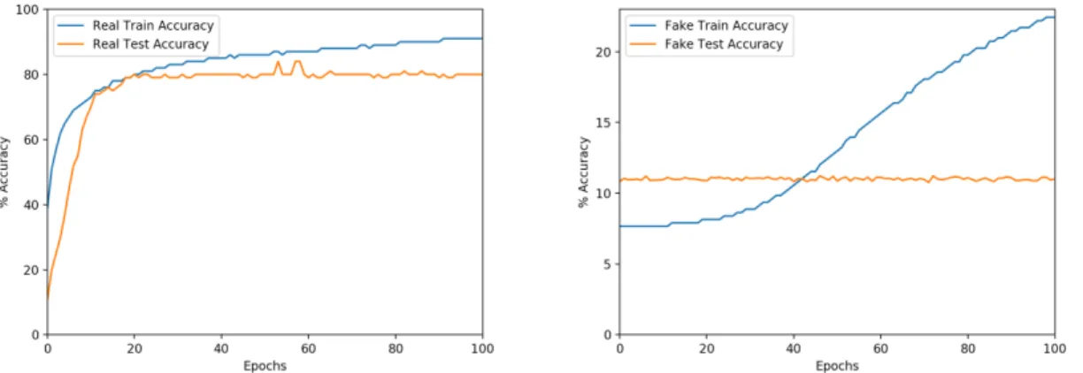
input points to fake inputs is as low as 5%, the network’s generalization performance is unchanged. Additionally, we can see that the fake data gets memorized to some extent, since the train accuracy is above chance (> 10%); this means that even though the network memorizes noise the memorization does not impact the test accuracy or the network’s learning on the true structured data. This idea has been observed in [AJB+_17].

Additionally, the network seems to deal with true and fake images differently. If we look at any of the runs mentioned previously (an example is in Figure 4-3), we see that the training accuracy progresses faster and earlier for the true dataset. In other words, the network trains on the true dataset first, ignoring the fake images, until it reaches good accuracy and converges. The training on the fake images does not start till after the training on the true images is over, and it corresponds to memorizing the fake, unstructured labels: the test accuracy is fixed around random. It is clear from this experiment that the network prioritizes learning the true labels.

This behavior of neural networks is interesting. To see this, we reason about the Gaussian Directions dataset. We denote by ˆ𝐷𝑐𝑘 the subset of the true training set

𝛼 Total Train Accuracy Real Train Accuracy Fake Train Accuracy

9 28.43% 95.40% 21.32%

19 27.81% 96.12% 24.37%

29 26.78% 95.32% 24.52%

𝛼 Total Test Accuracy Real Test Accuracy Fake Test Accuracy

9 46.71% 83.42% 10.00%

19 47.27% 84.54% 10.00%

29 46.07% 82.13% 10.00%

Table 4.1: Test and train accuracies for Gaussian Directions dataset with different values of 𝛼. We set 𝜖 = 45 for these experiments. We can see that the test accuracy on the real images does not change when we add fake training examples to the dataset.

Figure 4-3: Training run on a Gaussian Directions dataset with 𝛼 = 9 and 𝜖 = 45. The network treats the real and fake images as two distinct entities: it learns on the true dataset first to reach good training set performance, then start memorizing the fake labels.

that pertains to class 𝑐𝑘∈ 𝒞, ˆ𝐷𝑐𝑘 = {∀(𝑥, 𝑦) ∈ ˆ𝐷 𝑠.𝑡 𝑦 = 𝑐𝑘}. We also denote by ˆ𝐷

𝑓 𝑐𝑘

the fake training points that pertain to class 𝑐𝑘: ˆ𝐷𝑓𝑐𝑘 = {∀(𝑥

𝑓_{, 𝑦}𝑓_{) ∈ ˆ𝐷}𝑓 _{𝑠.𝑡 𝑦}𝑓 _{= 𝑐} 𝑘}.

Lets look at one point (𝑥𝑖, 𝑦𝑖) ∈ ˆ𝐷𝑐𝑘 and one of its 𝛼 fake counter parts (𝑥

𝑓 𝑖, 𝑦

𝑓

𝑖) ∈ ˆ𝐷𝑐𝑓𝑘.

As discussed previously, the L2 distance between these two points is ||𝑥𝑖− 𝑥𝑓𝑖||22 = 𝜖.

Let the distance between 𝑥𝑖 and some arbitrary test point 𝑥′𝑖 that belong to class 𝑐𝑘

be denoted as 𝛿. In our experimental setup, we have 𝜖 << 𝛿 (as can also be seen in Figure 4-1). In some sense, the fake training points fall "between" the true training points and the true test points. Figure 4-4 proposes a pictorial representation of the dataset. Thus, it would be reasonable to expect these fake training points to act as

Figure 4-4: The Gaussian Directions dataset. True training sample (blue) are sur-rounded by a number of generated data points (red).

some form of "barrier" that can modify the class label for images that are further away from 𝑥𝑖. The results of our experiments show that such a barrier does not exist,

as the label is still 𝑐𝑘 when we go further out, and reach test points. However, there

is some sort of barrier that gets created. We used the models trained on the Gaussian direction dataset with certain 𝛼 and 𝜖 and probed the landscape, or more specifically the subspace to label map. To do that, we generate new test points with images generated through the same procedure as for the fake training set but with distance a fraction of 𝜖 and labels 𝑐𝑘. The results are summarized in table 4.2. The test accuracy

is affected when we go further away from the training points. The label is modified and influenced when we move along a random direction, so the barrier exists along most random directions. Nevertheless, it does not exist when we move within a very specific subspace, which contains the true test points and other true training points: the data manifold. This is evidence that the network is aware of the manifold. We will discuss this further in section 4.3.

distance Test Accuracy

0.1𝜖 82.53%

0.5𝜖 72.45%

1.5𝜖 2.00%

2.0𝜖 2.00%

Table 4.2: Test accuracies for the probing experiment of the Gaussian Directions dataset. We can see that the subspace between the true and fake training points is torn between them. However, as we go further than 𝜖-far the network does not recognize 𝑐𝑘 as the label anymore.

4.2.3

Generalization in CIFAR

In this section, we provide additional evidence towards our claim, before we dig deeper into the data manifold. We run experiments on the CIFAR𝑝 dataset described

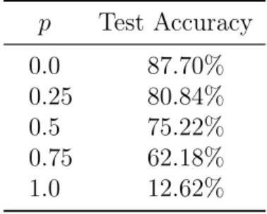
in section 4.2.1 with different values of the proportion 𝑝. The results reported in table 4.3 show that the accuracy drops linearly with 𝑝. Therefore, the network’s learning procedure is impacted in this case. This seems to contradict the results of section 4.2.2 a priori. However, in this case, we edited the dataset and not augmented it. Thus, there are less training points in general, and the drop in accuracy comes mainly from a sample complexity argument. In fact, we still observe the behavior of the networks on the Gaussian Directions: it learns from the true data first (Figure 4-5). Therefore, even though the fake images have more structure in this case, the labels are still unstructured. This shows that the labels contribute to the structure, or lack thereof, of a training point. 𝑝 Test Accuracy 0.0 87.70% 0.25 80.84% 0.5 75.22% 0.75 62.18% 1.0 12.62%

Table 4.3: Test accuracies for CIFAR𝑝. The accuracy goes down linearly with 𝑝: as

more true images get flipped, the true signal vanishes.

These results are not obvious: the networks are heavily over-parametrized, and given their capacity, they could very well memorize the labels in an indiscriminate way. However, the networks seem to distinguish datasets based on their structure and they are preconditioned to learn on the more structured, less complex dataset. This is not a property observed in traditional learning theory; in fact, using high capacity kernels, such as RBF, will usually lead to overfitting in this case. To this extent, traditional reasoning about capacity control and generalization does not apply here; there is another underlying dynamic at play. The networks aim to learn simple rules that can explain the data before memorizing outliers. In the next section, we propose

Figure 4-5: Training run on a CIFAR0.5 dataset. As in the Gaussian Directions case,

the network learns on the true dataset first.

a deeper dive into the network’s ability to distinguish real and fake data points, as well as its interaction with the data manifold.

4.3

Data Manifold Awareness

In the last section, we discussed a interesting phenomena: neural networks can dis-tinguish between real data and generated unstructured data. We also introduced the idea that the networks seem to focus its learning on data that is on the data manifold. We will now make this statement more precise.

In deep learning, data lies in a very high dimension space R𝑑_{. However, the}

different features of the data (in other words, the entries of the high dimensional vector) are usually far from independent: for example, pixels in images are heavily correlated and commonly used dataset contain images drawn from a very small subset of the set of all possible images. This smaller subset is a lower dimensional set where the data lies: we call it the data manifold. More formally, let 𝒟 be the data distribution for real-valued vectors in R𝑑, the data manifold 𝒱 is defined as supp(𝒟) and is usually contained in R𝑘 _{where 𝑘 << 𝑑.}

In this section, we provide evidence that neural networks "recognize" the data manifold and treat points generated from outside the manifold as secondary. We also relate this behavior to networks’ affinity to compress data and learn simple classifiers.

4.3.1

Differential Treatment of Real and Synthetic Images

In section 4.2, we proposed a range of evidence showing that the networks learn structured data first. In the case of the Gaussian Directions dataset, the added points were ignored by the network up until the optimization on the true points was over. The network thus optimizes for these two sets of points differently. Additionally, it seems like the classification barriers that are induced by the two sets of points have different effects: only the barriers enforced by the true training set matter for the classification accuracy. Such barriers impact points on the data manifold, which is why true test points are affected. The fact that the network makes this distinction points towards it being aware of some high dimensional manifold in which the true data lies and on which it focuses its learning. In Figure 4-4 shows a representation of the relatively lower dimensional thread or manifold that connects the true train and test data.

4.3.2

Towards Identifying the Data Manifold: Unsupervised

Learning

We claim that networks distinguish between data on the manifold and data outside of it, then use this distinction to train differently on the two types of data. We rephrase this statement more formally. The goal is to learn a conditional distribution on the output labels 𝒫𝑌 |𝑋(𝑌 = 𝑐|𝑋 = 𝑥) where Y takes values in 𝒞 and (𝑥, 𝑦) ∼ 𝒟. Our

claim is that the network learns an intermediary distribution 𝒫𝑇 |𝑋(𝑇 = 𝑡|𝑋 = 𝑥),

where 𝑇 is a variable that takes value in the alphabet 𝒯 = {𝑟𝑒𝑎𝑙, 𝑓 𝑎𝑘𝑒}, then uses the conditional distribution 𝒫𝑌 |𝑋,𝑇(𝑦 = 𝑐|𝑋 = 𝑥, 𝑇 = 𝑡) to determine the final label.

Note that the variable 𝑇 does not have an obvious relationship with 𝑌 : the labels in 𝒞 are not sub-classes of the symbols in 𝒯 . This means that training to learn 𝒫𝑌 |𝑋,

which is what the optimization procedure is doing, does not necessarily entail or even favor learning 𝒫𝑇 |𝑋 a priori.

In order to test our hypothesis, we take the model trained on the Gaussian Direc-tions dataset in section 4.2.2 and fix the parameters learned to achieve low softmax