A decision model for investment alternatives in highway systems.

A DECISION MODEL FOR INVESTMENT ALTERNATIVES IN HIGHWAY SYSTEMS

by

HANI KHALIL FINDAKLY B.Sc., University of Baghdad

(1966)

S.M., Massachusetts Institute

of Technology

' (1971)

Submitted in partial fulfillment of the requirements for the degree of

Doctor of Science at the

Massachusetts Institute of Technology September 1972

Signature of Author . . .

.

Department of Civil Engineering, September 1972

Certified by . . . .

S - . V . a

Thesis Supervisor Accepted by. 4 4 4 4 4 4 4 4 4 4 4 4 4

Chairman, Departmental Committee on Graduate Students of the Department of Civil Engineering

ABSTRACT

A DECISION MODEL FOR INVESTMENT ALTERNATIVES

IN HIGHWAY SYSTEMS

by

HANI KHALIL FINDAKLY

Submitted to the Department of Civil Engineering on August 14, 1972 in partial fulfillment of the requirements for the

degree of Doctor of Science.

The performance of a large class of public facilities

is dependent upon the subjective evaluation of the users and their relative acceptability of these facilities. Thus, the specific goals of these systems are derived from the more general goals of the society comprising the users of the systems. In this context, this study presents a

frame-work for the evaluation and optimal selection of highway pavements stemming from the levels of services they provide

to the users during their operational life.

The serviceability level of any structural system in an operational environment is bound up by uncertainties

resulting from the randomness in both the physical

character-istics of the system, and the surrounding environment.

These uncertainties are expressed in terms of the system's

reliability, i.e., the probability that the system is

providing satisfactory levels of serviceability throughout

its design life. The levels of maintenance exercised on the system control its serviceability level as well as its reliability and the extent of the operational lifetime. Further, economic constraints are important factors which determine the levels of serviceability and reliability of the system by controlling the initial construction costs

as well as-maintenance and vehicle operating costs. The pavement design model presented in this study

accounts for the interactions which exist among the materials,

environmental, and economic attributes of the system. In this respect, design is viewed as a process of sequential

evolution of systematic analyses whose ultimate goal is the achievement of an optimal design configuration. This represents a departure from the conventional design methods

The design process is realized through the implementa-tion of three phases of analysis. One is concerned with the selection of materials, and the evaluation of the struc-tural behavior of the system in a simulated operational environment. The second phase deals with the evaluation of serviceability, reliability, and maintenance levels through-out the life of the system. Finally, the third phase

addresses itself to the management issues of the system, in terms of the choice of optimal maintenance policies, and decisions related to cost optimization and alternative

design tradeoffs.

A simple illustration and a limited sensitivity study are presented to demonstrate the capability of this model to predict the serviceability, reliability and life of the system. Further, a numerical example for the selection of alternative maintenance policies is presented.

Thesis Supervisor: Title :

Professor Fred Moavenzadeh Professor of Civil Engineering

ACKNOWLEDGEMENTS

The author wishes to express his deep gratitude to

Professor Fred Moavenzadeh, his thesis.supervisor, for his advice and encouragement throughout the course of this study.

The author also is endebted to Professor Joseph Soussou for innumerable hours of discussion and suggestions, without

which this work could not have been possible.

Appreciation is extended to Professors C. Allen Cornell and Eric Vanmarcke for their invaluable comments and

assistance throughout the course of this study.

As a member of the thesis committee, Professor Frederick J. McGarry has provided interest and advise necessary to

carry on the different aspects of this research.

Appreciation is also in order to Dr. Thurmul F. McMahon

and Mr. William J. Kenis of the Office of Research, Federal Highway Administration, U.S. Department of Transportation, for their help and interest. The financial support provided by this office has made this research project possible.

The help of Miss Mariam Wiernik and Mr. Anwar Kazzaz in preparation of the final draft is greatly acknowledged. Mr. David Gray has been very helpful in preparing and running

the computer programs for this study. While Mrs. Rosemary

Dujsik has provided excellent typing for the thesis.

Finally, to his parents the author wishes to express his deep gratitude for their support and and encouragement

which made possible his academic achievement.

TABLE OF CONTENTS Page Abstract 2 Acknowledgements 4 Table of Contents 5 List of Figures 9 I. Introduction 11

I.1. Measures of Effectiveness 12

1.2. Goal Formulation 13

1.3. The Proposed Design Framework 16

II. An Analytic Model for Pavement Performance 20

II.l. An Overview 20

11.2. Framework of the Model 23

11.2.1. Structural Model 23

11.2.2. Serviceability-Maintenance 25

Model

11.2.3. Cost Model 27

11.3. Structural Model-Nature and Operation 29 11.3.1. Probabilities Analysis of the 32

Structural Model

11.3.2. Assumptions and Propositions 33

11.3.3. Probabilistic Analysis-General 40 Response Formulation

11.3.4.- Probabilistic Analysis-Distress 44

Indicators

II.4. Serviceability-Maintenance Model 52

II.4.1. The Problem of Service 52

Page

11.4.1.1. Measures of 53

Effectiveness

11.4.2. Probabilistic Manipulation of 55 AASHO's Present Serviceability

Index

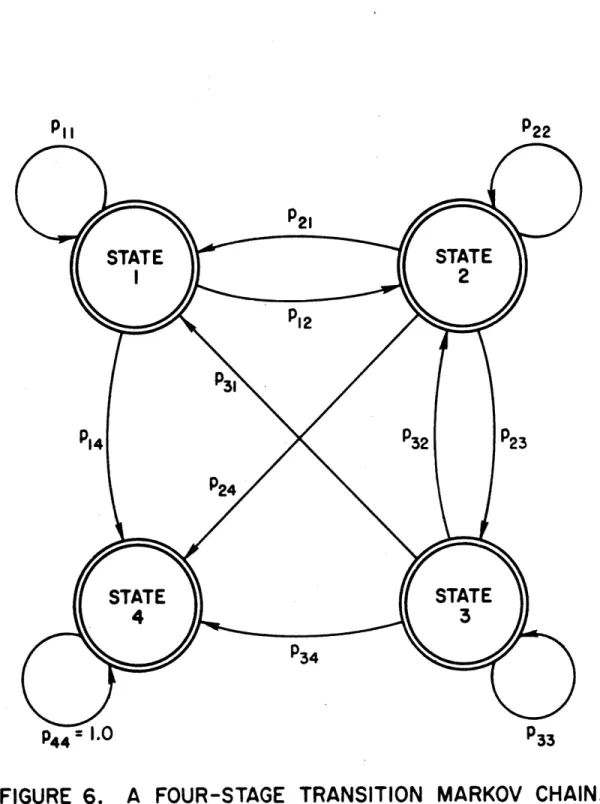
11.4.3. Markovian Behavioral Model for 60 Pavement Performance II.4.3.1. Introduction-Markov 60 Processes and Physical Interpre-tations 11.4.3.2. Serviceability Repre- 63 sentation in Markov Chains

11.4.3.3. Marginal State and 67 Transition

Prob-ability Assign-ments

11.4.4. System's Reliability 72

11.4.4.1. The Concept of Reli- 72 ability in Systems 11.4.4.2. Time-Dependent Reli- 74 ability of Highway Systems 11.4.4.3. Numerical Measure- 75 ments of Reli-ability

II.4.5. Life Expectancy and Distribution 77 of Times to Failure

11.4.5.1. Distribution of Times 79 to a Given State

11.4.6. Maintenance Activities and Modifi- 79 cations of the Markov Model

II.5. Summary 85

III.1. Scope III.2. Framework Model 111.2.1. 111.3. Method of 111.3.1. III.3.2. III.3.3. IV. Model IV.1. IV. 2. IV.3. V. VI. VII. VIII.

of the Maintenance Decision

Description of the Model

Approach

Multiattribute Utility

Analysis

Implementation of the

Decision Analysis

Numerical Example of Mainte-nance Optimization by Dynamic Programming. Page

88

89

90

108

Validation and Sensitivity Analysis Purpose

Description of the Computer Programs Sensitivity Analysis

IV.3.1. Influence of Geometric Factors IV.3.2. Influence of Materials'

Properties 113 113 113 118 118 126 133 144 146 149 149 151 156 160

IV.3.3. Quality Control Levels

IV.4. Summary

Summary and Conclusion

Recommendations for Future Research

VI.l. Field Verification and Model Calibra-tion

VI.2. Extension of the Existing Models Bibliography

Page

Appendix I - Detailed Stochastic Solutions of 163

the Model

Appendix II - Listing of Computer Programs 203 Appendix III - Tables of Ccmputer Inputs and Outputs for 238

LIST-OF FIGURES

Figure 1. An Overall Design Model

Figure 2. Flow Chart of the Structural Model Figure 3. Serviceability-Maintenance Model Figure 4. Operation of the Total Cost Model Figure 5. Distribution of Load Characteristics Figure 6. A Four-Stage Transition Markov Chain

Figure 7. Decision Flow Diagram for Maintenance Figure 8a. Midvalue Splitting Technique for Scaling

of Subjective Evaluation of Performance. Figure 8b. Performance Utility or Preference Curves

Obtained by Scaling

Figure 9a. Two-Dimensional Linear Indifference Curves for Tradeoffs between Maintenance Cost and Performance

Figure 9b. Four-Dimensional Indifference Curves for

Attribute Tradeoffs of the Multi-attribute Problems.

Figure 10. Utility Evaluation for the Multiattribute Problem

Figure 11. Influence of Geometry on Rutting History

Figure 12. Influence of Geometry on Roughness

Figure 13. Influence of Geometry on Crack

Progres-sion

Figure 14. Influence of Geometry on (a) Service-ability. Index, and (b) Reliability and

Life Expectancy

Figure 15. Marginal Probabilities for (a) Thin, (b) Medium, and (c) Thick Geometries

Figure 16. Influence of Material Properties on Rutting History Page 24 26 28 30 35 65 92 96 96 99 99 100 120 121 122 123 124 128

Figure 17. Figure 18. Figure 19. Figure 20. Figure 21. Figure 22. Figure 23. Figure 24.

Influence of Material Properties on Roughness

Influence of Material Properties on

Crack Progression

Influence of Material Properties on (a)

Serviceability Index, and (b) Reliability

and Life Expectancy

Marginal Probabilities for (a) Weak, (b) Medium, and (c) Strong Material Properties

Influence of Quality Control Levels on Roughness

Influence of Quality Control Levels on

Crack Progression

Influence of Quality Control Levels on

(a) Serviceability Index, and (b)

Reli-ability and Life Expectancy

Marginal Probabilities for (a) Poor, (b) Medium and (c) Good Quality Control

Levels Page 129 130 131 132 136 137 141 142

I. INTRODUCTION

Highway systems belong to a large class of public

facilities whose specific goals and functions are derived

from the more general goals of the society comprising the

users of the systems. The performance of these systems is largely dependent on the subjective evaluation of the users and their relative acceptability of the systems. It is

therefore desirable to evaluate these systems from the

stand-point of the levels of services they provide at any time during their operational life. In this context, failure

may be viewed as a threshold that is reached as the perform-ance level exceeds some unacceptable limits viewed by the

users of the facility.

The present design practices for highway systems are largely empirical, based on experience and engineering judgement. They are basically expressed in terms of

correlations between soil type, base course properties, thickness of the different layers, and traffic character-istics. Although these methods have met in the past with

moderate success, the rapid changes in traffic volume, in construction and maintenance costs and techniques, and the

use of potentially new materials make experience and emperi-cism obsolescent or totally lacking. Therefore, a design method which combines theory and empericism to a lesser

extent is needed. The method must encompass a set of analytical procedures that can effectively simulate the

behavior of the system and the interactions among its compo-nents. Further, this design method must choose as a means of system evaluation such measures of effectiveness that define the specific goals and functions of the system it represents.

I.1. Measures of Effectiveness

The analysis and design of pavements, similar to the analysis and selection of investment opportunity, require a knowledge of both the supply and demand functions involved. In this context, the supply functions may be considered

as a set of techniques available to combine a variety of resources to produce highway pavements. A set of resources combined in a particular way is referred to as a strategy. For example, a particular combination of certain types of material in a given geometrical configuration constitute one strategy. On the other hand, placing different types

of material in another geometrical configuration forms another strategy. Usually, there are several strategies that can

be acceptable for any situation. The question would be

which strategy meets the demand requirements most efficiently, where efficiency can be normally translated in economic

terms.

The demand function for pavements can be expressed in terms of the three components of performance; serviceability, reliability, and maintainability (S-R-M).

The level of performance or serviceability of any system, functioning in an optimal environment, is bound up by the uncertainties inherent in the.physical characteristics

of the system and in the surrounding environment. These uncertainties can be expressed in terms of the reliability of the system, i.e., the probability of providing satisfactory levels of performance at any point within the operational

life of the system.

Maintenance efforts exercised throughout the lifetime of the system controls the level of performance of the

system and its reliability, as well as its operational life. This may be expressed in terms of the maintainability, which

is a measure of the effort required to maintain adequate levels of serviceability throughout the design life of the system (L2)*.

Economic constraints play an important role in controll-ing the levels of serviceability throughout the lifetime of

the system by determining the initial costs, maintenance

costs, and vehicle operating costs.

1.2. Goal Formulation

The levels of (S-R-M) for each pavement should be

commensurate with the type of highway involved. For example

when the pavement is for an expressway, its levels of (S-R-M)

are quite different than those for a rural or suburban road. * The numbers in brackets refer to the list of references

For an expressway in a metropolitan area one demands a very slow rate of drop in its serviceability, a very high degree of reliability that something serious may not go wrong with the pavement, and a very low maintenance so that the traffic will not be disrupted. However in rural areas one may

tolerate lower reliability and more dependence upon mainte-nance for keeping the pavement operational. These variations in demand for the two cases are obviously dictated by the economics of the two roads. The monetary loss and social consequences of closing an expressway are more intolerable and expensive than those of rural road.

The design decision is then to choose the strategy which meets the demand requirements subject to certain con-straints. These constraints can be economic or otherwise. For example the constraint may be to choose the alternative which costs the least, or to choose one which needs minimum maintenance.

In order to be able to predict that a certain pave-ment system (a strategy) will meet the demand requirepave-ments, it is essential to have analytic or empirical means to assess how the given pavement system will perform in the specified environment and the projected loading conditions. Most empirical means (which, in the literature are erroneously referred to as methods of design) attempt to assess the performance capability of a given pavement system by simply evaluating a single response of the system. For example,

they indicate that a given pavement system will perform satisfactorily if a maximum allowable stress or deformation at certain points of the pavement is not exceeded. These maxima or limits are often set based on field observations

and past experience. Their application to other locality and their usefulness under a different set of circumstances have always been questionable.

Assuming that the "society" makes optimal use of its resources in deriving the maximum overall benefits for

any of its commodities, the overall objective in the design of highway system may be stated as: providing an economical riding surface at an"adequate" level of performance and

reliability for an optimum time period. Such adequate levels result in a structure which is reliable, safe in terms of comfort and frictional characteristics, and which will maintain some structural integrity at a low cost to the

"society" (M3, M4). The above statements define a goal

space from which a designer can derive his design objectives and requirements. In this capacity, the pavement designer is concerned with the description and selection of a set of optimal actions fulfilling the requirements imposed by

the goal space and constrained by the allocated resources. Moavenzadeh and Lemer (M3) provide a methodology for defining

a goal space for pavement design in the form of a hierarchi-cal structure. This structure can then be decomposed into less complex elements as a basis for search of alternate

goals and specific solutions (M4).

1.3. The Proposed Design Framework

This study presents a methodological framework for the analysis and selection of pavement systems suitable for a

given set of goals and constraints. A.set of models and

algorithms has been developed at two different levels of

analysis: analysis of the physical behavior of the system,

and analysis for the selection and optimization of a design

system. The first involves a set of mechanical and phenomeno-logical models which describe the response of the system in a realistic operating conditions of traffic and environment. From these models the progression of damage within the system

can be evaluated using some physical transfer functions. The second level of analysis utilizes the above information to determine the level of services that the system is providing at any time and the reliability of the system in the

operational environment. Maintenance policies can be gener-ated, and evalugener-ated, and an optimum set of strategies may be selected for a given design configuration over the

life-time of the system. Similarly, alternative design configur-ations can be generated and evaluated, and a framework for

the selection of optimum systems is presented based on cost criteria and users' constraints.

The basic features which characterize this study can be summarized as follows:

1. One particular feature of this study is that the proposed method of design for structural systems represents a departure from the

traditional cook-book style methods generally pursued in the literature. Instead, the

design is viewed as a process of sequential evolution of systematic analyses whose ultimate goal is the achievement of an optimal design configuration.

2. The criteria for model selection and evaluation are based on the users' subjective preferences for constructed facilities derived from their particular needs and sets of values. From this standpoint, the highway pavement is viewed as a system which is providing certain services to its users, and the quality of providing

these services must be evaluated from the users' demands and preferences

3. The models cover a wide spectrum of activities encompassing a large body of knowledge ranging from rational and applied mechanics to probability and operations research disciplines. The

particular advantage derived from this coverage is that it provides a means of continuity and integrity to the analysis and design. One can study for example the influence of change in geometry, physical properties, traffic patterns or quality control levels not only on the future behavior of the system, but also on its life, maintenance policy, costs, and so forth, through

4. The models possesses a causal structuring thereby defining the different interactions

between the system and the surrounding

environment. Also, the feedback processes

resulting from maintenance activities are accounted for.

5. The models recognize and incorporate the elements of uncertainty associated with the natural

physical phenomena and processes represented.

The following chapter deals with the development of

a set _{of models which are concerned with the prediction}

of the behavior of the system in the operational environ-ment. A structural model, based on mechanistic theories

is used for the analysis of the structural response of the system expressed in some physical manifestations of damage. These damage manifestations are similar to those developed by AASHO [Al] as the components of damage that the users

generally are sensitive to. The system itself is represented by a three-layer viscoelastic model with each layer having

certain statistical properties and geometry. A service-ability maintenance model utilizes the information provided

by the structural model to predict stochastically the

serviceability, reliability and life of the system allowing

for maintenance activities at desired time periods to be exercised to upgrade the system.

A framework for a decision structure for the choice of

configura-tion is presented in Chapter III. A dynamic programming-based algorithm is developed for this optimal selection.

Further a limited sensitivity analysis is presented in Chapter IV to validate and demonstrate the effectiveness of the developed models, which have been coded into a set of computer programs.

The development of further research activities to complement and calibrate these models in order that they

may be effectively used as practical design tools is discussed

II. AN ANALYTIC MODEL FOR PAVEMENT PERFORMANCE

11.1 An Overview

The development of a rational method for the analysis and design of engineering systems involves a set of procedures, of which the selection and analysis of a model or prototype for realistic inputs constitute a major part. A model, in this context, is an abstract representation of the form, operation, and function of the real or physical system (Dl). To provide such a model for design

purposes, it is essential that the system be characterized realistically; information about the design functions, behavioral interactions, and failure patterns and mechanisms must be provided.

The analysis of a systems-oriented problem requires the applications of certain procedures, each of which involves the use

of different methods and techniques for problem-solving and formulation. Therefore, the main problem at the outset of the analysis is that

of "proper" modelling. Different analysts may formulate different

models for the same system. It is not very clear whether the problem is that of formalism or that of abstraction. It is also possible that subjectivity and arbitrariness in definitions of the different aspects of formal problems may result in non-unique solu-tions to such problems. In any case, what follows is that subsequent decisions on the configuration of a certain design problem may vary considerably among analysts depending on the different interpretations

and valuation of the existing information. Since this is an

interpre-tations are based on a more objective source of information which may serve as a guide for one's actions and decisions.

One of the major objectives in the area of large-scale systems modelling is the construction of a causal model capable of handling the interaction of the different components of the system it represents. A causal model is one which is based on an a

priori hypothesis of the system's behavior as well as the interaction, within the system, of the different excitations and system's

characteristics. Such an interaction occurs in accordance with certain functional relationships which define the behavior of the

system and its responses in terms of some physical transfer functions. In general, most systems analysts require the following systematic procedures for the solution of systems-oriented problems:

1. Problem definition: which involves the determination

of the overall systems requirements, objectives, and constraints. Factors such as performance, reliability, cost, maintainability, and life expectancy are taken into account as measures of effectiveness for the evaluation of the system.

2. Generation of Alternatives: where several solutions are synthesized to form a solution space, which is scanned for the choice of a feasible solution.

3. Synthesis of the system: which involves the complete

4, Evaluation of alternatives: where the information

about the characteristics of the synthesized system is updated, possibly through simulation. In general, as the continuous process of evolution of the system proceeds, more and more emphasis is shifted from the theoretical representation of the system and placed on its physical aspects.

5. Testing of the system: where the characteristics of the resulting system are determined for the overall evaluation of the system.

6. Refinement of the design: in which the systems

requirements are correlated to the test data obtained above to re-examine the overall system interrelationship and reassess the contribution of its individual components

In this context, it may result that certain goals are not achievable and require further examination and

change (Sl).

This chapter discusses the development of a set of models for the analysis of highway pavement within its operational environment. The models are intended to be used in conjunction with the design of

pavement systems. In this context, the design process is viewed as a process of evolution of the analysis in which alternatives are synthesized

and evaluated for the choice of optimal design. The operational pol-icies encountered in the handling and maintenance of the system

are a part of this design methodology. The choice of feasible and optimal selections is based on a set of criteria which are partly subjective in nature and incorporate the users' demands and

aspirations for the systems at hand.

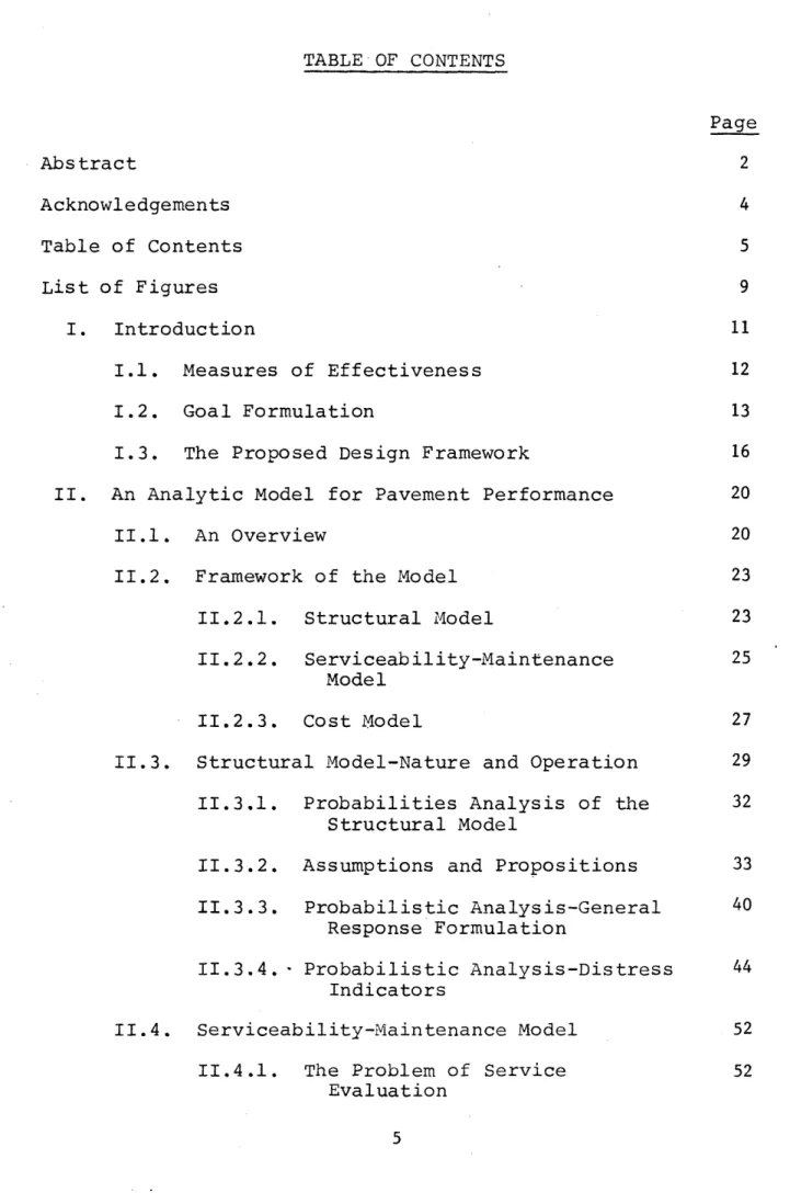
11.2 Framework of the Model

The general framework of the model may be described as a management-oriented framework. The overall model is viewed as

having three subsets of models which, when integrated together, result in a predictive structure for pavement design. These subsets are categorized into: structural model, serviceability-maintenance

model, and cost model.

These models and an optimization sub-model would then

provide a basis for the selection of an optimal system, among alterna-tive configurations and maintenance policies, based on some cost-effectiveness analysis.

The overall model developed in this study is shown in a block structure in figure (1). This thesis has been concerned with the development of the first two models which are discussed below.

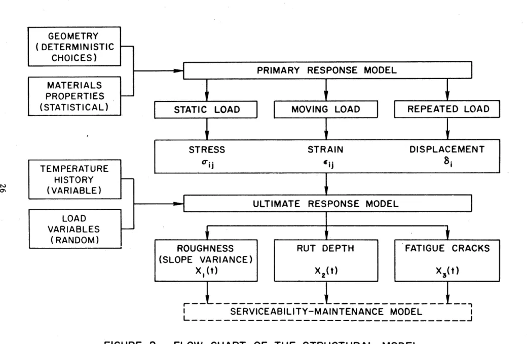
11.2.1 Structural Model

The structural model is concerned with the analysis of the structural response of the pavement systems. It provides information about the response and damage of the system with time. For analytical convenience, it has been decomposed into two stages: primary

response and ultimate response.

A three-layer viscoelastic model is used to represent the

pavement structure. This model is subjected to loading patterns similar to those of typical traffic patterns. The effect of climatic

I

STRUCTURAL MODEL

HIGHWAY COST MODEL

MAINTENANCE POLICY DECISIONS

SYSTEM OPTIMIZATION MODEL

AN OVERALL DESIGN MODEL.

SERVICEABILITY-RELIABILITY

SERVICEABILITY-

L.--MAINTENANCE

MODEL

_I

_MAINTENANCE

I

SUBMODEL

I

IJ

I,

I--FIGURE I.

variations in the form of temperature templates representing regional conditions are also accounted for.

In the primary response stage, statistical information regarding the response of the system to loads and environment is obtained. The response of the system is expressed in terms of first and second order moments of histories of stresses, strains, and deformations at any point within the layered system. (A2, El, Fl)

In the ultimate response stage, the primary responses of the system are expressed in terms of some descriptive, less objective damage indicators utilizing some probablistic transfer functions.

Such indicators reflect the user's perception and sensitivity to the quality of the system, similar to those developed by the AASHO Road Test (Al). These indicators define the surface quality of the system and are expressed statistically in terms of cracking and longitudinal and transverse deformation.

The structural model is depicted in Figure (2).

II.2.2 Serviceability-Maintenance Model

This model is in turn decomposed into two submodels: a

serviceability-reliability (S-R) model, and a maintenance model. In the S-R model, the distress indicators obtained from the structural model are combined in a regression form to provide a set of numerical valuqs indicating the levels of serviceability of the system and the user's relative acceptability of these levels. One form of such an equation has been developed by AASHO which

GEOMETRY

(DETERMINISTIC

CHOICES)

PRIMARY RESPONSE MODEL

MATERIALS

PROPERTIES

(STATISTICAL)

I

_S

TEMPERATURE

HISTORY

(VARIABLE) 0'

STRESS STRAIN DISPLACEMENT

'iijj I

F-

_{ULTIMATE RESPONSE MODEL}

_I

LOAD VARIABLES (RANDOM) -vUUnrlNto• (SLOPE VARIANCE)

X,(t)

X2(t)

X

(t)

FIGURE 2.

FLOW CHART OF THE STRUCTURAL MODEL.

FIGURE 2.

FLOW CHART OF THE STRUCTURAL MODEL.

I ATIC LOAD -1 I ~II~Ll~lr~~ 1 I ,

I

as the Present Serviceability Index (PSI). This equation has been reformulated in light of the uncertainty associated with the damage characteristics, and probabilistic estimate of the serviceability index are obtained at any desired time. From this, one can determine the probabilities of having any value of the PSI, referred to as the state probabilities. The probability, at any time, of being above some unacceptable value of the PSI is defined as the reliability of the system. This is a measure of the level of confidence that the system is performing its stipulated design functions as viewed by its users. In this context, the life expectancy of the system is deter-mined by the model based on its serviceability and reliability.

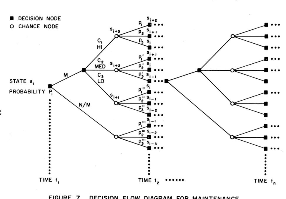
The maintenance model is aimed at introducing activities which result in improvements of the level of serviceability of the system, and at studying of the influence of such activities on the future behavior of the system and its life expectancy. In this model, strategies are generated over a range of time spectra, and their

subsequent effects on the serviceability, reliability, and life are determined at some associated cost estimates.

The serviceability-maintenance is shown in the flow

diagram of Figure (3). II.2.3 Cost Model

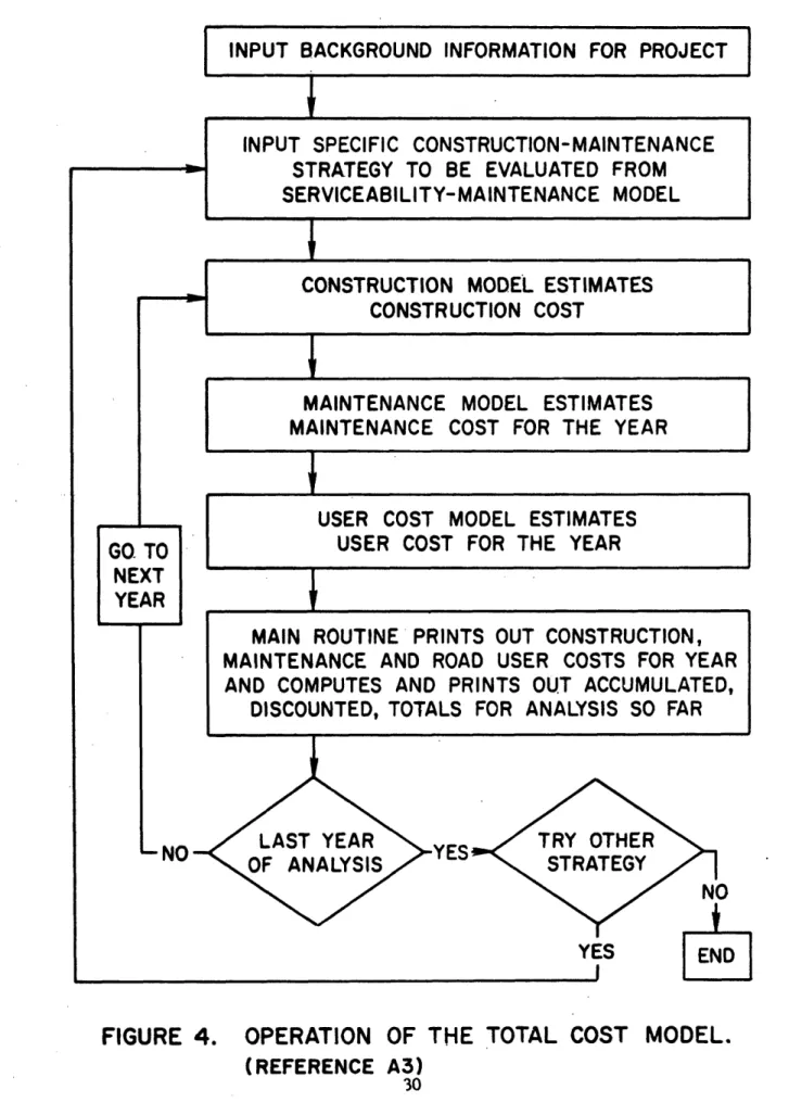
The cost model, which has been developed elsewhere (A3, Ml),

addresses itself to the determination of the total costs of construc-tion, operaconstruc-tion, and maintenance of highway systems. It incorporates three components: construction costs, roadway maintenance costs, and

ROUGHNESS

x,

(t)

X,(t)

SERVICEABILITY EVALUATION

PSI(t)

=

o

+

a,X,(t)

,(t)

+

aX(t)

STATE AND TRANSITION

PROBABILITIES

qi(t), Pij

MAINTENANCE STRATEGIES:

_Mi,

_{i = I,n}

AND RELIABILITY PREDICTIONS

HIGHWAY

_f

_---

_-COST

--

-MI

HIGHWAY COST MODEL

I_ -- - - - ---- - -- ---- - - - -- - -J LIFE EXPECTANCY AND

DISTRIBUTION OF TIMES TO FAILURE EXPECTED LIF_E u_ TIME RELIABILITY

aTIME

FIGURE 3.

_{SERVICEABILITY-MAINTENANCE MODEL.}

M,(ti)

M (ti)

vehicle operating costs. Each component in this model provides

estimates of the resource consumption, and yields the money costs of these resources using separately defined prices. Therefore, this model is adaptable to any economy regardless of the relative costs of different resources.

This model may be used in conjunction with the above models to provide a basis for decisions on the selection, operation, and evaluation of optimal design systems. The flow diagram in figure (4) depicts the nature of this model.

In the following sections, these models are discussed in details within the above framework, and the mathematical formulation and the related assumptions are presented. The cost model is not a part of this study, and therefore was not implemented as a part of the present analysis. However, the potentiality of integrating

it with the other models has been examined and few modifications may

be necessary to achieve an overall design system as was discussed earlier.

11.3 Structural Model-Nature and Operation

The structural model is a mathematical model of the pavement structure. It consists of a three-layer elastic or viscoelastic

system utilizing mechanistic theories for prediction of pavement response and distress. For analytical convenience, this model is divided into two stages: primary and ultimate. The primary stage has been developed by Ashton (A2) and Elliott (El) to yield stresses, strains, and deformation at any point within the layered system

with time under deterministic operational conditions. These conditions being (1) a static load applied in a step-form and kept for an

INPUT BACKGROUND INFORMATION FOR PROJECT

I,

CONSTRUCTION MODEL ESTIMATES

CONSTRUCTION COST

MAINTENANCE MODEL ESTIMATES

MAINTENANCE COST FOR THE YEAR

USER COST MODEL ESTIMATES

USER COST FOR THE YEAR

LAST YEAR

TRY OTHER

NOA YES

OF ANALYSIS

STRATEGY

NO

YES

FIGURE

4.

OPERATION OF THE TOTAL COST MODEL.

(REFERENCE A3)

30

INPUT SPECIFIC CONSTRUCTION-MAINTENANCE

STRATEGY TO BE EVALUATED FROM

SERVICEABILITY-MAINTENANCE MODEL

GO TO

NEXT

YEAR

MAIN ROUTINE PRINTS OUT CONSTRUCTION,

MAINTENANCE AND ROAD USER COSTS FOR YEAR

AND COMPUTES AND PRINTS OUT ACCUMULATED,

DISCOUNTED, TOTALS

FOR

ANALYSIS SO FAR

I

~

I

indefinite period of time, (2) a constant load moving along a straight line at a surface at a fixed velocity, and (3) a load repeatedly applied in the form of a haversine wave with fixed duration, amplitude, and frequency.

This earlier work has been modified to account for the realistic random nature of the operational environment. It is recognized that the behavior of pavement systems in an operational environment is largely a function of the intrinsic characteristics of the system, as well as the load and environment to which the system is subjected. Traffic loading is far from being predictable at any instance in time both in magnitude and frequency. Also, the climatic environment surrounding the system changes in a somewhat

random manner that can only be statistically defined and characterized. Similarly, the properties of the materials in the different layers vary considerably from one point to another due to variations in mixing and fabrication practices which introduce some inhomogeneities in the materials.

These uncertainties result in an unpredictable behavior of the system associated with probabilities of overload or inadequate capacity of the system to carry on its stipulated functions. With this frame of mind, a simulation approach was developed to account for these uncertainties under static loading modes (Fl). The inputs and outputs are described in this approach in terms of probabilistic distributions instead of single-valued estimates.

The present study utilizes the information obtained from the above simulation analysis to provide probabilistic estimates of

the history of response characteristics under randomly repeated loads and varying temperatures. The general probabilistic solutions mentioned above and the associated assumptions are detailed in the

following sections.

II.3.1 Probabilistic Analysis of the Structural Model

The following analysis is conducted for the case where loads are applied randomly on the system in a manner commensurate with actual vehicular arrival patterns in the real system. It utilizes the output of the simulation for the static load case, where a set of response functions are obtained in statistical formats, i.e., in terms of first and second order moments of the step function response. This response

may be viewed as a characteristic function for the total pavement system in which the contribution of all components is integrated as

a single response to a step function. This response can be expressed

in the form of an exponential series:

YijiGiexp(-t6i)

(2.1)

where ni is a random with a mean of 1.0 and a variance equal to the square coefficient of variation of Gi,*

G is the mean value of the random variable Gi, and 6i are the exponents of the series**, taken as deterministic quantities.

*Coefficient of Variation of Gi - V -i

Gi

**6 's are actually correlated to the retardation times of viscoelastic

To simplify the analysis considerably, .an assumption has been made in regard to q; that nl = n, for all i. This assumes that the response functions of the pavements to a step load are well

behaved and that they do not criss-cross each other due to variations

in the materials properties.

The terms in equation (2-1) are used as inputs to the next stage of the analysis, i.e., the repeated random loading mode. This state, as has been mentioned earlier, takes into consideration the fact that vehicular loads are applied randomly on the pavements with

varying velocities and intensities. It also utilizes the time-temperature superposition principle to account for the variations in the response due to change in temperature histories throughout the service life of the system. The effects of moisture have not been incorporated in the present study, but can be implemented in a manner similar to the temperature case.

11.3.2 Assumptions and Propositions:

Before turning into the formalization of the model, the assumptions that led to this analysis are discussed below. These assumptions may be divided into two categories: those related to the input variables, and those related to the output variables

A) Input Variables:

1. Traffic Load; The application of traffic load on a pavement system has been assumed as a process of independent random arrivals. Vehicles arrive at some point on the pavement in a random manner both

in space (i.e., amplitude and velocity), and in time (of arrival).

The arrival process is modelled as a Poisson process with a mean rate of arrival X . The probability of having any number of arrivals n at time t may be defined as:

p

(t)

exp.(=t)Gt)n

(2-2)

n no

Assumptions of stationarity, nonmultiplicity, and independence must be satisfied for the underlying physical mechanism generating

the arrivals to be characterized as a Poisson process (Bl). In this context, stationarity implies that the probability of a vehicle arrival in a short interval of time t to t + At is approximately A At, for any t in the ensemble.

Nonmultiplicity implies that the probability of two or more vehicle arrivals in a short interval is negligible compared to

X At.

Physical limitations of vehicle length passing in one lane on highway support this assumption; it is not possible that two

cars will pass the same point in a lane at the same time.

Finally, independence requires that the number of arrivals in any interval of time be independent of the number in any other

nonoverlapping interval of time.

In a Poisson process, the time between arrivals is exponentially distributed. This property is used to generate a random number of

arrivals within any time interval t.

The amplitudes of the loads in this process are also statisti-cally distributed in space. Traffic studies (D3) have shown that a

a

0q

-j

I fA~ II~~A ~ f%~\ A&t &mhh &Atz· hr r hi I F~ &

LVMLU M4rlWrVALZ lANU NUIUM~Irt UF" LUAUIU

NUMBER OF LOADS = 9

I

I

1I

I

T₁ T2 T3 T TT T6 T7 T T T 9 TIME, t

A. INDEPENDENT RANDOM ARRIVAL OF TRAFFIC LOADS

(A

POISSON PROCESS).

cr

_w

T, TIME BETWEEN ARRIVALS

B. EXPONENTIAL DISTRIBUTION OF TIME BETWEEN

CONSECUTIVE ARRIVALS.

DURATION OF THE LOAD - F(VELOCITY OF THE VEHICLE)

DURATION, D

DURATION, D

LOGNORMAL DISTRIBUTION FOR LOAD DURATION

AMPLITUDE OF THE LOAD - EQUIVALENT SINGLE WHEEL LOAD

DISTRIBUTION OF LOAD CHARACTERISTICS.

ft(d) z w

0I

w.

LOGNORMAL DISTRIBUTION FOR LOAD AMPLITUDES

logarithmic-normal (lognormal) distribution is suitable to represent

the scatter in load magnitudes. Means and variances of load amplitudes are used to represent this scatter.

The load duration, a function of its velocity on the highway, is also a random variable. In a typical highway for example, speeds may vary from 40 to 70 miles per hour. Accordingly, the load duration was assumed to have a statistical scatter represented by its means and variances from distributions obtained by traffic studies.

Figure (5) shows the statistical characteristics of typical load inputs to the model.

2. Climatic Environment: In this attribute, only temperature effects have been considered, with the assumption that moisture can be incorporated in a similar fashion at a later stage. Temperature variations from one period to another are accounted for through the time-temperature superposition of the response of the system. The variations within these periods.have not been considered due to the

complexities they introduce to the analysis. One can choose the time periods in such a way that averaging over temperatures within these periods can be justifiable. The present study allows for the study of hourly, daily, weekly, monthly, quarterly, and yearly intervals of time.

3. System Characterization Function: This set of inputs describe

the characteristic response of the total system to a step function, and is statistically described by a set of random coefficients (Gi) and

exponents (6.) of an exponential series of the form described by

equation (2.1) above. This is obtained by simulation of static load response, as has been discussed earlier in this section.

A typical response equation to a random load history and temperature history can be expressed by a convolution integral of the following form:

t

R[t-T, 0 (T)] = c[ (t)] + B[p(t)]

N

J[{il

-0

Si1 Gi exp (-S*T) dB [O(S)}] (2-3)

The second integral in this equation is only a corrective term and can be neglected for all practical purposes.

where: t

t*

I Y

(x)

dx

T

c, 8, and y are mapping parameters

for temperature effects in which:

= factor for vertical change of scale = 0 in

this study.

S = vertical shift factor = T(t)/T

y = horizontal shift factor

10** (.162 {T - T o)

T = reference temperature in *k t

_ (T) is a vector representing the temperature history

and R[ , ]: represents a vector for the system's response history

This response is expressed (through probabilistic transfer functions, which will be described below) in terms of the damage indicators suggested in the AASHO serviceability evaluation (Al). The propositions and assumptions made in this study for the evaluation

of these damage components are listed below..

b) Output Variables

The output variables are expressed in terms of two damage manifestations in the pavement structure: cracking and deformation. Deformation develops in the pavement in the transverse and longitudinal profiles of the pavement. One is manifested by the rutting in the

wheel paths of the vehicles, and the other in the roughness of the pave-ment longitudinal profile, measured by the slope variance of the

profile. The mechanisms of development of each of these damage.manifes-tations are described below.

1. Rutting: This component is assumed to be primarily

the result of a channelized system of traffic thereby causing differential surface deformation under the areas of intensive load applications in the wheel-paths. Given the statistical characteristics of the road materials and of the traffic, one can determine this

component, measured by the rut-depth, from the spatial properties of traffic loads. For a given traffic pattern, the split Poisson

property is invoked*, to obtain the differential surface deformation due to the channelization of the traffic.

*This property states that if a stochastic process is of the Poisson type with a mean of X, then the arrival pattern will still be of the Poisson type if there is a split or addition to the event sequence with a modified mean A'

2. Roughness: This component defines the deformation along the longitudinal profile of the pavement. To obtain some measures of roughness, information about the spatial correlation of the properties of the system must be obtained. This can be expressed in terms of the autocorrelation function of the surface deformation. This implies the assumption that roughness in pavement is mainly caused by the variations

in the properties of the materials and fabrication methods. One can relate the spatial variations in the materials to those in the surface deformation along the pavement profile. In this study, the slope

variance. as used by AASHO is used as a measure of roughness of the pave-ment, as will be described later in this chapter.

3. Cracking: Cracking is a phenomenon associated with the

brittle behavior of materials. A fatigue mechanism is believed to cause progression of cracks in pavements. In this study, a phenomeno-logical approach has been adopted, namely a modified stochastic

Miner's law for progression of damage within materials. This has been used in conjunction with a healing mechanism for viscoelastic materials at suitably high temperaturs. It is recognized, however, that a probabilistic microstructural approach based on fracture mechanics can provide a better substitute for the prediction of crack initiation and progression within the pavement structure.

Having reviewed the assumptions upon which the analysis in this study has been established, the basic formulations and analyses are presented in the following subsection.

11.3.3 Probabilistic Analysis - General Response Formulation

The following convolution integral can be used to represent the response of the system to load and environment:

t

R[t-T S)] = f(t T,#) dT (2-4)

where f( . ) represents the response function, and P(C. ) is the loading function.

For a haversine (sin2 wT) load, one can expand equation (2.4), with reference to equation (2.3') above as follows:

t

R(t) a- [O(t)] + 0[0(t)] I 1 -Gi exp(-t*6i)A(T)

0

Y

(T)

_D(T)

*{ Sinh 2 dT _(2-5)

Y(T) iD(T) 2

1 + [

2

Equation (2.5) may be broken into a sum of integrals over

(L) periods of time, each of which having a constant (average) temperature:

tk yk6iD(T) R(t) k1 L i -G A(T) Sinh 2 2 tklYk iD(I) k-1 1+

_21r

*exp

[-6

i {

(tkT) pk+1 Yp(tk-.-1)}]

(2-6)

Assuming that aOl(t)]

0

(2-7)

and since traffic loads arrive in a Poisson process integrally, there-fore equation (2.6) becomes:

sinh 2k61D k 2 R(t) =-kl E 1 1 [#(t)] GiAjk R(tk)9--l j=l i-l jk 6.D 2 + k iDjk 1+ 2

_27r

*exp [- k Yp tDEL

&i]

where:

Ajk = Load Amplitude

Dj - Load Duration

jk

nk total number of Poisson arrivals in the kth period

B( ) and Yk are temperature shift factors as defined in the previous section.

For simplicity of notation in further equations, let us call

-L B[C(tL)] (2-10)

The expected value and variance of the response of the system to a load excitation and temperature history of this derivation may

be found in Appendix I. This derivation follows from equation (2.8) which is a sum of "compound filtered Poisson processes". This is of the

Rk(t) == F<< W(tT,v) (2-11)

For which, Parzen [Pl] presents a general solution in terms of first-and second-order moments first-and correlations as follows:

E[Rk(t)] = E[(k(t,T,4)] dT (2-12)

-CcO

2

Var[Rk(t)] X

J

)j]

Cov[Rk(t),

R

(s)] = X

E[

(s,T,¶

) W (t,T,)l]dT

(2-14)

where, X is the mean rate of the Poisson arrivals.

The definitions for the terms in equation (2.12) through (2.14) and what follows may be found in Appendix I. From the above equations, as explained in the appendix, one can write

L

E(R(t)]

= -

E•[

Rk(t)]

(2-15)

Var[R(t)] - L Var •E Rk(t)] (2-17) L ri" 1

L

Var[R(t)]L = 2 {E Var [Rk(t)]

k=1l

L L

+ 2kz1 mk+l Cov[Rk(t), Rm(t)]} (2-18)

The analysis in Appendix I, yields the following solutions for (2-16) and (2-18)

L N

E[R(t)] = -BL k1 XA i 1 Gik Gi Vik ik (2-19)

Var [R(t)] = L2 k l a[+2{(2A + A 2)(I'_k +12

L L

2 3 -2 2

+•AI Ik}] + 2kEl +l (A + 2 )

N N

i-l j-i+l

i

j

ik jm 2

{[J2km -4km]km + 2(D)a2D}) (2-20)

where the second term in equation (2-20) is the

Cov [Rk(t), R9(t)]

All the terms and variables in equation (2-19) and (2-20) are

explicitly defined in the Appendix.

The nature of the response R(t) is derived from that of the systems characteristics Gi,6i, and r. If these represent the shear stress at the middle of the base layer resulting from a static

load; so does R(t) for random load and temperature histories.

Therefore, R(t) can be any of the time stress, strain, or deformation components aij' 'ij, and ui at any point. within the system depending

on the response function to a step load used as an input to equations

(2-19) or (2-20) above.

11.3.4 Probabilistic Analysis - Distress Indicators:

Through the assumptions listed in Section II.3.2 regarding the output variables, one can state the response R(t) in terms of the damage indicators mentioned above, as described below:

1. Rut Depth: This component is obtained through equations

(2.19) and (2.20) with a rate of traffic load A' described as follows:

A A c (2-21)

c N

where: XA is the proportion of channelized traffic in one lane. c

A is the total mean rate of traffic in the lane.

N is the number of possible combination of load channels in

lane in which the traffic passes (degrees of freedom). If, for example, 70% of the traffic is channelized at the center of the lane (i.e., XA = 0.7X), and there are three other

c

possible paths that the traffic passes through in one lane of the pavement, then

A - 0.7X

The values of Gi, 6i, and n are obtained by simulation of the vertical deflections at the surface of the pavement beneath the

center of a step (static) load.

These values with A' substituting for A in equations

(2-19) and (2-20) yield the means and variances of the rut depth

versus time.

2. Slope Variance: In the following analysis the spatial autocorrelation function of the surface deformation is obtained. From which, the slope variance can easily be obtained. The detail

of the mathematical work is shown in the second part of Appendix I. The spatial autocorrelation function of a system's

response Rt(x) may be expressed as:

Rt(x) - Ex[R(tx 0)R(t,x2)] -E[R(t,xo)] E[R(t,xL)] (2-22)

where E [ ] signifies that the expectation operation is taken over the space variable x, only and R(t,xj) is the response of the system at time t and location xj.

In this case, the response represents the vertical

deflection at the surface of the pavement measured at the center of the load as in the case of rut-depth measurement.

Equation (2-22) may be expanded as:

.

L

Rt(x) Ex

[{ k l

Rk(t,xo)}{Rk (txl)

L L

Since the roughness (expressed in terms of the spatial autocorrelation function) is a function of the spatial variation ý in the materials properties of the system, the only space variables in equation (2-23) will be n, which in this case can be written as nrx and rl or simply

n_o and ni, related to points x and zxX respectively.

The analysis in Appendix I results in the following expression: 2 L 2 Rt(x) = [p + _{l]( E} 1 k) (2-24) where Cov[ no S- 2 (2-25)

is the spatial correlation coefficient of the surface deflection in the pavement. The coefficient may be represented by the following expression:

Px

=A + B

exp

[-

jxf2/C

]

(2-26)

where xI = ox - x lis the absolute distance between the two

points = x

A is the minimum correlation between points far

apart from each other. It may be compared with 'the endurance limit in fatigue curves.

and B and C are materials properties.

If equation (2-26) is substituted in equation (2-24), we

get L

Rt

[A + B exp -2

+]

(k1

Zk

-E[R(t,x_o )] E[R(t,x )] (2-27)

Define Z(t) as the first space-derivative of the function Z(t), i.e., x- [i(t)], and if S(t) represents the vertical surface deformation, then S(t) will be -x [S(t)], which is the slope of the

surface as a function of time. Since:

2

a

ZX

R

(2-28)

s(t) 2 _x

2

where a 2(t) is the variance of the slope S(t), i.e., the

slope variance as defined by the AASHO Road Test, and

2-2R t(x)

ax2

x

i

0

represents the second space derivative of the autocorrelation function

evaluated at x * 0

Equations (2-27) and (2-28) yield:

L 2

2 2B 2

Slope Variance = (t) k 1 Zk) a (2-29)

where Z_k is defined in Appendix I. 2

Since a is a random variable in time because of the randomness in the load history, one can find-the expected values and variances of this variable versus time as shown in the

Appendix.

These are expressed as:

2 2 L

E[G2 ] 2Ba k 1 A+ A2 +1

C(t) 2 L =1 A k k

C k

L L

Var (a((t)] • B L k 1 Var [Z k(t)] (2-31)

The terms in equations (2-30) and (2-31) are defined in the appendix.

3. Cracking: A phenomenological model is used for the

prediction of the extent of cracking in the pavement structure. This is based on Miner's hypothesis for damage of materials. The criterion for cracking used in this study is based on fatigue resulting from the tensile strain at the bottom of the surface layer.

This requires the determination of the moments for the radial strain amplitudes at the bottom of the surface layer, using the radial strains obtained for step functions from the static load

program. These moments for the strain amplitudes may be determined from the following equations*:

_YM iD N G [1 + exp{ 2 ] 2i + 27 ) 2ir (2-32)

where Ac represents the radial (tensile) strain amplitude.

The mean and variance of AE_M have been obtained by the

probabilistic analysis in Appendix I, and can be written as:

N G [1 + exp(-YM.iD/2)]

E [AI ] = a- A

-2·rr

N YM6i . exp (-YM 6D/2)(1 + 2

1 2 M M + -

₄

D

i=1

_i

₂

_YM

6

_ID

₂

1 + (1 - VMiD/2) exp(-yM6_iD/2)

Y( 6'ib 2 2

(1+

- ) }

2(1 + exp (-YM6iD/2)

i2 YiD 2 3

(1 + (----

₂₂₎

(2-33)

Var[A%₁]=

a

[1 +

(YM•i

_2-ff

Gi[1 + exp(-yM6ID/2)]

(1 + ( YiD 2 D (ij= Gi

[1

+

exp(-yMSiD/

1

1 + ( 27)

YM61i

-M

_i

2

26

-2

Miner's law can be expressed as:

L nk Nk

D(t) NE (2-35)

k=1 k

Where D(t) is the damage at time t, resulting from a repetition of loads over L periods of time.

(2-34) __

-Nk represents the number of loads to failure at the kth

period, having the same statistical properties as the nk loads. The ratio nk/Nk represents the proportion of damage in terms of fatigue cracking in the kth period.

A fatigue law has been used to determine Nk, the number

of loads to failure in the kth _{period in terms of the tensile}

strain amplitudes obtained above.

1 a(T)

N_k C(T) ) (2-36)

kC(T)

where (c) and (a) _{are material characteristics of certain statistical} properties, which are temperature dependents.

Appendix I, under the subheading "Probabilistic Formulation of Minor's Law" presents the analysis to obtain the expected value and variance of Nk, and eventually, the expected value and variance of the damage D(t) versus time. These are:

E[D(t)] = _L k -k 2 (2-37)

1 +N _{3E[D(t) k}

where n_k is the mean number of Poisson loads in the kth period.

Nk is the mean number of loads to failure in the kth period and

a2 is the corresponding variance.

a2

L nk "k 2 Var [D(t)] =k+1 [ _+(2-38)

Nk2

where o2

is the variance of traffic loads in the k h _{period - nk}

k

for a Poisson process.

The above damage indicators have been expressed in algorithmic forms and are obtained readily by computer analysis to be used in the next step in the system of hierarchy of the present analysis, namely to determine the serviceability of the system with time and the associated reliability and life expectation.

II.4 Serviceability--Maintenance Model 11.4.1 The Problem of Service Evaluation

Traditionally, the services provided by a highway pavement have been tacitly described in terms of some manifestations of

deformation and disintegration. These manifestations have often been arbitrary as to the limits they impose upon what constitutes

satisfactory service, and have been developed usually from empirical and rule-of-thumb practices. Most of the present pavement design practices, for example, take into consideration the load bearing

characteristics of the pavement in terms of the maximum allowable stress or deformation as the only design criterion. However, it is widely recognized that surface characteristics of the pavement

have important effects upon the road's adequacy as a transportation link in terms of safety and ride, which are not accounted for in these design methods.

The AASHO Road Test provided one of the early recognitions that a pavement is providing a transportation service and must be analyzed in broader terms. The adoption of the term "present

serviceability" to represent the ability of a pavement to serve traffic,

and the interpretation of service as deriving from users' response represented a break with previous practice. Yet even in its

formula-tion, the AASHO approach is restricted to consideration of pavement surface riding quality. It neglects such factors as maintenance

and safety features of the road.

The user of a highway as the recipient of the benefits of transportation, provides a link between the highway and the social, political, and economic systems which the highway serves. The pavement must be viewed as a part of a transportation system, and if the pavement is to fulfill this role, it must provide service to the user. That is the evaluation of a pavement's physical behavior must be made in terms of users' wants and needs.

11.4.1.1 Measures of Effectiveness

It has been suggested that the term serviceability may be defined as the degree to which adequate service is provided to the user, from the user's point of view (L1, L2). Implementation of this concept as a measure of effectiveness for decision making

provides a translation of the requirements of the larger role of the pavement into terms of physical importance. For pavements, service-ability is represented by three components: rideservice-ability, safety, and structural integrity.

Rideability refers to the quality of ride provided by the pavement, and is measured by the users' response. Included are such factors as comfort and likelihood of damage to goods. Safety depends upon skidding characteristics of the pavement and the

presence of such things as obstructions and glare spots which might 53