Design optimization of parabolic arches subject to non-uniform loads

(1)

DESIGN OPTIMIZATION OF PARABOLIC ARCHES SUBJECT TO

NON-UNIFORM LOADS

by

Lavina H. Sadhwani Bachelor of Science in Civil Engineering University of Illinois at Urbana-Champaign

May 1998

MASSACHUSETTS INSTITUTE OF T ECHNOLOGY

MAY 3 0 2000

LIBRARIES

SUBMITTED TO THE DEPARTMENT OF CIVIL AND ENVIRONMENTAL ENGINEERING IN PARTIAL FULFILLMENT OF THE REQUIREMENTS FOR THE DEGREE OF

MASTER OF ENGINEERING

IN CIVIL & ENVIRONMENTAL ENGINEERING at

MASSACHUSETTS INSTITUTE OF TECHNOLOGY June 2000

The author hereby grants MIT permission to reproduce and distribute publicly paper and electronic copies of this thesis document in whole or in part.

Signature of Author I'_FW

Pepartment of Civil and Environmental Engineering May 5, 2000

Certified by

Jerome J. Connor Professor of Civil and Environmental Engineering Thesis Supervisor

Accepted by

Daniele Veneziano Chairman, Departmental Committee on Graduate Studies

(2)

Lavina H. Sadhwani

Submitted to the Department of Civil and Environmental Engineering on May 5, 2000 in Partial Fulfillment of the Requirements for the Degree of

Master of Engineering in Civil and Environmental Engineering

Abstract

Arch structures have been used for centuries in various types of structural systems, particularly buildings and bridges. Arches are characterized by the ability to carry load primarily through axial action. An arch shape can be optimized such that the design load pattern is carried by purely axial action. If the load pattern on the optimized arch differs from the design loading, bending stresses develop in the arch. Load carrying mechanisms that resist load through bending are less efficient than systems that resist load through axial

action. An active control system on an arch can be used to reduce the bending stresses in an arch. Control forces, and resulting moments are applied to counteract moments produced various other load

combinations. The actuator, a component of the active control system, imposes counteracting control moments on the arch to limit the resultant moment forces in the arch to a pre-defined limit.

This thesis includes a description of basic arch theory; specifically, a description of various types of arches, force equilibrium equations for arch structures, and the theory behind design optimization of arch shapes for a design load pattern are presented. Additionally, the fundamentals of active control systems, including components of the system and a basic algorithm are discussed. A case study is then utilized to demonstrate that an arch structure enabled with an active control system can carry all load patterns mainly through axial action.

Thesis Supervisor: Jerome J. Connor

(3)

ACKNOWLEDGEMENTS

Writing this thesis would have taken a lot longer and been a lot more difficult if it wasn't for a few people who provided me with guidance and support, both professionally and

personally:

Professor J.J. Connor, for his guidance and advice. More importantly, for revitalizing my enthusiasm for

my career in structural engineering.

Emma Shepherdson, for helping me get started.

Frank, D.J , and Brant, my eternal appreciation for listening to my continuous nagging and whining and

for helping me with my formatting issues.

George Kokosalakis, for his assistance with the MATLAB program. Myfamily, for their continuous support and encouragement.

(4)

Table of Contents

Abstract 2

1.0 Arch Structures 6

1.1 Types of Arches 7

1.2 Arch Theory 8

2.0 Funicular Method of Arch Design 11

3.0 Disadvantages of Traditional Arch Design 12

4.0 Active Control 13

4.1 Components of Active Control System 13

4.2 Actuator Technology 15

4.3 Active Control Algorithm 16

5.0 Active-Controlled Arch Structure 18

6.0 Design of Proposed Charles River Crossing Bridge Arch 19

6.1 Introduction 19 6.2 Loads 20 6.2.1 Superstructure Loads 21 6.2.2 Self-weight 23 6.3 Funicular method 24 6.3.1 Determination of Constraints 24

6.3.2 Determination of optimal arch shape 25

6.4 Computer Model 25

6.5 Optimized Arch Shape 27

6.6 Discussion of Design Stresses 28

7.0 Design of Active Control System 29

7.1 Configuration of Actuators 29

7.2 Active Control Algorithm 30

7.3 Results of Active Control Algorithm 31

8.0 Conclusion 34

(5)

Table of Figures

Figure 1: N ew River G orges Bridge... 6

F igure 2: N atchez B ridge ... 7

Figure 3: Oudry Mesly pedestrian bridge... 8

F ig ure 4: Typ ical A rch ... 9

Figure 5: Equilibrium Force Equations for an Arch... 9

Figure 6: Components of an Active Control System...14

Figure 7: Three-rod Actuator scheme ... 16

Figure 8: Proposed Charles River Crossing Bridge ... 19

Figure 9: SAP2000 M odel of Arch ... 23

Figure 10: Required Geometric Dimensions for Arch... 24

Figure 11: Optim ized Arch Shape ... 27

Figure 12: Moment Diagram ofArch under Design Load Combination (1)... 28

Figure 13: Moment Diagram of Arch under Critical Load Combination (3)... 28

Figure 14: Interaction Diagram for Critical Section... 29

Figure 15: Proposed Actuator Scheme on Arch... 30

Figure 16: Graph of Critical Design Moments (Md) and Target Control Moment Distributions (M c *) ... 3 1 Figure 17: Graph of resulting Control Moments (Mc) and sum of moments on structure (e)... 32

Figure 18: Interaction Diagram of Critical Section of Arch... 32

MASSACHUSETTS INSTITUTE OF TECHNOLOGY Page 5 of 50Page 5 of 50 MASSACHUSETTS INSTITUTE OF TECHNOLOGY

(6)

1.0 Arch Structures

The first true arch structure was built approximately 44 centuries ago. However, it was not until 44 centuries after the construction of the first arch that the mechanics of arches was completely understood and formulated in the elastic theory of arches (Spofford,

1937). The enduring use of arches in civil engineering structures is attributed to the aesthetic appeal and the structural efficiency of the system (Melbourne, 1995). The first constructed arches were made of masonry. With masonry construction, the longest arch structure spanned 300 feet. With the advent of more sophisticated materials, specifically steel and reinforced concrete, arch spans have increased (Spofford, 1937). The New River Gorges Bridge, is a 1700 feet metal arch bridge located in West Virginia; currently, it is the longest constructed arch (Figurel). The longest concrete arch bridge is located in Krk, Croatia and spans 1280 feet. The Natchez Bridge, is the longest concrete arch bridge in the Unites States; it is located in Franklin, Tennessee and consists of two spans, with the longer of the two arches spanning 582 feet (Figure2).

Figure 1: New River Gorges Bridge

MASSACHUSETTS INSTITUTE OF TECHNOLOGY Page 6 of 50_{Page 6 of 50} MASSACHUSETTS INSTITUTE OF TECHNOLOGY

(7)

Figure 2: Natchez Bridge

1.1 Types of Arches

There are three basic types of arches, a hingeless (fixed) arch, a two-hinged arch, and a three-hinged arch. Older masonry arches have fixed supports at each base. The

corresponding six unknown reactions make fixed arches statically indeterminate

structures. The use of modern construction materials has made the possibility of structural determinate arches a viable alternative. A three-hinged arch incorporates a hinge at the crown of the structure in addition to hinges at the supports. The advantage of three hinged arches is they are statically determinate and can be solved through equations developed by the elastic theory; however, arches with fixed pinned supports are less stiff than structures with fixed supports. A two-hinge arch, which is also statically determinate, incorporates hinges at the supports, thereby preventing any moments from developing at the supports. For the special case where the arch loading and configuration are perfectly symmetrical, all types of arches can be also be solved through elastic equations. (Spofford, 1937)

A tied arch, incorporates an additional tension member that (typically) spans between the abutments. This member resists the horizontal thrust, thus the foundation needs only to resist vertical reactions. The tension tie must provide sufficient stiffness and prevent the arch from displacing excessively.

Page 7 of 50 MASSACHUSETTS INSTITUTE OF TECHNOLOGY

(8)

Most constructed arches consist of an arch spanning below the point of load application. More recent arch structures have incorporated the arch above the point of load

application. The Oudry Mesly pedestrian bridge in Paris, France is an example of such a structure (Figure 3). The rationale behind the placement of the arch is related to the desired aesthetics and allowable clearances.

Figure 3: Oudry Mesly pedestrian bridge

1.2 Arch Theory

The distinguishing feature of an arch relative to other load carrying systems is that it carries vertical loads primarily through axial action, and not flexure. Axial action is a preferred load resisting mechanism since it makes the most efficient use of the

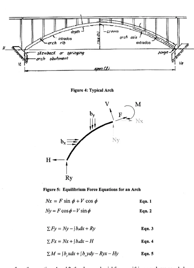
construction material. Figure 4 demonstrates a typical arch, including the pertinent features. The arch shown in Figure 4 is a two-hinged arch. Governing force equilibrium equations for arches are shown below Figure 5.

(9)

DESIGN OPTIMIZATION OF PARABOLIC ARCHES SUBJECT TO NON-UNIFORM LOADS

lam(I

Figure 4: Typical Arch

V M

Ry

Figure 5: Equilibrium Force Equations for an Arch

Nx = F sin

#

+ V cos

#

Ny = F cos -V sin# I Fy = Ny - J b,dx + Ry ZFx = Nx + J bxx - H E M = fbxdx + J bxydy - Ryx - Hy Eqn. 1 Eqn. 2 Eqn. 3 Eqn. 4 Eqn. 5

As seen from the equations 1 and 2, the shear and axial forces within an arch are coupled. As a consequence, under purely vertical load or purely horizontal load, both vertical and

bX

Page 9 of5 MASSACHUSETTS INSTITUTE OF TECHNOLOGY

(10)

horizontal reactions must be resisted at the foundation. This behavior is unlike typical beams; a beam loaded with purely vertical load only resists vertical reactions at the supports.

Although the arch equations allow for an arch to experience shear, bending, and axial stresses, an optimized arch will experience primarily axial compression under load. Specializing equation 5 for the case where no moments are allowed in the structure, and assuming the arch is not subjected to any horizontal loads, the following equation results.

f by xdx - Ryx

y Jx)= _H R Eqn.6

where y(x) represents the required distance between the springing (or tension tie) to the centerline of the arch. The numerator in equation 6 is the exact expression for the moment in a simply supported beam; the denominator is the value of the horizontal reaction. From this equation, one can see that an optimized arch, i.e. one that experiences no bending, is a scaled version of the moment diagram of a simply supported beam subject to transverse loads.

In order for the optimized arch shape to be symmetrical, the applied loading must be symmetrical. To attain a symmetric and parabolic arch curve, the design load must be a uniformally applied vertical load loading throughout the arch. Fortunately, a series of equal point loads equally spaced will also yield a symmetric shape that is nearly parabolic; however, the resulting shape will not be a smooth curve. If the load on a parabolic arch is not symmetric, or if the load pattern does not conform to the bending diagram of the optimized shape, the arch will experience bending. The critical load pattern for an arch is the case where only half the span is loaded. Under this condition the maximum moment develops at the quarter point of the arch.

MASSACHUSETTS INSI IIU'JiE Ut' IE(JHNULU(iY Page IU ot ~U_Page ₁₀ _{of 50}

(11)

2.0 Funicular Method of Arch Design

For every load pattern on an arch, there exists an optimum arch shape, for which the applied loading is resisted through purely axial action. No bending stresses exist in the arch under this condition. There are several procedures used to determine the optimal arch shape. All these procedures are based on the same objective: no moment in the arch. For a given load configuration, there are an infinite number of optimal shapes. A

particular solution is generated by specifying a constraint, such as the arch length, three pre-determined points along the arch, or the thrust force (Allen, 1998).

A funicular method of design, a graphical or numerical procedure, derived from equation 6, is used in this study to determine the optimum arch shape. The wordfunicular comes from the Latin word, funiculus, meaning "string." (Allen, 1998) A funicular shape is the form a piece of string would take under an applied load. Similar to a string, a funicular shape resists load through axial action. A piece of string supporting uniform loads or equally spaced concentrated loads takes the form of a parabola. Thus, a parabola is the optimal shape for a structure resisting uniformly applied vertical loads through axial action. (Heller, 1963).

The procedure, specialized for the constraint of three pre-determined points that the arch must pass through, depends on the fact that the horizontal component of the force, Nx, at each section of the arch is constant. This horizontal force is also equal to the thrust at the foundation.

The first step in the funicular method is to determine the moment diagram (or

distribution) along the arch due to all vertically applied loads, including the self-weight of the arch. The self-weight of the arch is typically not known during this first step. Thus, for the first design iteration, a self-weight distribution is assumed. The moments are

Page 11 of 50

(12)

summed on a horizontal projection of the arch length. That is, the arch is assumed to be a simply supported beam. To determine the value of the constant horizontal force, Nx, the moment force at one constrained location is divided by the established distance between the arch centerline and the springing. The required distance from the arch centerline to the springing for every other point along the arch is found by dividing the moment at that particular section by Nx. (Allen, 1998)

3.0 Disadvantages of Traditional Arch Design

Further study into the funicular method and equation 6 identifies an important

disadvantage of arch design: an arch shape is only optimizal for a particular load pattern. If the distribution or magnitude of the loads are altered, the stresses along an arch change; thus the arch shape will need to be altered for optimal conditions. However, arches are static structures and it is unrealistic to change the structural geometry according to transient load patterns. Consequently, traditional arch design utilizes the dominant load configuration to determine the arch shape. For arch bridges, the dominant load (the design load combination) is an arch loaded with full dead load and half the design live load. For most other arches, the dominant load is an arch loaded with full dead load. Under these conditions an arch will have purely axial action. It is usually under other load cases, particularly live load that arches experience bending.

Depending on the arch structure, the bending due to secondary load cases may be significant. The need to design an arch to resist bending in addition to axial loads diminishes the attractiveness of arch structures. A more efficient arch design incorporates a mechanism to limit the bending stresses in the arch to a pre-defined allowable limit. Active controls applied to an arch provides an example of how efficiency of a structure improves with the application of external control devices.

MASSACHUSETTS INS~'i FLUTE UP I ELHINULU~Y rage IL 01 DU

(13)

4.0 Active Control

A significant amount of inefficiency in structural systems results from the need to design a structure for all possible design load conditions. Further, this type of structural design is contingent upon always having reliable knowledge of the relative magnitude of all loads the structure that will be applied to the structure (Connor, 1999 ).

The introduction of passive mechanisms of control has increased the efficiency of structures by preventing loads from entering a structure, as in the case of base isolators used to isolate a structure from seismic ground accelerations. Damping systems are also utilized to dissipate the amount of energy, and therefore, stresses and movement the structure experiences from dynamic loads. The shortcoming of these systems is that they too are dependent on reliable knowledge of expected forces the structure will experience. Both these devices are designed according to expected forces. (Connor, 1999)

The benefit of active controls is that they can accommodate unexpected loads imposed on a structure. Active control devices are designed to monitor structural variables, such as forces and displacements the structure is experiencing. The mechanism then determines if the displacement or force exceeds pre-defined limits. In this case, the system determines a set of actions that will change the structural state to an acceptable one. An actuator, a mechanical device, induces a force or displacement according to the determined actions to counteract externally applied forces or displacements (Connor, 1999).

4.1 Components of Active Control System

Active control devices are composed of three main components: the monitor, the

controller, and the actuator. The monitor is a set of sensors located along the structure

used to monitor structural variables discussed above. The controller is a cognitive module, in some cases, with adaptive learning, which analyzes the sensor readings and

Page 13 of 50

(14)

uses a control algorithm to determine what actions to take to limit the forces or displacements. The actuator implements decisions made by the controller. All the

components depend on an external energy source to investigate and implement decisions. Figure 6 demonstrates the relationship and interaction between the components of an active control system. (Connor, 1999 )

EXCITATION STRUCTURE RESPONSE

ACTUATOR

MO0NITOR MONITOR

to gure DEV:LopTHE ACTION PLAN ControlSStem

external f th C l as o omue

loading a T Wit tAhiknown response

| DECIDE ON COURSE OF ACTION

.|DENTIFY THE STATE OF SYSTEM

-CONTROLLER

Figure 6: Components of an Active Control System

Since force actuators require time to apply the force, the controller must have the

capability to predict forces a short distance off from the actuator. In the case of a bridge, this scheme can be implemented if the controller was able to compute the weight and velocity of a load moving along the deck. With this known information, the controller can predict the impact of the load on the structure and send a signal to the actuator to apply a counteracting force to maintain the forces in the arch to a prescribed limit. (Connor, 1999)

Current technology is able to support the sensors and algorithms required for the controllers. However, actuator technology requires further advancement before active control technology can be applied to large civil structures. Civil structures generally require actuators to deliver large force to a system and to have short response times (generally on the order of a few milliseconds). There are a number of different types of

Page 14 of 50

(15)

actuators that can impose a large force on a system; however, these actuators have long response times. Most actuators require a large amount of energy to deliver the required forces. Before active control technology can be implemented in civil structures, actuators that are capable of delivering thousands of Newtons of force to a system within a few milliseconds without requiring a large amount of external energy must be developed. Alternately, the cost and ease of installing the system must improve so that multiple actuators can be installed in a structure. (Connor, 1999)

4.2 Actuator Technology

There are three types of actuators technologies: hydraulic, electro-mechanical, and electro-magnetic linear actuators. Each type of actuator has two components, a piston and a gear mechanism. The gear mechanism applies a force to the piston in order to translate the piston. Consequently, the piston applies a force to the structure and a reaction force is felt be the gear mechanism. In cases where there is not adjacent surface to absorb the reaction from gear mechanism, a self-equilibrating actuator system is utilized. (Connor, 1999 )

An ideal actuator system is one that can deliver a large amount of force in a small duration of time using minimal external energy. To control moment distributions on a structure linear actuators must be place below or above a structure. One

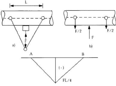
self-equilibrating actuator scheme, applicable to the arch structure, is composed of three rods and a gear mechanism (see Figure 7). (Connor, 1999)

MASSACHUSETTS INSTITUTE OF IEGHNULU(Y rage _{Page 15 of 50}is at 50

(16)

L |+ - - - +

b)

A R

FL/4

Figure 7: Three-rod Actuator scheme

The vertically applied load F is equilibrated by vertical component of the force in the diagonal rods. The forces cause a triangular moment field. A compressive force, of magnitude F/2 is induced in the localized area. The shear force in the localized area is also expected to increase. With a number of these actuator-rod configurations placed in series, one can generate a piece-wise linear bending moment distribution.

4.3 Active Control Algorithm

The first step of determining the active control algorithm is to set a pre-defined limit on the allowable stresses the system can withstand. For the case where moments need to be

controlled it is necessary to specify the maximum allowable moment, M(x)*.

The moment a structure feels at any point in time is the sum of the moment due to dead, live, or other loads, Md, and the moment caused by the active control, M.

M* > M(x) = Md(x) + Mc(x) Eqn. 7

MASSACHUSETTS INSTITU'I E (91- IELI-INULO(iY Page _{Page 16 of 50}lb 01 iU

(17)

The design objective is to limit M(x), the moment at any point in the structure, to M(x)*: Using matrix notation, this simplifies equation (7) to the following:

- Md - M* < Mc & M * -Md Eqn. 8

From the range of acceptable control moments, Mc, one generates the target distribution, Mc*. The sensor on an active control system senses the forces or moments at specified

locations on the structure. If the number of actuators on the system (r) is equal to the number of sensor locations (n), the algorithm for the active control simplifies to applying the actuator load to induce MC* at the sensor location. In this case, MC* will always be

equal to Mc. In most cases, the number of sensors on the system exceeds the number of actuators (n>r). In this case, it is not possible to obtain the exact value of Mc* at every sensor location. In this case, MC is a linear combination of moments caused by several actuators. (Connor, 1999)

Mc ='Tm Eqn. 9

The error between Mc* and Mc is designated by e:

e=Mc*-Mc=Mc*-'Pm Eqn. 10

y is a vector of size nxr, which represents the distribution of moments due to a single actuator; m represents the maximum magnitude of the moment field. In the case, where the number of sensor exceeds the number of actuators, the goal of the control algorithm is to minimize e using a least square algorithm. The least square method can be used to determine an appropriate solution for e = 0. The error measure is taken as the norm of J (Connor, 1999):

J=-eTe Eqn. 11 2

MASSACHUSETTS INSTITUTE OF IELHNULUUY 1'age 1/ at Page 17 of ~U50

(18)

Requiring J to be stationary with respect to each moment parameter contained in m leads to a simple matrix equation

am =b Eqn. 12

am

where,

a = T T Eqn. 13

b=T Mc* Eqn. 14

5.0 Active-Controlled Arch Structure

Active control implemented on an arch structure is an ideal application of the

technology. With active controls, the arch shape and sections can be designed to carry the dominant design load pattern through axial behavior. Rather than designing the arch to resist stresses, particularly those produced by bending, caused by additional load cases,

other load cases will be supported by adjustments made be the active control mechanism. The benefit of this system is an arch structure that primarily carries axial load and a minimal amount of bending, regardless of the load configuration.

MASSACHUSETTS INSTITUTE OF TECHNOLOGY Page 18 of 50Page 18 of 50 MASSACHUSETTS INSTITUTE OF TECHNOLOGY

(19)

6.0 Design of Proposed Charles River Crossing Bridge Arch

Figure 8: Proposed Charles River Crossing Bridge

6.1 Introduction

Components of the applicable design conditions and criteria of the proposed Charles River Crossing Bridge (see Figure 8) will be utilized in this study. Active Control theory will be implemented in the design procedure to demonstrate the reduction in bending stresses in the arch under critical load conditions. The proposed bridge, a 750-foot span, segmental, pre-cast concrete, two-hinge arch bridge is seen on Figure 8. The rise of the proposed bridge is 250 feet from the waterline. A unique feature of this bridge is the location of the tie. Typically, the tie on an arch is located at the foundation level. Since the bridge spans over a water crossing, the tie had to be placed at higher elevation. Currently, the tie is at deck level and braced by the deck superstructure. The arch is constructed of concrete box sections, which taper in depth from the crown of the arch to the base. Loads are imposed on the arch through a series of suspension cables. For the design, a two-dimensional model of one of the arches is idealized. For purposes of demonstrating the use of active controls to minimize bending in the arch, the out of plane forces caused by the inclined cables are neglected.

MASSACHUSETTS INSTITUTE OF TECHNOLOGY Page 19 of 50

(20)

The design of the arch is a two step procedure. The first phase involves determining the optimal shape of the arch for the dominant design load. Further, the arch must be checked to ensure it provides adequate axial capacity for all load combinations. The second phase of the design is the implementation of the active control system.

The design load combination for an arch is full dead load and half the live load. The dead weight is typically significant portion of the dead weight. The arch cross-section is

optimized for the required stress capacity for the design load combination. The iterative nature of arch design is a result of changes in the arch self-weight as the arch cross-section and shape is revised. The basic design procedure utilized in this case to determine the optimum arch shape is outlined in the following steps.

1. Determine imposed loads on the arch, specifically imposed dead and live loads. 2. Specify geometric constraints, specifically three pre-defined points.

3. Determine funicular shape of arch for dead and live loads from superstructure. 4. From estimated value of axial force near crown, establish required section properties

required at arch crown.

5. Using coordinates found from funicular method, perform regression analysis to determine fourth-degree polynomial of arch shape

6. Estimate weight of arch per linear foot (utilizing derivative of polynomial) 7. Determine funicular shape for dominant load case.

8. Verify adequacy of sections for design axial forces for all load combinations. 9. Iterate section properties, as necessary

10. Return to step 4, as necessary.

6.2 Loads

MASSACHUSETTS INSTITUTE OF TECHNOLOGY Page 20 ot 50

(21)

There are two distinct types of loads imposed on an arch: loads from the superstructure and the self-weight of the arch. Superstructure loads include design dead and live loads on the superstructure. The superstructure loads are transmitted to the arch through the cables.

6.2.1 Superstructure Loads

Table 1 lists the imposed dead and live loads from the bridge superstructure. The ID number listed on Table 1 corresponds to points found on Figure 9. Typically each cable is spaced at 25.8 feet along the arch axis. Under the dominant design load pattern each cable carries approximately 280 kips of load. From Table 1 one can see the loads in the cables change at the extreme ends of the arch. Geometric compatibility between the arch, the deck, and required pedestrians access forced the re-alignment of the cables at these locations. Consequently, cables at the ends have a greater tributary area of load to carry.

(22)

Table 1: Imposed Design Dead and Live Loads ID x-Distance Cable Dead 50% Cable Total

Load Live Load Imposed Load

feet kips kips kips

0.0 3 45.8 399 42.69 441 4 71.5 148 51.54 199 5 97.2 243 49.59 293 6 122.9 220 50.11 270 7 148.6 228 50 278 8 174.3 228 50 278 9 200.0 229 50 279 10 225.7 230 50 280 11 251.4 231 50 281 12 277.2 232 50 282 13 302.9 232 50 282 14 328.6 232 50 282 15 354.3 233 50 283 16 367.2 17 380.0 233 50 283 18 405.7 232 50 282 19 431.4 232 50 282 20 457.1 232 50 282 21 482.8 231 50 281 22 508.6 230 50 280 23 534.3 229 50 279 24 560.0 228 50 278 25 585.7 227 50 277 26 611.4 224 50 274 27 637.1 227 50 277 28 662.8 210 50 260 29 688.5 260 50 310 716.3

(23)

Figure 9: SAP2000 Model of Arch

6.2.2 Self-weight

The arch was designed to taper in depth from a square box section at the crown to rectangular box section at the base. The taper is implemented for structural reasons: the compressive stresses in the arch increase towards the supports. The taper allows for the area of the section to increase in proportion to the increase in axial stresses. The variation in depth and the calculation of the arch self-weight was formulated according to Melan's method of arch design. The method approximates the change in depth, d, according to the secant of the enclosed angle (Melan, 1915):

d= dsec# Eqn. 15

do = depth of arch at crown

#

= enclosed angle

Accordingly, the self-weight, q, of the arch is expressed as:

q = dywsec#, Eqn. 16

or q = wdo(1 + tan2 ₎

Eqn. 17

w = width of arch

y = unit weight of concrete

(24)

150 pcf

6.3 Funicular method

The funicular method as described in Section 2.0 is used in this study to determine the optimal arch shape. Specifically, the numerical version of the procedure specialized for the case where three pre-defined points along the arch are known is utilized.

6.3.1 Determination of Constraints

As discussed earlier, the deck braces the tension tie of the arch. The deck in turn must connect to existing viaducts on either end of the bridge. These geometric constraints dictated the location of 2 of the three pre-defined points required for the funicular method. The arch must intersect with the deck at the end of the deck at both ends. The third required point was determined by the desired maximum height of the arch, 250 feet, above the waterline. Figure 10 describes each of these points.

696' - 4"

Figure 10: Required Geometric Dimensions for Arch

(25)

6.3.2 Determination of optimal arch shape

The first iteration of the design was the determination of the funicular arch shape from only the applied superstructure loads using the method described in Section 2.0. A regression analysis was performed on the resulting coordinates to determine a fourth degree polynomial, h(x), describing the arch shape. The polynomial was necessary to approximate the tangent of the enclosed angle with the first derivative of the arch shape:

d

tan$ - dh(x)

dx

The first iteration through the funicular method revealed an approximate value of the axial force in the arch near the crown. Since the first iteration was performed using only the superstructure loads, the computed axial force was significantly less than an iteration including the self-weight of the arch. The initial value for the arch cross-section was determined by assuming the required axial capacity of the arch at the crown was double the value of the axial force found from this first iteration.

All further iterations of the funicular method utilized the dominant load case, full dead load plus half the design load, to determine the optimal arch shape. The calculations for the funicular arch shape are found in Appendix 1. The values in the chart are from the

final iteration. The procedure utilized is as described in Section 2.0.

6.4 Computer Model

After a couple of iterations through the funicular method, a model of the arch was constructed in SAP2000. Figure 9 depicts the SAP2000 model. Since SAP2000 is not able to idealize a tapered member, sections of the arch were discretized. The depth of each discretized section was found by maintaining the weight of each section. The weight

(26)

of each segment was found using the eqn 16, which describes the weight per linear foot of the arch. Appendix 2 contains a spreadsheet of the calculated discretized depths. SAP2000 was used in conjunction with interaction diagrams (see Appendix 4) to ensure the axial capacity of the arch was sufficient to resist loads resulting from the governing load cases. Following are the three governing load cases:

Load Combination 1 (design load pattern): Dead Load plus half the Live Load over the entire arch.

Load Combination 2: Dead Load plus the entire Live Load over the entire arch. Load Combination 3 (critical load pattern): The arch loaded with full Dead Load, but

only half the arch loaded with Live Load.

In total, four iterations were performed until convergence of the stresses and the coordinates was observed.

(27)

6.5 Optimized Arch Shape 250.00 200.00 150.00 100.00 N 50.00 0.00 0 -50.00 .00 x -distance (ft.)

* points from funicular method * ideal parabola

- Poly. (points from funicular method) -Poly. (ideal parabola)

Figure 11: Optimized Arch Shape

A graph of the final arch shape is found on Figure 11. Also shown is a graph of an idealized parabolic shape of the arch found using the pre-defined geometric points. As shown, the points do not differ significantly, but the small variation eliminates bending from the arch. The base of the arch shown in Figure 11 is actually the intersection of the arch with the deck. During the design, it was realized that continuing the arch curve to the foundation level induced major bending in the arch. The additional bending force is proportionate to the vertical reaction at the deck level and the horizontal eccentricity between the arch at the deck level and the foundation. Eliminating this eccentricity completely eliminates the additional bending stress. Thus, to minimize the amount of bending in the arch, the arch curvature should discontinue at the tie level. Instead, vertical supports should extend from the arch at the deck level to the foundation.

.,

-A

i

. 100.00 200.00 30a.00 40a.00 500.00 _600.00 70C.00 80C

(28)

6.6 Discussion of Design Stresses

The last load combination is the critical load combination for arches since the non-symmetrical loading maximizes the bending stresses in the arch, as seen from Figures 12 and 13. The bending stresses in the arch under Load Combination one are negligible (Figure 12). The moments observed in the arch under Load Combination one is due to the discretized sections. The moments in the arch under Load Combination three are

significant (Figure 13). The moment is maximized at the quarter point where the moment is approximately 16,800 kip-ft. With traditional arch design, the arch cross-sections are designed to resist these moments.

Figure 12: Moment Diagram of Arch under Design Load Combination (1)

Maxumen Unfactored 'I

Moment: 16,800 kip-ft

Figure 13: Moment Diagram of Arch under Critical Load Combination (3)

The interaction diagram for the section where the moment is maximized is shown in

Figure 14. At this location, the section is approximately 9.5 ft. deep. The section is designed to have adequate axial capacity for all governing load combinations. However, as traditional design would suggest, the section was not designed for moment capacity for

(29)

all load combinations. As the interaction diagram in Figure 14 demonstrates, the section located at the point of maximum moment does not have sufficient moment capacity to resist the force under the critical load combination. The use of active control on the arch

structure eliminates the need to design sections for critical moment stresses.

a. 14000 12000 10000 8000 6000 4000 2000 0 -2000 -4000 *M, kip -ft -- + critical section

Figure 14: Interaction Diagram for Critical Section

7.0 Design of Active Control System

The objective of the active controls in the arch is to limit the moments in the arch to a pre-defined limit. The three-rod actuator scheme discussed in Section 4.2 is used on the arch to control moments. The benefit of this actuator scheme is that the forces and

moments generated in the arch are restricted to a localized area. Further, the stresses induced by a particular actuator are equilibrated within the restricted length.

7.1 Configuration of Actuators

The actuators are placed in series along the arch in order to generate a piece-wise linear moment field. The actuator configuration is as shown in Figure 15.

MA~ALtiUSt.1 IS I1NS1IIUIJ~. U1 ItCHNULUUY Page 29 ot 50

Page 29 of 50

(30)

n.

L r3

Figure 15: Proposed Actuator Scheme on Arch

For purposes of implementing the actuator scheme, the arch was idealized by a series of twenty feet long beams placed in series. Moments are monitored along the arch at the start, midpoint, and end of each beam segment. The locations where moments are monitored are designated by n, (Refer to Figure 15). The piston corresponding to each actuator is placed at the intersection of every beam segment. The location of an actuator is designated in Figure 15 by ri. The moment field produced by each actuator is

distributed over the lengths of two beams segments. The actuators are placed normal to the intrados (interior) of the arch. Since each moment field is restricted to a relatively short length of the arch, the length over which the moment field is applied can be approximated to be linear. Consequently, traditional beam theory can be used to determine resulting shear, axial and moments over the localized length.

7.2 Active Control Algorithm

In order to demonstrate the effect of active control on an arch, M*, the limiting moment capacity, was a constant value for all areas along the arch. Since the arch tapers, a more realistic, and more complex, algorithm would include varying M* along the length of the arch. The value of M* at each point would be selected according to the bending capacity of the arch section and the axial load the section is experiencing. For this study, M* was selected to be 6000 kip-ft. This value is slightly less than the maximum allowable stress in the arch crown with the current axial stress in the arch.

(31)

A Matlab program was formulated to compute the actuator forces required to limit the moments throughout the arch to M*. A copy of the Matlab input is seen in Appendix 3. The Matlab algorithm was designed to find the appropriate control moments when the arch is under the critical load pattern.

7.3 Results of Active Control Algorithm

Below are the results from the Matlab algorithm. Figure 16 demonstrates the applied loading, Md, the range of acceptable control moments, Mc- and Mc+, and the target control moment, Mc*.

A-S200

/4008

Md --- Mc--- _Mc+ 0 _Mc*

Distance along Arch Circumference, ft.

Figure 16: Graph of Critical Design Moments (Md) and Target Control Moment Distributions (Mc*)

The area between the dotted curves of Mc- and Mc+ represent the range of acceptable control moments. The target moment field, Mc*, was selected based on minimizing the required control moment to bring the arch within the acceptable range of bending stresses. Figure 17 depicts the target control moment and the resultant control moments found from Matlab. Also included is e, the summation of the design moments and the control moments. As seen in the Figure, the resultant control moments, Mc, are very

30000 20000 10000 0 -10000 -20000 -30000

MASSACHUSETTS INSTITUTE OF TECHNOLOGY Page 31 of 50

(32)

close to the target moment field, Mc*. The graph of e demonstrates that maximum moment along the arch is approximately 6000 kip-ft. This was the expected result.

i

C 0 0 2 15000 10000 5000 0 -5000 -10000 - _Mc* 200 60 / 800 -- e

P

v-I

Distance along Arch Circumference, ft.

Figure 17: Graph of resulting Control Moments (Mc) and sum of moments on structure (e)

The actuator force required to deliver the peak control moment, which coincides with the location of the critical section described above, is 2200 kips. Using the same interaction diagram created above, the stresses at the critical section are compared before and after the implementation of the active control system (see Figure 18)

14000

--2000.0 100 1 2000 2

O-n, klP-ft.

.. critical bending stress (traditional design) -.-.. wth actbe control

Figure 18: Interaction Diagram of Critical Section of Arch

/40\

(33)

As the interaction graph demonstrates, the section is now sufficient to resist required stresses even at the critical loading. The moment in the section decreased by 54%.

MASSA(JHUSETTS INSTITUTE OF TECHNOLOGY Page 33 of 50_{Page 33 of 50}

(34)

8.0 Conclusion

Arches have been used for centuries in structural engineering. The continuing use of arches is due to the efficiency of the system and the aesthetic appeal of the structure. Arch structures resist load primarily through axial action. The weakness of an arch is it may develop considerable bending stresses when subject to non-uniform or random load patterns. The use of active controls in an arch successfully decrease the bending stresses in an arch to a pre-scribed limit. The result is an arch structure, which resists all load patterns primarily through axial action. Consequently, the construction material is utilized very efficiently.

This result is not without consequence or cost. The actuator requires external energy. The cost of material, labor and construction of the traditional method must balance the cost of the actuator scheme, including the physical components and the energy source. A broader analysis should also incorporate long term savings of implementation of the actuator as a means to take care of future load requirements, the aesthetic appeal of a less bulky structure, the cost of maintaining the system, and the tested reliability of such a system.

Currently, an analysis of the system with current technology would probably suggest the traditional design. In the future, when the technology able to support such a system at a economical cost is available and scientific and pubic trust in such a system has been established, the use of active controls to build more reliable, intelligent, civil systems will be a viable alternative.

(35)

Typical cable spacing 25.716

ID x-Distance Cable 50% Total Dead Cable Imposed Load Live Load Load

feet kips kips LOAD

1 0.0 2 45.8 399 42.69 441 3 71.5 148 51.54 199 4 97.2 243 49.59 293 5 122.9 220 50.11 270 6 148.6 228 50 278 7 174.3 228 50 278 8 200.0 229 50 279 9 225.7 230 50 280 10 251.4 231 50 281 11 277.2 232 50 282 12 302.9 232 50 282 13 328.6 232 50 282 14 354.3 233 50 283 15 367.2 16 380.0 233 50 283 17 405.7 232 50 282 18 431.4 232 50 282 19 457.1 232 50 282 20 482.8 231 50 281 21 508.6 230 50 280 22 534.3 229 50 279 23 560.0 228 50 278 24 585.7 227 50 277 25 611.4 224 50 274 26 637.1 227 50 277 27 662.8 210 50 260 28 688.5 260 50 310 29 716.3 1 1

(36)

ID Reaction calcu 1 2 295933 3 128539 4 181106 5 160222 6 157827 7 150467 8 144212 9 137589 10 130740 11 123759 12 116649 13 109475 14 102259 15 16 94996 17 87695 18 80375 19 73035 20 65656 21 58262 22 50843 23 43394 24 36156 25 28764 26 21891 27 13881 28 8606 29 Reaction atA Reaction at B Moment at Section

due to due to self-external weight loads kip-ft kip-ft 0 0 166271 87664 248331 128779 325266 164747 394677 196045 472524 223083 512462 246216 560640 265744 601635 281920 635416 294952 661964 305007 681265 312214 693309 316662 698092 318409 697126 318275 695610 317476 685863 313850 668854 307484 644590 298298 613077 286172 574332 270953 528374 252444 475232 230407 414950 204558 347548 174560 273093 140024 191526 100497 103282 55461 0 0 3633 3741

MASSACHUSETTS INSTITUTE OF TECHNOLOGY Page 36 of 50_{Page 36 of 5} MASSACHUSETTS INSTITUTE OF TECHNOLOGY

(37)

Z -height at center Horizontal Force

COORDINATES FOUND FROM

FUNICULAR METHOD x _y 71.47 781 97.19' T01.5R 122D 12246 17M. 15.28 2003 171.32' 22.7 1 7. ~2777 2046 32.87 205.m 38 209.7 5T29 210.73' 36722 210.50 38 210.02 4. 20.25 431.2 2024 45.1 195.47 48.4 16. 508.55 175.23 53426 ~161.87 559.7 146.28 585.6 1284 68. 32.9 71627' 0.0 210.5 ft. from base 4823.757 kips

RESULTING FOURTH DEGREE POLYNOMIAL

y = -7.654E-10x4 + 1.106E-06x3 - 2.145E-03x2 + 1.250E+00x -1.543E-01

x z 25 2977 45.76 52.66 71.47 78.62 97.19 102.01 122.90 122.95 1486 141.49' 174.32 -- 157.7 1 200.03 171.68 225.7--18W3.4 251.5 193.06 42771 202.5 482.87 256 528.55 27.0 54.269 2.71 36T2 210.47' 559.97 129461 4571 2070 1.2 202.18 637.1 185.2 662.81 165 53426 161.72 ~559.7 146.1 585.6 128.30 688.52 32.62 700 _19.38

(38)

Total Weight

Section Length Weight d

TD ft kips ft. 1 38.9 246.2 11.1 2 30.9 186.3 1. 3 36.5 210.3 9.8 4 34.8 190.5 9.2 5 33.2 173.3 8.6 6 31.7 158. 8 7 30.4 145.7 7.7 8 29.3 135 7 9 28.3 126 6 10 27.4 118.8 6.6 11 26.8 113.1 6.4 12 26.3 108.8 62 13 25.9 105.9 6.1 14 25.7 104.4 6.0 15 12.9 52.4 6.0 16 12.8 51.9 6.0 17 25.9 105.4 6.1 18 26.2 107.9 6.1 19 26.6 111.8 6.3 20 27.3 117. 6.5 21 28.0 123.9 6.8 22 29.0 132.3 7.1 23 30.1 142.4 .5 24 31.3 154.5 8.0 25 32.7 168.6 8.5 26 34.2 184.9 9.0 27 36.0 203.7 9.6 28 37.8 225.3 10.2 29 17.5 108.3 10.7 30 25.6 162.5 11.1 W=L*A*y W= _{L*( 6dn -}_3(dn-3))*y L= length of section y = unit weight of concrete A = Area of section = 6dn - 3(dn-3) dn= depth of section dn= W 3Ly 4275.6

q = weight per linear foot

q=-.522E-17x7+. 132E-13x6-.294E-1 0x5+.358E-7x4 -3.56E-5x3+.0216x2-10.368x Depth Calculation for Discretizied SAP Model

(39)

clear

diary thesisfinal.diary

hold on

%Units are kip, feet

% ARCH COORDINATES (x,y);

% X contains a list of observed points (n)

X=wkiread('xvalues');

% p is the fourth degree polynomial representing the arch curve

p =[-7.654e-10 1.106e-6 -2.145e-3 1.25 -1.543e-1] ;

% TO DETERMINE Y COORDINATES, EVALUATE THE POLYNOMIAL AT X

Y = polyval(p,X);

% PLOT ARCH COORDINATES

%plot (X, Y);

% Determine length of arch segments (all segments should be 20 ft. in

length) for n=1:2:(length(X)-1) for i=1:((length(X)-1)/2) L(i)=sqrt((X(n+2)-X(n)).^2+(Y(n+2)-Y(n) .^2) end end L

% Md is a vector of the moments the arch is experiencing under the

critical load

Md=wklread('moments')

% Mstar is a vector of the allowable moments

Mstar = 6000;

%Determine range of Mc, the control Moment for j=1:length(Md)

Mc1(j)=Mstar-Md(j); end;

Mci=Mci'

MASSACHUSETTS INSTITUTE OF TECHNOLOGY Page 39 at 50

(40)

for j=l:length(Md)

Mc2(j)=-Mstar-Md(j); end;

Mc2=Mc2'

%Determine the target, optimal control moment

for j=1:length(Mcl) if Mcl(j)>O if Mc2(j)>0; Mt(j)=Mc2(j); end; end; if Mcl(j)<0; if Mc2(j)<O; Mt(j)=Mcl(j); end; end; if Mcl(j)>0; if Mc2(j)<O; Mt(j)=O; end end if Mcl(j)<0; if Mc2(j)>O; Mt (j )=O; end end end; Mt=Mt'

% TYPICAL PSI FUNCTION

TYP = [0 .75 1 .75 0]' psi=zeros(2*length(L)+1,length(L)-1); for i=1:length(L)-1 psi((2*i-1):(2*i+3),i:i)=TYP(1:5,1:1); end; psi;

%The solution to the a=psi' *psi; b=psi'* (Mt); M=inverse(a)*b Mc=psi*M e=Md+Mc for i=1:length(e)

unknown moments is aM=b, where M=inverse(a)*b

MASSACHUSETTS INSTITUTE OF TECHNOLOGY Page 40 of 50_{Page 40 of 50}

(41)

if e (i)>0 error(i)=e(i)-Mstar; else error(i)=e(i)+Mstar; end; end; error=error' plot (X, Md, 'y') plot(X,Mcl, 'm') plot (X,Mc2) plot(X,Mt, 'r') %plot(X,M, 'g') plot (X, e, 'b') plot (X, Mc, ' k') %plot(X,error, 'm') wklwrite('outputx',X) wklwrite('outputmcl',Mcl) wklwrite('outputmc2',Mc2) wklwrite('outputmt',Mt) wklwrite('outputmd',Md) wklwrite('outputmc',Mc) wklwrite('outpute',e)

MASSACHUSETTS INSTITUTE OF TECHNOLOGY Page 41 of 50

(42)

MATERIAL PROPERTIES fc fy 4500 psi 60 ksi SECTION TYPES Section height base tw tf 6x6 72 72 18.00 18.00 6 x 9.5 90 72 18.00 18.00 6x11 132 72 18.00 18.00 SECTION PROPERTIES Section Ixx lyy Sxx Syy Asx Asy Ag 6x6 101 ft4 101 ft4 17 ft3 17 ft3 18 ft2 18 ft2 27 ft2 6 x 9.5 188 125 25 21 23 18 32 6x11 ft4 ft4 ft3 ft3 ft2 ft2 ft2 in in in in in in in in

in in in in 538 180 49 30 33 18 42 ft4 ft4 ft3 ft3 ft2 ft2 ft2

(43)

REINFORCEMENT Section Layer 1 Bar # No. of Bars Steel Areal Depthl Layer 2 Bar # No. of Bars Steel Area2 Depth2 Layer 3 Bar # No. of Bars Steel Area3 Depth3 Layer 4 Bar # No. of Bars Steel Area4 Depth4 9 0 0 10 1.02% 0.34% in2 in 6x6 9 15 14.91 67 9 10 9.94 62 9 15 14.91 5 in2 in in2 in 9 10 9.940195505 10 in2 in in2 in 6 x 9.5 9 15 14.91 85 9 15 14.91 80 9 15 14.91 5 in2 in in2 in 10 10 12.2718463 10 in2 in 1.21% 0.32% 6x11 10 15 18.41 127 10 10 12.27 122 10 15 18.41 5 in2 in 1.01% 0.32%

in2 in in2 in in2 in p p min. p-max Page 43 of 50 MASSACHUSETTS INSTITUTE OF TECHNOLOGY

(44)

MOMENT CAPACITY CALCULATIONS (ref. ACI 10.2.7) Balanced Moment 0.825 0.003 60 ksi 29000 ksi 0.002069 0.7 39.65 in 32.71 in 3825.00 psi -6983 k 16.45 -162059 k-in 0.00207 60.0 895 k 24465 k-in 0.0017 6 x 9.5 50.31 in 41.50 in 3825.00 psi -8194 k 20.90 -240968 k-in 0.00207 60.0 895 k 31038 k-in 0.0018 51.4 766 k 30893 k-in -0.0027 -60.0 -895 k -31001 k-in -0.0024 -60.0 -596 k -17685 k-in k k-in k k-in -0.0022 -60.0 0 k 0 k-in 0.70 k k k-ft k-ft 0.70 -8024 -5617 29299 20509 k k k-ft k-ft

MASSACHUSETTS INSTITUIE UP 1EC~HNULU(jY rage ~'r4 01 ~U

p Su fy E (bend.) Section 6x6 c(bal) a .85*f'c Cc Rc Mc 6x11 F1 (71 T1 M1 82 u2 T2 M2 F-3 u3 T3 M3 4 ur4 T4 M4 phi N Mn -Mn 49.0 487 10891 -0.0026 -60.0 -895 -31001 75.16 in 62.01 in 3825.00 psi -11017 k 32.06 -474890 k-in 0.00207 60.0 1104 k 57252 k-in 0.0019 54.2 665 k 54784 k-in -0.0028 -60.0 -1104 k -38273 k-in -0.0026 -60.0 -736 k -21834 k-in -6496 -4547 19035 13324 0.70 -11088 -7762 53919 37744 k k k-ft k-ft

(45)

6x6 72.00 in 59.40 in 3825.00 psi -11402 k 29.70 -338626.3 k-in -0.0002 -6.0 -90 -450 -0.0004 -12.1 -120 -1201 -0.0028 -60.0 -895 -59939 -0.0026 -60.0 0 0 El al TI M1I E2 a2 T2 M2 E3 a3 T3 M3 F4 a4 T4 M4 phi -12296 k -8607 9374 k-ft 6562 k-ft k k-in 6 x 9.5 6x11 90.00 in 74.25 in 3825.00 psi -13013 k 37.13 -483094.6 k-in -0.0002 -4.8 -72 -360 -0.0003 -9.7 -144 -1441 -0.0028 -60.0 -895 -76042 k k-in k k-in k k-in Pont 1 Section c_1 a .85*f'c Cc Rc Mc k k-in k k-in -0.0027 -60.0 -596 k -47713 k-in k k-in 0.70 -14504 k -10153 15368 k-ft 10758 k-ft 0.70 -18613 k -13029 28830 k-ft 20181 k-ft

132.00 in 108.90 in 3825.00 psi -16772 k 54.45 -913227.8 k-in -0.0001 -3.3 -61 k -303 k-in -0.0002 -6.6 -81 k -809 k-in -0.0029 -60.0 -1104 k -140267 k-in -0.0028 -60.0 -736 k -89830 k-in 0.70 N Mn *-Mn Page 45 of 50

(46)

6x6 10.00 in 8.25 in 3825.00 psi -2272 k 5.00 -11360 k-in 0.0171 60.0 895 50993 0.0156 60.0 596 31013 k k-in 6 x 9.5 6 x 11 10.00 in 8.25 in 3825.00 psi -2272 k 5.00 -11360 k-in 0.0225 60.0 895 67096 0.0210 60.0 895 62623 k k-in -0.0015 -43.5 -649 k -3243 k-in 0.0000 0.0 0.00 k 0.0 k-in E, al TI Ml E2 u2 T2 M2 E3 a3 T3 M3 E4 c74 T4 M4 phi -1430 k -1287 8051 k-ft 7246 k-ft k k-in k k-in -0.0015 -43.5 -649 k -3243 k-in 0.0000 0.0 0.00 k 0.0 k-in 0.90 -1131 k -1018 12027 k-ft 10824 k-ft Point 2 Section c_2 a .85*f'c Cc Rc Mc

12.00 in 9.90 in 3825.00 psi -2726 k 6.00 -16359 k-in 0.0288 60.0 1104 k 127014 k-in 0.0275 60.0 736 k 80994 k-in -0.0018 -50.8 -934 k -6539 k-in -0.0005 -14.5 -178 k -356 k-in 0.90 -1998 k -1798 19272 k-ft 17345 k-ft 0.90 N Mn -Mn

(47)

Pure Bending Section c(bend) a .85*f'c Cc Rc Mc 6x6 5.79 in 4.77 in 3825.00 psi -1315 k 2.89 -3804 k-in 0.0317 60.0 895 k 54763 k-in 0.0291 60.0 596 k 33526 k-in -0.0004 -11.8 -176 k -139 k-in 0.0022 60.0 0 k 0 k-in E1 al TI Ml 82 a2 T2 M2 E3 T3 M3 a4 T4 M4 N Mn -Mn Ok 7686 k-ft 5380 k-ft 9.5 x 14 9.5 x 18 7.43 6.13 3825.00 -1687 3.71 7.38 in 6.09 in 3825.00 psi -1677 k 3.69 -6191 k-in 0.0315 60.0 895 k 69438 k-in 0.0295 60.0 895 k 64965 k-in -0.0010 -28.1 -419 k -997 k-in 0.0011 30.9 307 k 803 k-in Ok 11866 k-ft 8306 k-ft -6266 k-in 0.0483 60.0 1104 k 132065 k-in 0.0463 60.0 736 k 84362 k-in -0.0010 -28.4 -523 k -1270 k-in 0.0010 30.1 370 k 952 k-in Ok 18743 k-ft 13120 k-ft

in in psi

k

(48)

CAPACITY CALCULATIONS (cont.)

AXIAL COMPRESSION CAPACITY (ref. ACI 10.3.5) Section *-comp 6x6 0.7 Ag As Pn 4-Pn

AXIAL TENISON CAPACITY -tens Pn *-Pn 3888 in2 39.76 in2 15470 k 10829 k 6 x 9.5 6x11 4536 in2 54.67 in2 18517 12962 k 6048 in2 61.36 in2 24036 16825 k 0.9 2385.65 2147.08 3280.26 2952.24 3681.55 3313.40

MASSACHUSETTS INSTITUTE OF TECHNOLOGY Page 48 0± 50

(49)

U) 0. 12000 10000 8000 6000 4000 2000 0 -2000 -4000 --M , kip-ft.

-- 6-ft. x 6-ft. section --a- Force at Crown under Critical load

U) -e (L 18000 16000 14000 12000 10000 8000 6000 4000 2000 0 -2000 -4000 -6000

-

6-ft. x 11-ft. section

MASSALHUS~ 115 INSTITUTE OF TECHNOLOGY Page 49 of 50

MASSACHUSETTS INSTTT TEHO YF Page 49 of 50

(50)

References

Allen, Edward and Zalewski, Waclaw. Shaping Structures, Statics. New York, New York: John Wiley and Sons, 1998

Connor, Jerome and Klink, B. Introduction to Structural Motion Control. Cambridge, MA: MIT, 1999

Heller, Robert and Salvadori, Mario. Structure in Architecture. Englewood Cliffs, New Jersey: Prentice-Hall, 1963

Leliavsky, Serge. Arches and Short Span Bridges. New York, New York: Chapman and Hall, 1982

Leontovich, Valerian. Frames and Arches. New York, New York: McGraw-Hill Book Company, 1959

Melbourne, C. Arch Bridges. London: Thomas Telford, 1995

Melan, J. Plain and Reinforced Concrete Arches. New York, New York: John Wiley and Sons, 1915

Nettleton, Douglas A. Arch Bridges. Bridge Division, Office of Engineering, Federal Highway Administration. Washington D.C. : 1977

Spofford, Charles. The Theory of Continuous Structures and Arches. New York, New York: McGraw-Hill Book Company, 1937