Elasticities of Gasoline Demand in Switzerland
Andrea Baranzini* and Sylvain Weber***: Geneva School of Business Administration (HEG Ge), University of Applied Sciences Western Switzerland (HES SO), 7 route de Drize, 1227 Carouge, Switzerland. andrea.baranzini@hesge.ch
**: Corresponding author, University of Neuchâtel, Institute of Economic Research, Pierre-à-Mazel 7, 2000 Neuchâtel, Switzerland. sylvain.weber@unine.ch.
Abstract
Using cointegration techniques, we investigate the determinants of gasoline demand in Switzerland over the period 1970-2008. We obtain a very weak price elasticity of -0.09 in the short run and -0.34 in the long run. For fuel demand, i.e. gasoline plus diesel, the corresponding price elasticities are -0.08 and -0.27. Our rich dataset allows working with quarterly data and with more explicative variables than usual in this literature. In addition to the traditional price and income variables, we account for variables like vehicles stocks, fuel prices in neighbouring countries, oil shocks and fuel taxes. All of these additional variables are found to be significant determinants of demand.
Acknowledgements
This paper is based on a report (in French) for the Swiss Federal Office of Energy. We are grateful for financial support from the Swiss Federal Office of Energy and the Swiss Federal Office for the Environment. We thank Nicole Mathys, Thomas Bucheli, and the members of the expert team of the project “Research on Price Elasticity of Individual Road Transportation” for their useful comments and suggestions on earlier versions of this paper. Thanks also to Bernard Buchenel, Alexandra Kolly, Philippe Thalmann, Maurice Riedo, Matthias Rufer, Andrea Studer, and Gerda Suter for providing data and comments on earlier versions. The paper does not necessarily represent the views of the project sponsors and we are solely responsible for any remaining error.
Keywords: gasoline demand; elasticities; error correction model
Published in Energy Policy, 2013, vol. 63, p. 674-680 which should be cited to refer to this work
Elasticities of Gasoline Demand in Switzerland
1. IntroductionMeasuring the determinants of gasoline demand is essential to understand the evolution of energy consumption in the transport sector and to judge the impacts of economic and environmental policies. In Switzerland, transport is one of the major contributors to CO2 emissions and the environmental objectives (e.g. in terms of
emissions or noise) are particularly difficult to attain. In ratifying the Kyoto Protocol, Switzerland committed to reducing its greenhouse gas emissions between 2008 and 2012 by 8 percent compared with 1990 levels. Under likely scenarios, it seems this target will just be met (FOEN, 2013). A new CO2 Ordinance, which entered into force
in 2013, states that domestic greenhouse gas emissions must be reduced by 20 percent compared to 1990 levels by year 2020. Implementing policy instruments, like CO2 taxes, requires information on the price sensitivity of gasoline demand.
The objective of this paper is to investigate the determinants of gasoline demand in Switzerland, and to assess their impact on consumption. Among others, we focus on the impact of prices and measure the price elasticities of demand in the short and in the long run. Thanks to the rich dataset we built, we are able to use several additional covariates. Contrarily to what is usually done in typical studies on gasoline demand, not only price and income are considered as determinants, but also vehicles stocks, gasoline prices in neighbouring countries, oil shocks, and fuel taxes. All of these additional variables are found to be significant drivers of gasoline demand.
Different approaches to analyse automobile gasoline demand are used in the literature. A first distinction can be made between studies using disaggregate versus aggregate data. The use of micro-level data allows modelling individual and household behaviour
more precisely (see for example Eltony, 1993; Hensher et al., 1992; Nicol, 2003; and Rouwendal, 1996). However, given the data available in Switzerland and like the vast majority of gasoline demand studies, our paper is based on aggregate data. At the aggregate level, models can be distinguished by the type of data: time series, cross-section, or panel data. Because no data are available at the regional level in Switzerland, our choice is constrained to time series models.
A number of surveys provide summaries of the results on gasoline demand elasticities, such as Blum et al. (1988), Dahl & Sterner (1991), Graham & Glaister (2002), and Lipow (2008). These traditional literature surveys are complemented by meta-analyses. Brons et al. (2008) perform a meta-analysis on a dataset composed by 312 elasticity estimates from 43 primary studies. The estimates of the short run price elasticity of gasoline demand fall between -1.36 and 0.37 and are in general lower in absolute value than the long run estimates, which fall between -2.04 and -0.12. The mean price elasticity of gasoline demand is -0.34 in the short run and -0.84 in the long run. Brons et al. (2008) also identify the characteristics driving different results. They show in particular that USA, Canada and Australia display a lower price elasticity; that price elasticity increases over time; and that time-series studies and models with dynamic specification report weaker elasticity estimates. Generally, price elasticities are lower than the corresponding values of income elasticities both in the short and in the long run (see Dahl & Sterner, 1991; Graham & Glaister, 2002).
Some studies on gasoline demand are available for Switzerland. Those using time-series are based on rather old data, while the more recent use alternative methodologies (i.e. surveys) or are limited to some parts of Switzerland. Wasserfallen & Güntensperger (1988) adopt a partial equilibrium model that explains the demand for gasoline and the total stock of motor vehicles simultaneously. Using annual data
from 1962 to 1985, they estimate a short run price elasticity between -0.3 and -0.45, and find that demand has become more price sensitive after the first oil shock in 1973. They obtain an income elasticity of 0.7. Using a model merging econometric and engineering approaches, Carlevaro et al. (1992) explain the evolution of energy consumption in Switzerland using annual data from 1960 to 1990. They obtain a very weak short run price elasticity of -0.06. Paying particular attention to the problem of non-stationarity, Schleiniger (1995) uses cointegration techniques to estimate the demand for gasoline over the period 1967-1994. Surprisingly, he finds that only income per capita has a significant impact, while price changes do not explain any variation in gasoline demand. Using a stated preference approach (survey), Erath and Axhausen (2010) obtain gasoline price elasticity estimates between -0.04 and -0.17 in the short run and of -0.34 in the long run.
Banfi, Filippini & Hunt (2005) and Banfi et al. (2010) focus on gasoline demand in the Swiss border regions to study the so-called “tank tourism” phenomena. Their results indicate that price elasticity in the Swiss border regions is about -1.5 with respect to Swiss gasoline prices. This value is much stronger than all other estimates, since car drivers can easily refuel in a neighbouring country if they live close to the border. The remainder of the paper is structured as follows. We present the empirical approach in Section 2, and the data in Section 3. Section 4 discusses the results and Section 5 concludes.
2. Econometric approach
Our empirical approach is restricted by the data available in Switzerland. Gasoline consumption and prices are collected at the country level only and we cannot observe
regional quantities and prices. Our study thus uses time-series econometrics.1 Like the
vast majority of the literature, we assume a log-linear demand of the form:2
lnQt = β0 + β1lnPt + β2lnYt + β3lnVt + zt, (1)
where Qt is gasoline consumption per capita in period t, Pt is real gasoline price, Yt is
real income per capita, and Vt is the number of vehicles per driver. In addition to
gasoline demand, we also estimate a demand for automobile fuel, i.e. the sum of gasoline and diesel consumption, using a similar equation.
Following the seminal approach of Engle and Granger (1987), equation (1) is interpreted as a long run relationship. If a cointegration relationship is identified, the short run dynamic can then be investigated through an error correction model:
∆lnQt = α0 + α1∆lnPt + α2∆lnYt + α3∆lnXt + γzt-1 + εt, (2)
where Xt is a matrix of variables having an impact in the short run, but not in the long
run, such as an increase in automobile fuel taxes or an oil crisis. The vehicles stock is not included in (2) because it is not supposed to have a short run impact.
Because all variables are in logarithms, the coefficients can be interpreted directly as elasticities. Long run elasticities are given by the β parameters in (1), while short run elasticities are given by the α parameters in (2). Parameter in (2) can be interpreted as the “adjustment speed” to the long run equilibrium given by (1).
1 For a detailed presentation of cointegration techniques, see for example Maddala & Kim (1998). 2 Among the studies using cointegration techniques for the estimation of gasoline demand, see for
instance: Akinboade et al. (2008), Alves & Bueno (2003), Bentzen (1994), Crôtte et al. (2010), Eltony & Al-Mutairi (1995), Polemis (2006), Rao & Rao (2009), Sentenac-Chemin (2012), Samimi (1995), and Schleiniger (1995).
3. Data
In the literature on gasoline consumption, samples are typically small and they contain annual data. Consequently, gasoline demand studies include a limited number of explicative variables, often merely fuel price and GDP per capita (as a proxy for income). We have been able to collect data at a higher frequency, and found monthly information on quantities of gasoline and diesel and on prices since 1970. Swiss GDP is however available on a quarterly basis only and the vehicles stocks are measured once a year. Hence, we decided to transform all the series in quarterly data by summing the monthly quantities, averaging the prices, and linearly interpolating the vehicles stocks. Our workable dataset spans the period 1970 to 2008, and contains 156 quarterly observations.
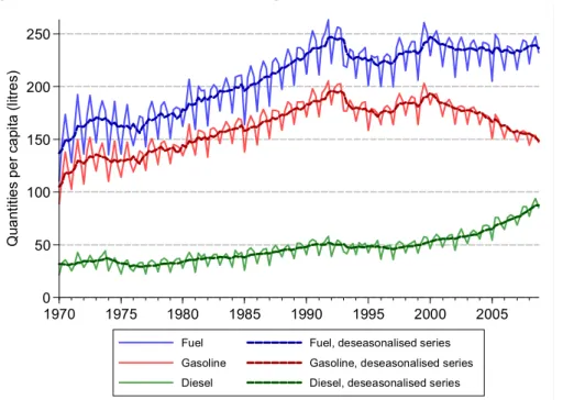
Figure 1 shows the evolution of gasoline, diesel, and fuel consumptions. The original series display substantial seasonal variations, and we deseasonalise the data before the analysis (thick lines in Figure 1).3 Quantities grew regularly until the beginning of
the 1990’s. Since 2000, gasoline consumption is however clearly decreasing, while diesel consumption is on the rise. Compared to other European countries (cf. EEA, 2012), the share of diesel in total fuel consumption is still relatively weak in Switzerland, as it only represents about one-third of the total amount of transport fuels.
3 We used the command ESMOOTH in the software RATS to deseasonalise the series. An alternative
strategy to analyse series showing seasonality would be to keep the raw data and introduce seasonal dummies. This does not alter our results significantly (available upon request). Except the deseasonalisation, all empirical analyses have been conducted in Stata.
Figure 1: Consumption of fuel, gasoline, and diesel, 1970-2008
Note: Fuel quantities correspond to the sum of gasoline and diesel quantities.
Several types of gasoline were delivered in Switzerland over the period 1970-2008.4
To analyse gasoline consumption over the whole period, we aggregate the different types in a single series, and we define gasoline price (PG) as the following weighted
average:
PG=
QU · PU + QL ∙ PR + PS2
QU + QL (3)
where QU (PU) is the quantity (price) of unleaded gasoline,5 and QL is the quantity of
leaded gasoline, which is either “regular” gasoline with price PR or “super” gasoline
4 “Regular” leaded gasoline was available in Switzerland until December 1984. Between October 1977
and December 1999, a more expensive type of leaded gasoline, called “super”, was also available. Unleaded gasoline was introduced in January 1985. The standard type of unleaded gasoline has 95 research octane number (RON). Since May 1993, 98 RON is also available as a more expensive option.
5 The price of unleaded gasoline (PU) is approximated by the price of 95 RON alone, since we do not
have separate data series for the quantities of 95 RON and 98 RON, but consumption of 98 RON is known to be much smaller. We do not have separate data for “regular” and “super” leaded gasoline quantities either, but because none of these two types of leaded gasoline are available over the entire observation period, we must consider both to define a complete price series. Over the period when both gasoline types are in the market (1977-1984), we use the unweighted average of their prices (PR and PS) as a proxy for the price of leaded gasoline. The price difference between “regular”
and “super” is anyway very small; it amounts to 3 cents of CHF per litre in average over 1977-1984.
0 50 100 150 200 250 Q uan titi es per c a pi ta ( lit re s) 1970 1975 1980 1985 1990 1995 2000 2005
Fuel Fuel, deseasonalised series Gasoline Gasoline, deseasonalised series Diesel Diesel, deseasonalised series
with price PS. This price is then deflated using the consumer price index (CPI) in
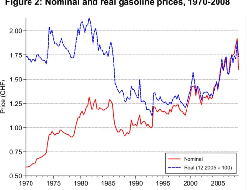
December 2005 CHF.6 Figure 2 displays the evolution of nominal and real gasoline
prices since 1970. Over the observation period, the mean real gasoline price was CHF 1.6 per litre, with a maximum at 2.1 (1981Q3) and a minimum at 1.1 (1993Q1). We point out the relatively high prices during the two oil shocks of 1973 and 1980, and the sharp increase since 2005, with a peak in summer 2008. It is also worth of notice that the 2008 real prices remained lower than those in 1973 and 1980.
Diesel prices are collected since 1993 only and nothing more than a production price index exists over the whole period 1970-2008. It is thus not possible to estimate a separate demand for diesel alone. Moreover, correlation between real gasoline prices and values of the diesel real price index is almost perfect (0.96), which prevents us from using both prices in the same regression. When estimating a total fuel demand, i.e. the sum of gasoline and diesel, we include gasoline prices only and leave aside all measures of diesel prices.
We also consider gasoline prices in foreign countries. This allows accounting for the “tank tourism” phenomena, which is relatively important in Switzerland (Banfi et al., 2005). We consider prices in the border regions of Germany, France, Italy, and Austria. These foreign prices are converted to Swiss francs using the contemporaneous exchange rates and then deflated using the Swiss CPI.7 We aggregate border prices
in a single variable by taking the average price, weighted by the kilometres of border with the neighbour countries.8 Gasoline prices in the foreign border regions are
6 In December 2005, CHF1 = US$0.77 = €0.65.
7 Before January 2002, different national currencies (DEM, FRF, ITL, and ATS) were used. Since
January 2002, all Switzerland’s neighbours use the Euro.
8 Results are quantitatively similar if we define foreign gasoline price as a simple (non-weighted)
generally higher than in Switzerland. Over the observation period, the mean foreign price was CHF 1.9 per litre of gasoline.
Figure 2: Nominal and real gasoline prices, 1970-2008
Following the existing literature, we use GDP per capita as a proxy for income. Of course, in the context of a demand function, it would have been preferable to use disposable income, but this variable is available since 1990 only.
In the long run, we expect gasoline and fuel demands to depend on the number of vehicles. Records for the total stock of vehicles (including trucks and motorbikes) are available, as well as for the vehicles stocks by fuel type (gasoline, diesel, electric, and others). We divide vehicles stocks by the number of individuals aged 20-76 years old, which seems a legitimate approximation for the number of drivers.9 The number of
vehicles per 1000 drivers was about 722 in average over the period, with a maximal
9 Schmalensee & Stoker (1999) highlight that, in the context of gasoline consumption, it is more
relevant to consider the number of car drivers as a determinant instead of total population, because it prevents demographic effects. Notably, using the former heavily reduces estimates of income elasticity. Because we do not observe the number of drivers directly, we follow Pock (2010) by considering individuals in a reasonable age range to approximate the number of car drivers.
0.50 0.75 1.00 1.25 1.50 1.75 2.00 Pri ce (C H F ) 1970 1975 1980 1985 1990 1995 2000 2005 Nominal Real (12.2005 = 100)
value of 928. The number of gasoline-powered passenger cars per 1000 drivers was on average 553, with a maximum of 653. Pock (2010) shows that using total stock of vehicles in the estimation of gasoline demand leads to an overestimation of the price, income and vehicles stock elasticities. Therefore, we use the stock of gasoline-powered passenger cars per driver in the gasoline demand, while we include the total stock of vehicles per driver in the estimation of fuel demand.
4. Results
We consider two demand equations: one for gasoline and another for total fuel (gasoline and diesel together). For both demands, we use the following long run relationship:
lnQt = β01 + β02I + β1lnPt + β2lnYt + β3lnVt + β4lnPFt + β5t. + zt, t = 1, ..., n. (4)
where Qt is gasoline (or fuel) consumption per capita in quarter t, Pt is real gasoline
price, Yt is GDP per capita, Vt is the stock of gasoline-powered passenger cars (or of
motor vehicles) per driver, PFt is real gasoline price in the foreign border areas, and t
is a linear trend, normalised from 0 (for t = 0) to 1 (for t = n), that captures technical progress.
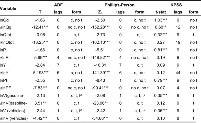
All the variables included in (4) were found to be stationary in first difference on the basis of the tests proposed by Dickey and Fuller (1979), Phillips and Perron (1988), and Kwiatkowski et al. (1992). The stationarity tests are available in Appendix.
It is a dummy variable included in (4) to account for potential breaks in the long run relationships, following the procedure by Gregory & Hansen (1996a, b):
It=
0, if t ≤ [n] 1, if t> [n]
where the unknown parameter є (0, 1) denotes the timing of the break point (relative to the observation period) and [·] denotes integer part. Our estimations show that there is a level shift (change in the constant) in both fuel and gasoline demands in the last quarter of 1990. We also tested for regime shifts (changes in both the constant and the slopes), but the results are inconclusive.
The estimation of (4) over the entire period 1970Q1-2008Q4 yields much larger residuals for the first 6 observations (1970Q1-1971Q2) than for later periods. This may indicate a first break point in 1971. Unfortunately, we lack observations prior to 1970 to rigorously test for it.10 For this reason, we discard the first 6 quarters and perform
our analysis over the reduced period 1971Q3-2008Q4.
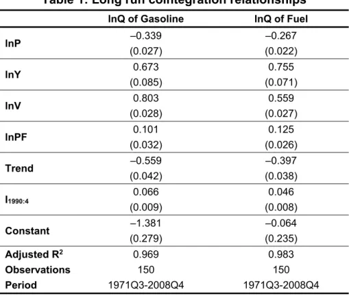
Table 1 reports the estimations for the gasoline and fuel cointegration relationships (equation 4). The estimated coefficients correspond to long run elasticities. As expected, the price elasticity of gasoline demand is relatively low in Switzerland (-0.34), even in the long run. The price elasticity of fuel demand is lower in absolute value (-0.27) than those for gasoline. An explanation is that substitution possibilities for gasoline are higher (e.g. switch to diesel) than for total fuel, which already includes diesel. Similar estimates of price elasticities were found for countries like the USA, Canada and Australia (see Section 1). As mentioned by Brons et al. (2008), in those countries and in Switzerland, consumers could be less sensitive to price because their income is relatively high and fuel prices relatively low. Our estimates are remarkably close to those of other studies about gasoline demand in Switzerland. Although using
10 Gregory & Hansen (1996a, b) indicate that at least 15% of the observations are required on each
side of the break point to permit the computation of all the necessary statistics. In our case, it means we can test for shifts over the period 1975Q5-2002Q4 only.
Interestingly, Wasserfallen & Güntensperger (1988), who analyse annual Swiss data over the period 1962-1985, find a break in the price coefficient between 1973 and 1974. However, they contend this may be due to a low variability in gasoline prices before 1973, which makes it difficult to identify the true parameter in the data.
a completely different methodology based on stated preferences, Erath & Axhausen (2010) report an identical value of -0.34 for the price elasticity of gasoline demand. Banfi et al. (2010), focusing on “tank tourism”, find that the price elasticity is about -1.5 in the Swiss border regions, but it falls to -0.3 farther than 30 kilometres away from the border.
Table 1: Long run cointegration relationships
lnQ of Gasoline lnQ of Fuel lnP –0.339 –0.267 (0.027) (0.022) lnY 0.673 0.755 (0.085) (0.071) lnV 0.803 0.559 (0.028) (0.027) lnPF 0.101 0.125 (0.032) (0.026) Trend –0.559 –0.397 (0.042) (0.038) I1990:4 0.066 0.046 (0.009) (0.008) Constant –1.381 –0.064 (0.279) (0.235) Adjusted R2 0.969 0.983 Observations 150 150 Period 1971Q3-2008Q4 1971Q3-2008Q4
Note: standard errors in parenthesis.
Income elasticity is +0.67 for gasoline and +0.76 for fuel. In accordance with the literature, gasoline and fuel are found to be first necessity goods: an increase in income implies an increase in quantity less than proportional.
We obtain that an increase by 1% of the gasoline-powered cars stock per driver increases gasoline consumption by 0.8%, while an increase by 1% of the vehicles stock per driver increases fuel consumption by about 0.6%. The greater efficiency of diesel-powered vehicles might explain why vehicle elasticity of fuel consumption is lower than car elasticity of gasoline consumption. The fact that these two elasticities
are smaller than unity probably stems from increasing technical efficiency: new vehicles being more efficient than older cohorts, consumption increases slower than the stock of vehicles.
The estimated elasticity with respect to the prices in the foreign border regions is +0.1 for both gasoline and fuel demands. An increase by 1% of real gasoline prices in the foreign border areas thus induces gasoline and fuel consumptions in Switzerland to rise by 0.1%. This elasticity seems relatively weak. However, we emphasize that the impact is measured with respect to gasoline or fuel consumption over the whole Swiss territory. In fact, our result is perfectly consistent with the price elasticity of 1.2 measured by Banfi et al. (2010) when limited to Swiss border regions.11
The trend coefficient is negative in both demands, which can be explained by an increase in gasoline and fuel efficiency use. The trend values are normalised between 0 and 1, so that its coefficient can be interpreted as the percentage variation in consumption between the first and the last periods under observation, all other factors remaining constant. If no factor considered in the demand equations had changed between 1971 and 2008, gasoline consumption would have decreased by 43% and fuel consumption by 33%.12
The dummy variable I1990:4 accounts for the structural break identified in the
cointegration relationships between 1990Q4 and 1991Q1. It takes the value 0 until the 4th quarter 1990 and the value 1 since the 1st quarter 1991. The coefficients associated
to this variable are positive. Since 1991, demand for gasoline has increased by 6.8%
11 Given that tank tourism accounts for 5% to 10% of overall gasoline consumption in Switzerland over
the period 2001-2008 considered by Banfi et al. (2010), a price elasticity of 1.2 in border regions roughly corresponds to price elasticity between 0.06 and 0.12 in the entire country.
12 Because gasoline and fuel are taken in logarithms, the effect of a change from 0 to 1 in the trend has
and demand for fuel by 4.7%, all other things being equal. We emphasize that the breaks in cointegration relationships are found by statistical investigation only, and they do not necessarily coincide with any precise economic event. Some caution is moreover needed in the interpretation of the break points, especially when samples are relatively small (see Hassler, 2003; Kim et al. 2004; Tsay & Chung, 2000). It is however not surprising to find a shift at the end of 1990 if we go back to Figure 1, where we observe a clear change in the evolution of gasoline and fuel consumptions.
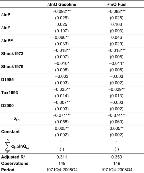
To investigate the short run dynamics, we estimate the following error correction model:
∆lnQt = α0 + α1∆lnPt + α2∆lnYt + α3∆lnPFt + α4Shock1973 + α5Shock1979 +
α6D1985 + α7Tax1993 + α8D2000 + ∑ α9i∆lnQt–i + γzt-1 + εt, (5) where Qt, Pt, Yt, and PFt are defined as before. They are taken in first-differences
(indicated by ) to make them stationary. Shock1973 and Shock1979 are dummy variables accounting for the impact of the first and second oil shocks. Shock1973 takes the value 1 from 1973Q4 to 1974Q3, while Shock1979 is 1 from 1978Q4 to 1979Q4. Those periods have been chosen by inspection of the gasoline price variations in Switzerland (see Figure 2). The dummy variable D1985 takes the value 1 since 1985Q1 and accounts for the introduction of unleaded gasoline in the Swiss market. The dummy variable D2000 takes the value 1 since 2000Q1 and accounts for the abolition of leaded gasoline. The dummy Tax1993 takes the value 1 for 1993Q2 only. This variable accounts for a possible impact of the mineral oil tax increase of about 25 cents per gross 100 Kg introduced in March 1993. zt-1 represents the error correction term and is given by the lagged residuals of the long run cointegration relationship (4). To eliminate autocorrelation, it was necessary to include five lags of the endogenous
variable (∆lnQt-i = lnQt-i – lnQt-i-1) in the explanatory variables. Relation (5) does not
include the vehicles stock, since it can be considered as fixed in the short run.13
We tried various short run models, also including additional explicative variables such as meteorological variables (e.g. rain, temperature) or prices indexes for various goods, but they were not statistically significant. Table 2 reports the results of our preferred estimation.
In the short run, price elasticity is estimated at -0.09 for gasoline demand and -0.08 for fuel demand. As expected theoretically, demands are more inelastic in the short than in the long run. Price elasticities are very weak, since an increase of the price by 1% would decrease demand by less than 0.1%, all other things being equal. Such results are comparable to the value of -0.06 obtained in Carlevaro et al. (1992).
GDP per capita has no statistically significant impact in the short run. This was not unexpected, since consumers need time before reacting to income variations. In the short run, habits dictate the consumption path. The results also show that prices in the foreign border regions have a weak impact on short run gasoline demand and no significant impact on short run fuel consumption. An increase by 1% of the gasoline price in the foreign border regions increases the Swiss gasoline demand by 0.07%. Once again, it is not surprising that this elasticity is lower than in the long run. Carlevaro et al. (1992) also find that Swiss gasoline demand reacts weakly to price differentials between Switzerland and Italy (average elasticity of -0.07).
The 1993 increase of the mineral oil tax decreased gasoline demand by about 3.5% and fuel demand by about 3%. We emphasize that this impact comes in addition to
13 Moreover, we cannot use vehicles stocks in differences due to the design of these data. Vehicles
stocks are collected only once a year and we constructed quarterly values by linear interpolation. It would be meaningless to differentiate such a variable, since its growth rate is by definition constant within a year.
that caused by the price increase arising from the tax. An increase in the mineral oil tax thus has two distinct impacts, both of which decrease demand: first, the price increase itself, then, an additional reaction by consumers, who know that this price increase is not a natural variation resulting from market forces. The fact that consumers’ reaction depends on the source of price variation is a consistent finding in the literature. Davis & Kilian (2011) find that tax elasticity is much larger than price elasticity. Ghalwash (2007) also obtains differentiated effects, but his results on different types of goods are somewhat ambiguous. Li et al. (2012) find a much larger effect of tax increase and point to an interesting explanation: because gasoline tax changes are subject to public debates and attract a great deal of attention from the media, this could contribute to reinforce consumers’ reaction. Scott (2012) finally finds consumers to be twice as responsive to tax-driven price changes as to market-driven price changes.
The two oil shocks have decreased fuel and gasoline demands: -1.8% in 1973 and -1.0/1.1% in 1979. In this case too, the short run impact has to be added to the effects of price rises that occurred during the oil shocks. Like tax increases, oil crises receive substantial media coverage. This gives credit to Li et al.’s (2012) argument that factors receiving high media coverage magnify consumers’ reaction.
The abolition of leaded gasoline, represented by D2000, had a statistically significant negative impact on gasoline demand, but not on fuel. If fuel demand has not changed while gasoline demand decreased since 2000, this might indicate substitution effects between gasoline and diesel. When leaded gasoline was abolished, a number of drivers who possessed a leaded gasoline-powered car probably switched to a diesel-powered car, instead of buying a new (unleaded) gasoline-diesel-powered car.
The coefficients for the error correction terms are -0.27 for gasoline demand and -0.37 for fuel demand, which implies that 27% of long run disequilibrium in gasoline demand and 37% of disequilibrium in fuel demand are absorbed in one quarter. Adjustment speed is relatively high, as more than 80% of deviations from long run equilibrium are absorbed after 1.5 years (gasoline) and 1 year (fuel).14
Table 2: Short run relationships
∆lnQ Gasoline ∆lnQ Fuel ∆lnP –0.092*** –0.082*** (0.028) (0.025) ∆lnY 0.025 0.103 (0.107) (0.093) ∆lnPF 0.066** 0.046 (0.033) (0.029) Shock1973 –0.018** –0.018*** (0.007) (0.006) Shock1979 –0.010* –0.011* (0.006) (0.006) D1985 –0.003 –0.003 (0.003) (0.002) Tax1993 –0.035** –0.029** (0.014) (0.013) D2000 –0.007** –0.003 (0.003) (0.002) zt-1 –0.271*** –0.374*** (0.058) (0.060) Constant 0.005** 0.005** (0.002) (0.002) α9i∆lnQt-i 5 i=1 · · (·) (·) Adjusted R2 0.311 0.350 Observations 149 149 Period 1971Q4-2008Q4 1971Q4-2008Q4
Notes: standard errors in parenthesis; ***, **, *: statistically significant at 1%, 5% and 10%.
14 We checked the robustness of the results using annual data. The results (available on request) are
5. Summary and conclusions
In this paper, we analyse demands for gasoline and for fuel (gasoline and diesel together) in Switzerland. Using quarterly data from 1970 to 2008, we are able to investigate a larger number of explicative variables than most studies of the literature. Using Engle and Granger’s (1987) cointegration approach, we establish a short and a long run relationship.
The main results are the following. In Switzerland, demands for gasoline and for fuel are weakly sensitive: price elasticities are about -0.3 in the long run. In the short run, demand is very inelastic: estimates of price elasticities are -0.09 for gasoline and -0.08 for fuel.
Gasoline and fuel demands are sensitive to price variations in foreign countries. In the long run, an increase by 1% of gasoline prices in foreign border regions induces gasoline and fuel demands in Switzerland to rise by about 0.1%. Those results refer to the whole Swiss market, which does not mean that foreign prices do not have a much stronger impact in regions close to borders.
Our results also show that the 1973 and 1979 oil shocks as well as the 1993 mineral oil tax increase possess an additional impact on gasoline and fuel demands, on top of their direct impact due to price increase. For instance, leaving aside the price rise it provoked, the increase in mineral oil tax per se decreased fuel demand by about 3% and gasoline demand by about 3.5%. In spite of this additional short run impact, our results show that the price increase should be substantial in order to reduce fuel consumption and curb CO2 emissions. Moreover, substantial fiscal revenues could be
collected through taxes on gasoline. Significant distributive impacts might however emerge due to the diversity of the Swiss territory (urban, rural, mountainous regions).
References
Akinboade, O.A., Ziramba, E. & Kumo, W.L. (2008): “The Demand for Gasoline in South Africa: An Empirical Analysis using Co-integration Techniques”, Energy Economics, 30(6): 3222–3229. Alves, D.C.O. & Bueno R.D. (2003): “Short-run, Long-run and Cross Elasticities of Gasoline Demand in
Brazil”, Energy Economics, 25(2): 191–199.
Ayat, L. & Burridge, P. (2000): “Unit Root Tests in the Presence of Uncertainty about the Non-stochastic Trend”, Journal of Econometrics, 95(1): 71–96.
Banfi, S., Filippini, M., Heimsch, F., Keller, M. & Wüthrich, P. (2010): Tanktourismus. Bern: Swiss Federal Office of Energy, BFE-Projektnummer: 102749.
Banfi, S., Filippini, M. & Hunt, L. (2005): “Fuel Tourism in Border Region: The Case of Switzerland”,
Energy Economics, 27(5): 689–707.
Bentzen, J. (1994): ‘‘An Empirical Analysis of Gasoline Demand in Denmark using Cointegration Techniques’’, Energy Economics, 16(2): 139–143.
Blum, U., Foos, G., & Guadry, M. (1988): ‘‘Aggregate Time Series Gasoline Demand Models: Review of the Literature and New Evidence for West Germany’’, Transportation Research Part A: General,
22(2): 75–88.
Brons, M., Nijkamp, P., Pels, E., & Rietveld, P. (2008): “A Meta-Analysis of the Price Elasticity of Gasoline Demand. A SUR Approach”, Energy Economics, 30(5): 2105–2122.
Carlevaro, F., Bertholet, J.–L., Chaze, J.–P. & Taffé, P. (1992): “Engineering-Econometric Modeling of Energy Demand”, Journal of Energy Engineering, 118(2): 109–121.
Crôtte, A., Noland, R.B. & Graham, D.J. (2009): “An Analysis of Gasoline Demand Elasticities at the National and Local Levels in Mexico”, Energy Policy, 38(8): 4445–4456.
Dahl, C. & Sterner, T. (1991): “Analysing Gasoline Demand Elasticities: A Survey”, Energy Economics,
13(3): 203–210.
Davis, L.W. & Kilian, L. (2011): “Estimating the Effect of a Gasoline Tax on Carbon Emissions”, Journal
of Applied Econometrics, 26(7): 1187–1214.
Dickey, D.A. & Fuller, W.A. (1979): “Distribution of the Estimators for Autoregressive Time Series with a Unit Root”, Journal of the American Statistical Association, 74(366): 427–431.
Eltony, M.N. & Al-Mutairi, N.H. (1995): “Demand for Gasoline in Kuwait: An Empirical Analysis using Cointegration Techniques”, Energy Economics, 17(3): 249–253.
Eltony, M. (1993): ‘‘Transport Gasoline Demand in Canada’’ Journal of Transport Economics and Policy,
27(2): 193–208.
Engle, R.F & Granger, W.J. (1987): “Co-integration and Error Correction: Representation, Estimation, and Testing”, Econometrica, 55(2): 251–276.
Erath, A. & Axhausen, K.W. (2010): “Long Term Fuel Price Elasticity: Effects on Mobility Tool Ownership and Residential Location Choice.” Bern: Swiss Federal Office of Energy, BFE-Projektnummer: 102940.
European Energy Agency (EEA) (2012): Dieselisation in the EEA, http://www.eea.europa.eu/.
FOEN (2013): Réalisation des objectifs de réduction du Protocole de Kyoto et de la loi sur le CO2. Bern:
Federal Office for the Environment.
Ghalwash, T. (2007): “Energy Taxes as a Signaling Device: An Empirical Analysis of Consumer Preferences”, Energy Policy, 35(1): 29-38.
Graham D.J. & Glaister, S. (2002): “The Demand for Automobile Fuel. A Survey of Elasticities”, Journal
of Transport Economics and Policy, 36(1): 1–25.
Gregory, A.W., & Hansen, B.E. (1996a): “Residual-based Test for Cointegration in Models with Regime Shifts", Journal of Econometrics, 70(1): 99–126.
Gregory, A.W., & Hansen, B.E. (1996b): “Tests for Cointegration in Models with Regime and Trend Shifts”, Oxford Bulletin of Economics and Statistics, 58(3): 555–559.
Halvorsen R. & Palmquist, R. (1980): “The Interpretation of Dummy Variables in Semilogarithmic Equations”, American Economic Review, 70(3): 474–475.
Hassler, U. (2003): “Nonsense Regressions Due to Neglected Time-varying Means”, Statistical Papers,
Hensher, D.A., Smith, N.C., Milthorpe, F.W. & Barnard, P.O. (1992): Dimensions of Automobile
Demand: A Longitudinal Study of Household Automobile Ownership and Use, North Holland,
Amsterdam.
Kim, T., Lee, Y., Newbold, P. (2004): “Spurious Regressions with Stationary Processes around Linear Trends”, Economics Letters, 83(2): 257-262.
Kwiatkowski, D., Phillips, P.C.B., Schmidt, P., & Shin, Y. (1992): “Testing the null hypothesis of Stationarity against the Alternative of a Unit Root: How Sure are we that Economic Time Series have a Unit Root?” Journal of Econometrics, 54(1-3): 159–178.
Li, S., Linn, J. & Muehlegger, E. (2012): “Gasoline Taxes and Consumer Behavior”, Working Paper Series rwp12-006, Harvard University, John F. Kennedy School of Government.
Lipow, G.W. (2008): “Price–Elasticity of Energy Demand: A Bibliography”, Carbon Tax Center (www.carbontax.org).
Maddala, G.S. & Kim, I.-M. (1998): Unit Roots, Cointegration, and Structural Change, Cambridge University Press, Cambridge.
Nicol, C.J. (2003): “Elasticities of Demand for Gasoline in Canada and the United States” Energy
Economics, 25(2): 201–214.
Phillips, P.C. & Perron, P. (1988): “Testing for a Unit Root in Time Series Regression. Biometrika, 75(2): 335–346.
Pock, M. (2010): “Gasoline Demand in Europe: New Insights”, Energy Economics, 32(1): 54–62. Polemis M.L. (2006): “Empirical Assessment of the Determinants of Road Energy Demand in Greece”,
Energy Economics, 28(3): 385–403.
Rao, B.B. & Rao, G. (2009): “Cointegration and the Demand for Gasoline”, Energy Policy, 37(10): 3978– 3983.
Rouwendal, J. (1996): ‘‘An Economic Analysis of Fuel Use per Kilometre by Private Cars’’, Journal of
Transport Economics and Policy, 30(1): 3–14.
Samini, R. (1995): “Road Transport Energy Demand in Australia”, Energy economics, 17(4): 329–339. Schleiniger, R. (1995): “The Demand for Gasoline in Switzerland – in the Short and in the Long Run”,
Discussion paper 9053, Institute for Empirical Research in Economics, University of Zurich.
Schmalensee, R. & Stoker, T.M. (1999): “Household Gasoline Demand in the United States”,
Econometrica, 67(3): 412–418.
Sentenac-Chemin, E. (2012): “Is the Price Effect on Fuel Consumption Symmetric? Some Evidence from an Empirical Study”, Energy Policy, 41: 59–65.
Scott, K.R. (2012): “Rational Habits in Gasoline Demand”, Energy Economics, forthcoming.
Tsay, W. & Chung, C. (2000): “The Spurious Regression of Fractionally Integrated Processes”, Journal
of Econometrics, 96(1): 155–182.
Wasserfallen, W. & Güntensperger, H. (1988): “Gasoline Consumption and the Stock of Motor Vehicles – An Empirical Analysis for the Swiss Economy”, Energy Economics, 10(4): 276–282.
Appendix
Table A.1: Stationarity tests
Variable ADF Phillips-Perron KPSS
T lags form Z lags form t-stat lags form
lnQg -1.66 0 c, no t -2.50 0 c, no t 1.03*** 9 no t ∆lnQg -12.41*** 0 no c, no t -152.28*** 0 no c, no t 0.60** 12 no t lnQtot -0.96 0 c, t -2.73 0 c, t 0.32*** 9 t ∆lnQtot -13.25*** 0 c, no t -162.10*** 0 c, no t 0.27 19 no t lnP -1.66 0 c, no t -5.51 0 c, no t 0.81*** 9 no t ∆lnP -5.99*** 4 no c, no t -148.82*** 4 no c, no t 0.19 9 no t lnY -2.84 7 c, t -16.31 7 c, t 0.09 9 t ∆lnY -5.198*** 6 c, no t -141.39*** 6 c, no t 0.12 44 no t lnPF -2.55 1 c, no t -8.43 1 c, no t 0.79*** 9 no t ∆lnPF -7.83*** 0 no c, no t -99.41*** 0 no c, no t 0.07 4 no t lnV(gasoline- -2.13 1 c, t, t2 -2.08 1 c, t, t2 0.35*** 9 t ∆lnV(gasoline- 3.51** 0 c, t -23.96** 0 c, t 0.12 9 t lnV (vehicles) -2.44 1 c, t, t2 -2.42 1 c, t, t2 0.36*** 9 t ∆lnV (vehicles) -4.42*** 0 c, t -34.68*** 0 c, t 0.10 8 t
Notes: ***/**/* denotes a t-ratio significant at the 1/5/10% level.
For ADF and Phillips-Perron tests, the number of lags (with a maximum of 8) was selected on the basis of the AIC, BIC, and HQIC.
For KPSS test, the number of lags was selected by automatic bandwidth selection, and autocovariances weighted by Bartlett kernel.
c = constant, t = linear trend, t2 = quadratic trend.
Critical values for unit root test with quadratic trend are provided by Ayat & Burridge (2000, Appendix B).