HAL Id: hal-00765276
https://hal.inria.fr/hal-00765276
Submitted on 14 Dec 2012
HAL is a multi-disciplinary open access
archive for the deposit and dissemination of
sci-entific research documents, whether they are
pub-lished or not. The documents may come from
teaching and research institutions in France or
abroad, or from public or private research centers.
L’archive ouverte pluridisciplinaire HAL, est
destinée au dépôt et à la diffusion de documents
scientifiques de niveau recherche, publiés ou non,
émanant des établissements d’enseignement et de
recherche français ou étrangers, des laboratoires
publics ou privés.
Hermitian Interpolation Subject to Uncertainties
Jean-Antoine Désidéri, Manuel Bompard, Jacques Peter
To cite this version:
Jean-Antoine Désidéri, Manuel Bompard, Jacques Peter. Hermitian Interpolation Subject to
Uncer-tainties. Repin, S. and Tiihonen, T. and Tuovinen, T. Numerical Methods for Differential Equations,
Optimization, and Technological Problems, 27, Springer Dordrecht, pp.193-218, 2013, Computational
Methods in Applied Sciences, 978-94-007-5288-7. �10.1007/978-94-007-5288-7�. �hal-00765276�
Jean-Antoine D´esid´eri, Manuel Bompard, and Jacques Peter
Abstract This contribution is a sequel of the report [1]. In PDE-constrained global
optimization (e.g., [3]), iterative algorithms are commonly efficiently accelerated by techniques relying on approximate evaluations of the functional to be minimized by an economical but lower-fidelity model (“meta-model”), in a so-called “Design of Experiment” (DoE) [6]. Various types of meta-models exist (interpolation polyno-mials, neural networks, Kriging models, etc.). Such meta-models are constructed by pre-calculation of a database of functional values by the costly high-fidelity model. In adjoint-based numerical methods, derivatives of the functional are also available at the same cost, although usually with poorer accuracy. Thus, a question arises: should the derivative information, available but known to be less accurate, be used to construct the meta-model or be ignored? As the first step to investigate this issue, we consider the case of the Hermitian interpolation of a function of a single variable, when the function values are known exactly, and the derivatives only approximately, assuming a uniform upper bound!on this approximation is known. The classical notion of best approximation is revisited in this context, and a criterion is intro-duced to define the best set of interpolation points. This set is identified by either analytical or numerical means. If n+ 1 is the number of interpolation points, it is advantageous to account for the derivative information when!≤!0, where!0 de-creases with n, and this is in favor of piecewise, low-degree Hermitian interpolants. In all our numerical tests, we have found that the distribution of Chebyshev points is always close to optimal, and provides bounded approximants with close-to-least sensitivity to the uncertainties.
Jean-Antoine D´esid´eri
INRIA, Centre de Sophia Antipolis - M´editerran´ee, BP 93, 2004 Route des Lucioles, F-06902 Sophia Antipolis cedex, France, e-mail: [email protected]
Manuel Bompard, Jacques Peter
ONERA/DSNA, BP 72, 29, Avenue de La Division Leclerc, F-91322 Chˆatillon cedex, France, e-mail: [email protected], [email protected]
1 Introduction: the Classical Notion of Best Approximation
In this section, we review certain classical notions on polynomial interpolation, in particular the concept of “best approximation” or “Chebyshev economization”. The literature contains numerous elementary and advanced texts on this fundamental issue, and we refer to [2, 4, 5].Let n be an integer and x0, x1, ..., xn be n+ 1 distinct points of the normalized
interval [-1,1]. Let"(x) be the following polynomial of degree n + 1:
"(x) =
n
#
i=0
(x − xi) (1)
and consider the following n+ 1 polynomials of degree n: Li(x) = n
#
j=0 j#=i x− xj xi− xj (i = 0, 1, ..., n) . (2) Clearly ∀i, j ∈ {0,1,...,n} : Li(xj) =$i, j, (3)where$ stands for Kr¨onecker’s symbol. Application of L’Hospital’s rule yields the following compact formula:
Li(x) = "(x)
"′(xi)(x − xi). (4) Let f :[−1,1] → R be a smooth function of the real variable x. The polynomial
Pn(x) = n
%
i=0
f(xi) Li(x) (5)
is of degree at most equal to n, and it clearly satisfies the following interpolation conditions:
∀i ∈ {0,1,...,n} : Pn(xi) = f (xi) . (6)
One such interpolant is unique among all polynomials of degree≤ n. Thus, Pn(x) is
the Lagrange interpolation polynomial of f at the points{xi}0≤i≤n.
It is well known that if f ∈ Cn+1([−1,1]), for any given x ∈ [a,b], the interpola-tion error is given by
en(x) = f (x) − Pn(x) =
f(n+1)(&)
(n + 1)! "(x) (7)
for some&∈ [−1,1].
Proof. Let x∈ [−1,1] be given. If x = xifor some i, the result is trivially satisfied.
' =en(x)
"(x) so that
f(x) = Pn(x) +' "(x)
and define the function
((t) = f (t) − Pn(t) −' "(t) t ∈ [−1,1].
The function((t) is of class Cn+1([−1,1]) and it admits a nonempty set of roots in the interval[−1,1] that includes X = {x0, x1, ..., xn, x}. The n + 2 elements of X
are distinct and can be arranged as the elements of a strictly increasing sequence {x0
i}0≤i≤n+1whose precise definition depends on the position of x w.r.t. the interpo-lation points{xi}0≤i≤n. By application of Rolle’s theorem to((t) =((0)(t) over the subinterval[x0
i, x0i+1], i = 0, 1, ..., n, it follows that(′(t) admits a root x1i in the open
interval]x0
i, x0i+1[, and this, for each i. In this way we identify a strictly-increasing sequence of n+ 1 roots of(′(t), {x1
i}0≤i≤n. Then Rolle’s theorem can be applied in a similar way, this time to(′(t), and so on to the successive derivatives of((t). We conclude that in general ((k)(t) admits at least n + 2 − k distinct roots in [-1,1],{xk
i}0≤i≤n+1−k, 0≤ k ≤ n + 1. In particular, for k = n + 1,((n+1)(t) admits at least one root, xn0+1, hereafter denoted& for simplicity. But since Pn(n+1)(&) = 0 and
"(n+1)(&) = (n + 1)!, one gets
'= f
(n+1)(&) (n + 1)! and the conclusion follows. !
Hence, if K= 1 (n + 1)!x∈[−1,1]max ! ! !f (n+1)(x)!! ! (8) we have ∀x ∈ [−1,1] : |en(x)| ≤ K |"(x)| . (9)
Therefore, a natural way to optimize the choice of interpolation points a priori, that is, independently of f , is to solve the following classical min-max problem:
min {xi}0≤i≤n xi∈[−1,1], ∀i
max
x∈[−1,1]|"(x)| . (10)
In view of this, the problem is to find among all polynomials"(x) whose highest-degree term is precisely xn+1, and that admit n+ 1 distinct roots in the interval [−1,1], an element, unique or not, that minimizes the sup-norm over [−1,1].
The solution of this problem is given by the n+ 1 roots of the Chebyshev polyno-mial of degree n+ 1. Before recalling the proof of this, let us establish some useful auxiliary results. Let k be an arbitrary integer and Tk(x) denote the Chebyshev
poly-nomial of degree k. Recall that for x∈ [−1,1]
Tk(x) = cos"k cos−1x# , k ∈ N, (11)
so that, for k≥ 1 and x ∈ [−1,1],
Tk+1(x) + Tk−1(x) = cos"k + 1)# + cos"k − 1)# = 2cos(k)) cos)= 2xTk(x),
(12) where one has let
x= cos), 0≤)≤". (13)
Thus, if the leading term in Tk(x) is say akxk, the following recursion applies:
ak+1= 2ak, k≥ 1, (14)
and, since a0= a1= 1, it follows that
ak= 2k−1, k≥ 1. (15)
Therefore, an admissible candidate solution for the min-max problem, (10), is the polynomial
"⋆(x) = 1
2nTn+1(x). (16)
It remains to establish that"⋆(x) is the best choice among all admissible polynomi-als, and its roots the best possible interpolation points. To arrive at this, we claim the following lemma:
Lemma 1. For all admissible polynomial q(x) one has
)"⋆) ≤ )q), (17)
where) ) is the sup-norm over [−1,1].
Proof. Assume otherwise that an admissible polynomial q(x) of a strictly smaller sup-norm over[−1,1] exists:
)q) < )"⋆). (18)
Let r(x) ="⋆(x) − q(x). Since the admissible polynomials"⋆(x) and q(x) have the same leading term, xn+1, the polynomial r(x) is of degree at most n. Let us examine the sign of this polynomial at the n+ 2 points
*i= cos
i"
n+ 1, i= 0, 1, ..., n + 1, (19)
at which"⋆(x) as well as T
n+1(x) achieve a local extremum. At such a point, |"⋆(* i)| = 1 2n =)" ⋆) > )q) = max x∈[−1,1]|q(x)| ≥ |q(*i)| (20)
and r(*i) is nonzero and has the sign of the strictly dominant term "⋆(*i) =
1
2nTn+1(*i) = (−1) i
2n . Therefore, r(x) admits at least n + 1 sign alternations and as
many distinct roots. But this is in contradiction with the degree of this polynomial. The contradiction is removed by rejecting the assumption made on)q). !
Consequently, in (10), the min-max is achieved by the roots of Tn+1(x):
x⋆
i = cos
(2i + 1)"
2(n + 1), i= 0, 1, ..., n, (21)
and the value of the min-max is 21n.
2 Best Hermitian Approximation
Now assume that the points{xi}0≤i≤nare used as a support to interpolate the func-tion values{yi= f (xi)}0≤i≤n, but also the derivatives{y′i= f′(xi)}0≤i≤n, that is a set of 2(n + 1) data. Thus, we anticipate that the polynomial of least degree com-plying with these interpolation conditions, say H2n+1(x), is of degree at most equal to 2n+ 1. One such polynomial is necessarily of the form
H2n+1(x) = Pn(x) +"(x) · Q(x), (22)
where the quotient Q(x) should be adjusted to comply with the interpolation condi-tions on the derivatives. These condicondi-tions are
y′i= H2n+1′ (xi) = Pn′(xi) +"i′· Q(xi), i= 0, 1, ..., n, (23) where "i′="′(xi) =
#
j=0 j#=i (xi− xj) #= 0, (24)and since"(xi) = 0. Thus Q(x) is solely constrained by the following n + 1
interpo-lation conditions: Qi= Q(xi) = y′i− Pn′(xi) "′ i , i= 0, 1, ..., n. (25)
Therefore, the solution of least degree is obtained when Q(x) is the Lagrange inter-polation polynomial associated with the above function values:
Q(x) =
n
%
i=0
QiLi(x). (26)
The corresponding solution is thus unique, and we will refer to it as the global Hermitian interpolant.
The interpolation error associated with the above global Hermitian interpolant
H2n+1(x) is given by the following result valid when f ∈ C2n+2([−1,1]):
∀x ∈ [−1,1], ∃*∈ [−1,1] : f (x) = H2n+1(x) +
f(2n+2)(*) (2n + 2)! "
2(x).
(27)
Proof. Let x∈ [−1,1] be given. If x = xifor some i, the result is trivially satisfied.
Otherwise,"(x) #= 0; then let
µ= f(x) − H2n+1(x) "2(x) so that f(x) = H2n+1(x) +µ"2(x) . Let +(t) = f (t) − H2n+1(t) −µ"2(t), t∈ [−1,1].
The function+(t) is of class C2n+2([−1,1]), and similarly to the former function ((t), it admits a nonempty set of roots in the interval [−1,1] that includes X = {x0, x1, ..., xn, x} = {x0i}0≤i≤n+1. Hence, Rolle’s theorem implies that in the open interval]xi, xi+1[, 0 ≤ i ≤ n, a root x′iof+′(t) exists. But the interpolation points, at
which the derivative also is fitted, are themselves n+ 1 other distinct roots of+′(t). Thus we get a total of at least 2n+ 2 roots for+′(t), and by induction, 2n + 1 for
+′′(t), and so on, and finally one, say*, for+(2n+2)(t). Now, since H(2n+2) 2n+1 (*) = 0 because the interpolant is of degree 2n+ 1 at most, and since ("2(t))(2n+2)(t) = (2n + 2)!, one gets
0= f(2n+2)(*) − 0 −µ(2n + 2)! which yields the final result. !
As a consequence of (27), the formulation of the best approximation problem for the global Hermitian interpolant is as follows:
min {xi}0≤i≤n xi∈[−1,1], ∀i max x∈[−1,1]" 2(x). (28)
But, if we define the following functions of Rn+1→ R: P(x0, x1, ..., xn) = max x∈[−1,1]" 2(x), p(x0, x1, ..., xn) = max x∈[−1,1]|"(x)|, (29) it is obvious that ∀x0, x1, ..., xn : P(x0, x1, ..., xn) = p2(x0, x1, ..., xn). (30)
Hence the functions P and p achieve their minimums for the same sequence of interpolation points, and
min {xi}0≤i≤n xi∈[−1,1], ∀i P(x0, x1, ..., xn) = {xmin i}0≤i≤n xi∈[−1,1], ∀i p(x0, x1, ..., xn) 2 = 1 4n. (31)
Therefore the best Hermitian interpolation is achieved for the same set of interpola-tion points as the best Lagrangian interpolainterpola-tion, that is, the roots,{x⋆
i}0≤i≤nof (21), of the Chebyshev polynomial Tn+1(x).
3 Best Inexact Hermitian Approximation
In PDE-constrained global optimization [3], it is often useful to model the functional criterion to be optimized by a function f(x) of the design variable x ∈ Rn, whose
values are computed through the discrete numerical integration of a PDE, and the derivative f′(x), or gradient vector, by means of an adjoint equation. A database of function values and derivatives is compiled by Design of Experiment, and the sur-rogate model, or meta-model is constructed from it. This meta-model is then used in some way in the numerical optimization algorithm with the objective of improv-ing computational efficiency (see, for example, [3]). The success of such a strategy depends on the accuracy of the meta-model f(x) to represent the dependency on x of the actual functional criterion. If all the data were exact, and properly used, the accuracy would undoubtedly improve by the addition of the derivative information. However, in practice, since the PDE is solved discretely, the derivatives are almost inevitably computed with inferior accuracy. Therefore it is not clear that accounting for the derivatives is definitely advantageous if the corresponding accuracy of the data is poor. Should special precautions be taken to guarantee it?
In order to initiate a preliminary analysis of this problem, we examine the simple one-dimensional situation of a function f(x), when x is scalar (x ∈ R), and con-sider the case of a Hermitian interpolation meta-model based on inexact informa-tion. Specifically, we assume that the function values{yi}0≤i≤nare known, whereas only approximations{ y′
i}0≤i≤nof the derivatives{y′i}0≤i≤nare available, and we let: $y′i= y′i− y′i:=!i, i= 0, 1, ..., n. (32)
Hence the computed interpolant is H2n+1(x) instead of H2n+1(x), and in view of the definitions (22)–(25), we have
$H2n+1(x) = H2n+1(x) − H2n+1(x) ="(x)$Q(x), $Q(x) = n
%
i=0 $QiLi(x), $Qi= $y′i "′ i = !i "′ i . (33)Now, suppose an upper bound!on the errors!i’s is known:
|!i| ≤!, 0≤ i ≤ n. (34)
The following questions arise:
1. What is the corresponding upper bound on maxx∈[−1,1]|$H2n+1(x)|?
2. Can we choose the sequence of interpolation points{xi}0≤i≤nto minimize this upper bound?
3. Is the known sequence of the Chebyshev points a good approximation of the optimum sequence for this new problem?
This article attempts to bring some answers to these questions. Presently, we try to identify how the interpolation points should be defined to minimize or reduce the effect on the meta-model accuracy of uncertainties on the derivatives only. It follows from (33) that $H2n+1(x) ="(x) n
%
i=0 !i "′ i Li(x) (35)which by virtue of (4) simplifies as follows:
$H2n+1(x) ="2(x) n
%
i=0 !i "′ i 2 (x − xi) . (36)Thus if (34) holds, we have
|$H2n+1(x)| ≤!,(x) (37) where ,(x) ="2(x) n
%
i=0 1 "′ i 2 |x − xi| . (38)These considerations have led us to analyze the min-max problem applied to the new criterion,(x) in place of"2(x). In summary, the solution of the min-max prob-lem associated with the criterion,(x) minimizes the effect of uncertainties in the derivatives on the identification of the global Hermitian interpolant. In the subse-quent sections, this solution is identified formally, or numerically, and compared with the Chebyshev distribution of points, which is optimal w.r.t. the interpolation error. Lastly, the corresponding interpolants are compared by numerical experiment.
4 Formal or Numerical Treatment of the Min-Max-
,
Problem
We wish to compare three particular relevant distributions of interpolation points in terms of performance w.r.t. the criterion,(x). These three distributions are symmet-rical w.r.t. 0, and recall that the total number of interpolation points is n+ 1. Thus, we letn+ 1 = 2m +- (39)
and when n is odd (-= 0; n = 2m − 1 ≥ 1),
{xi}0≤i≤n= {±&1, ±&2, ..., ±&m}, (40)
where
0<&1<&2< ... <&m (41)
and m≥ 1. Otherwise, when n is even (-= 1; n = 2m ≥ 0), we adjoin to the list
&0= 0 (once). We consider specifically: 1. The uniform distribution:
n= 2m: &u
0= 0 associated with the interpolation point x0=&0= 0, and&ku= k
m, 1≤ k ≤ m, associated with 2 interpolation points ±&ku.
n= 2m − 1: &u k =
2k−1
n , 1≤ k ≤ m.
2. The Chebyshev distribution:
&⋆ k = x⋆m−k= cos. 2(m − k) + 1n+ 1 " 2 / , 1≤ k ≤ m. (42)
3. The optimal distribution:
&= arg min &
max
x∈[0,1],(x;&), (43)
where& = (&1,&2, ...,&m) denotes the vector of adjustable parameters defining,
along with&0= 0 if n is even, the distribution of interpolation points, and the dependence of the criterion,on& is here indicated explicitly for clarity. (Note that due to symmetry, the interval for x has been reduced to[0, 1] without inci-dence on the result.)
To these three distributions are associated the corresponding values of the maxi-mum of,(x;&) over x ∈ [0,1]; these maximums are denoted,u,,⋆and ,, respec-tively.
As a result of these definitions, the polynomial"(x) is expressed as follows:
"(x) = x -m
#
k=1 "x2−&2 k# , n+ 1 = 2m +-; -= 0 or 1, (44),(x) ="2(x) n
%
i=0 1 "i′2|x − xi| ="2(x) 0 -"0′2 1 x+ m%
k=1 1 "k′2 . 1 x+&k + 1 |x −&k| /1 . (45) Then, given x, let j be the index for which&j−1≤ x <&j (46) so that x−&k≥ 0 ⇐⇒ k ≤ j − 1. (47) As a result, ,(x) ="2(x) 0 -"′ 0 2 1 x+ j−1
%
k=1 1 "′ k 2 2x x2−&2 k + m%
k= j 1 "′ k 2 2&k &2 k − x2 1 . (48)Calculation of the derivatives"k′:
First, for-= 0,"(x) is an even polynomial, and"0′= 0. Otherwise, for-= 1,
"0′ = lim x→0 "(x) x = m
#
k=1 "−&k2# , -= 1; n = 2m. (49) Regardless-, for k≥ 1 "(x) = x-(x −&k)(x +&k)#
i=1 i#=k "x2 −&2 i # (50) so that: "k′= lim x→&k "(x) x−&k = 2&k-+1#
i=1 i#=k " &2 k−&i2# . (51)4.1 Expression of
$
0Applicable Whenever n
+ 1 is Even (
-
= 0;
n
+ 1 = 2m)
Suppose that 0< x <&1. Then j= 1 and (48) reduces to ,(x) ="2(x) m
%
k=1 1 "′ k 2 2&k &2 k− x2 . (52) But, "2(x) = m#
i=1 "x2 −&i2 #2 (53)so that ,(x) = m
%
k=1 2&k "′ k 2× m#
i=1 i#=k " &i2− x2 #2 ×" &k2− x2# . (54)All the terms in this sum are composed of three factors: a positive constant and two positive factors that are monotone decreasing as x varies from 0 to&1. Hence,(x) is monotone decreasing and
$0= max x∈[0,&1] ,(x) =,(0) = m
%
k=1 2&3 k "′ k 2 m#
i=1 i#=k &i4= 2 2m#
i=1 &i4 3 m%
k=1 1 &k"k′2 , -= 0; n + 1 = 2m. (55)4.2 Expression of
$
1Applicable Whenever
&
m< 1
Suppose that&m< x < 1. Then j = m + 1 and (48) reduces to,(x) ="2(x) 0 -"′ 0 2 1 x+ m
%
k=1 1 "′ k 2 2x x2−&2 k 1 = -"′ 0 2x m#
i=1 "x2−&2 i #2 + m%
k=1 2 "′ k 2x 2-+1"x2−&2 k # m#
i=1 i#=k "x2−&2 i #2 . (56)All the terms in,(x) are products of positive factors that are monotone-increasing with x. Consequently, the maximum is achieved at x= 1. But
,(1) = -"′ 0 2 m
#
i=1 "1 −&i2 #2 + m%
k=1 2 "′ k 2"1 −& 2 k # m#
i=1 i#=k "1 −&i2 #2 . (57) This gives $1= max x∈[&m,1] ,(x) =,(1) = m#
i=1 "1 −&i2 #2 0 -"′ 0 2+ 2 m%
k=1 1 "′ k 2 "1 −&2 k # 1 . (58)4.3 Special Cases
For n= 0, 1, 2, the formal treatment is given in [1].
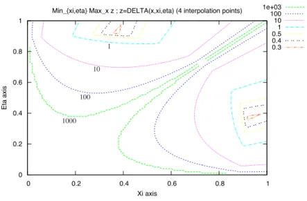
For n= 3, the four interpolation points form a symmetrical set {±&, ±*}. Hence the optimization is made over two parameters& and*. Thus, the function
Min_{xi,eta} Max_x z ; z=DELTA(x,xi,eta) (4 interpolation points) 1e+03 100 10 1 0.5 0.4 0.3 0 0.2 0.4 0.6 0.8 1 Xi axis 0 0.2 0.4 0.6 0.8 1 Et a a xi s 1000 100 10 1
Fig. 1 Contour plot of function z(& , *) of (59) for n + 1 = 4: the plot is symmetrical w.r.t. the
bisecting line* = & , and one location of the minimum is & = 0.351, * = 0.926
z(*,*) = max
x∈[0,1],(x) (59)
is defined discretely. The iso-value contours of this function are indicated in Fig. 1, which permits after refinement to identify the optimum& ≈ 0.351 and*≈ 0.926.
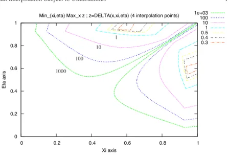
For n= 4, the five interpolation points form a symmetrical set 0, {±&, ±*}. Hence the optimization is again made over two parameters& and*. Thus, the func-tion z(*,*) is again defined by (59) and evaluated discretely. The iso-value contours of this function are indicated in Fig. 2, which permits after refinement to identify the optimum&≈ 0.571 and*≈ 0.948.
4.4 General Results (n
> 4)
The min-max-, problem has been solved by either analytical or numerical means for values of n in the range from 0 to 40. The results are collected in Table 1 in which the first column indicates the number of interpolation points n+ 1, the second gives the definition of the Chebyshev points&⋆(n≤ 4), the third provides the definition of the optimal distribution &, and the fourth a comparison of performance by giving, when available, the values of
1. ,= maxx,(x, &), the upper bound on,(x) corresponding to the optimal
Min_{xi,eta} Max_x z ; z=DELTA(x,xi,eta) (4 interpolation points) 1e+03 100 10 1 0.5 0.4 0.3 0 0.2 0.4 0.6 0.8 1 Xi axis 0 0.2 0.4 0.6 0.8 1 Et a a xi s 1000 100 10 1
Fig. 2 Contour plot of function z(& , *) of (59) for n + 1 = 5: the plot is symmetrical w.r.t. the
bisecting line* = & , and one location of the minimum is & = 0.571, * = 0.948
2. ,⋆= max
x,(x,&⋆), the upper bound on ,(x) corresponding to the
approxi-mately optimal distribution&=&⋆of interpolation points (the Chebyshev dis-tribution);
3. ,u= max
x,(x,&u), the upper bound on ,(x) corresponding to the uniform
distribution&=&uof interpolation points.
The analytical results are related to the cases for which n≤ 4, and have been outlined in a previous subsection.
For n+ 1 ≥ 10, the distribution &(not given here) has been identified by a numer-ical minimization realized by a particle-swarm (PSO) algorithm. The table indicates the corresponding values of ,.
From these results, one observes that the upper bound , achieved when the dis-tribution of interpolation points is optimized, is not only bounded, but it even di-minishes with increasing n. The Chebyshev distribution has an almost equivalent performance. Inversely, the uniform distribution yields a value of the upper bound
,uthat is unbounded with n. In conclusion, using the Chebyshev distribution, which
is known explicitly, is highly recommended in practice.
5 Generalized Hermitian Interpolation
In this section, we generalize the notions introduced in the first three to the situation where one wishes to construct a(the) low(est)-degree polynomial interpolant of the values, as well as the derivatives up to order, say p (p∈ N), of a given smooth
Table 1 Variation of the criterion maxx, (x, & ), related to Hermitian interpolation with uncertain derivatives, for different choices of the set& = {&i}, i = 1, ..., n, of interpolation points in [−1,1], and different degrees, 2n+ 1; , = maxx, (x, & ), ,⋆= maxx, (x, &⋆) and ,u= maxx, (x, &u), where&u i = −1 +n−12 (i − 1), i = 1,...,n. Number interpol. pts.: n+ 1 Degree of interpolant: 2n+ 1 Chebyshev points:&⋆ & = arg min&maxx,
Performance: , ,⋆ ,u 1 1 0 0 1 1 1 2 3 ± 1 √ 2 . = ±0.7071 ±0.7549 0.37740.5 0.5 3 5 0 ±√3 2 . = ±0.8660 0 ±0.8677 0.3258 0.3333 0.3755 4 7 ±41 2−√18 . = ±0.3827 ±41 2+√18 . = ±0.9239 ±0.351 ±0.926 0.282 0.299 0.439 5 9 0 ± 4 5−√5 8 . = ±0.5878 ± 4 5+√5 8 . = ±0.9511 0 ±0.571 ±0.948 0.249 0.262 0.652 10 19 0.164 0.179 39. 11 21 0.154 0.167 111. 20 39 0.103 0.112 3.9 × 10⁶ 21 41 0.100 0.108 1.3 × 10⁷
function f(x) over [−1,1]. The interpolation points are again denoted {xi}i=0,1,...,n, and we use the notation
y(k)i = f(k)(xi), k= 0, 1, ..., p; i = 0, 1, ..., n. (60)
The interpolation polynomial is denoted Hn,p(x) and it is now constrained to the following(p + 1)(n + 1) interpolation conditions:
∀k ∈ {0,1,..., p}, ∀i ∈ {0,1,...,n} : H(k)n,p(xi) = y(k)i . (61)
We associate such kind of interpolation with the expression “generalized Hermitian interpolation”.
5.1 Existence and Uniqueness
We first establish existence and uniqueness by the following:
Theorem 1. There exists a unique polynomial Hn,p(x) of degree at most equal to (p + 1)(n + 1) − 1 satisfying the generalized interpolation conditions (61).
Proof. By recurrence on p. For p= 0, the generalized Hermitian interpolation reduces to the classical Lagrange interpolation, whose solution is indeed unique among polynomials of degree at most equal to(p + 1)(n + 1) − 1 = n:
Hn,0(x) = Pn(x). (62)
For p≥ 1, assume Hn,p−1(x) exists and is unique among polynomials of degree at most equal to p(n + 1) − 1. This polynomial, by assumption, satisfies the following interpolation conditions:
∀k ∈ {0,1,..., p − 1}, ∀i ∈ {0,1,...,n} : H(k)n,p−1(xi) = y(k)i . (63)
Hence, by seeking Hn,p(x) in the form
Hn,p(x) = Hn,p−1(x) + R(x), (64)
one finds that R(x) should be of degree at most equal to (p + 1)(n + 1) − 1 and satisfy
∀k ∈ {0,1,..., p − 1}, ∀i ∈ {0,1,...,n} : R(k)(xi) = 0 (65)
and
∀i ∈ {0,1,...,n} : R(p)(xi) = y(p)i − H(p)n,p−1(xi). (66)
Now, (65) is equivalent to saying that R(x) is of the form
R(x) =
n
#
i=0
(x − xi)p· Q(x) ="(x)pQ(x) (67)
for some quotient Q(x). Then, the derivative of order p of R(x) at x = xiis calculated
by the Leibniz formula applied to the product u(x)v(x) where
u(x) = (x − xi)p, v(x) = n
#
j=0 j#=i (x − xj)p· Q(x). (68) This gives R(p)(xi) = p%
k=0 . p k / u(k)(xi) v(p−k)(xi). (69)R(p)(xi) = p! v(xi) = p! n
#
j=0 j#=i (xi− xj)pQ(xi) = p!"′(xi)pQ(xi) . (70)Thus, all the interpolation conditions are satisfied iff the polynomial Q(x) fits the following interpolation conditions:
∀i ∈ {0,1,...,n} : Q(xi) = Qi=
R(p)(xi)
p!"′(xi)p=
y(p)i − H(p)n,p−1(xi)
p!"′(xi)p . (71)
Therefore, solutions exist, and the lowest-degree solution is uniquely obtained when
Q(x) is the Lagrange interpolation polynomial associated with the above function values. This polynomial is of degree at most equal to n. Hence, R(x) and Hn,p(x) are of degree at most equal to p(n + 1) + n = (p + 1)(n + 1) − 1. !
5.2 Interpolation Error and Best Approximation
We have the following:
Theorem 2 (Interpolation error associated with the generalized Hermitian inter-polant). Assuming that f∈ C(p+1)(n+1)([−1,1]), we have
∀x ∈ [−1,1], ∃& ∈ [−1,1] : f (x) = Hn,p(x) +"(x)p+1
f([(p+1)(n+1)])(&) [(p + 1)(n + 1)]!. (72)
Proof. Let x∈ [−1,1] be fixed. If x = xifor some i∈ {0,1,...,n}, f (x) = Hn,p(x) and"(x) = 0, and the statement is trivial. Hence, assume now otherwise that x #= xi
for any i∈ {0,1,...,n}. Then, define the constant
.= f(x) − Hn,p(x)
"(x)p+1 (73)
so that
f(x) = Hn,p(x) +."(x)p+1. (74)
Now using the symbol t for the independent variable, one considers the function
)(t) = f (t) − Hn,p(t) −."(t)p+1. (75) By virtue of the interpolation conditions satisfied by the polynomial Hn,p(t),
∀k ∈ {0,1,..., p}, ∀i ∈ {0,1,...,n} : )(k)(xi) = 0 (76)
but, additionally, by the choice of the constant., we also have
This makes n+ 2 distinct zeroes for)(x) : x0, x1, ..., xnand x. Thus, by application
of Rolle’s theorem in each of the n+ 1 consecutive intervals that these n + 2 points once arranged in an increasing order define, a zero of)′(t) exists, yielding n + 1 distinct zeroes for)′(t), to which (76) adds n + 1 distinct and different ones, for a total of 2(n + 1) = 2n + 2 zeroes. Strictly between these, one finds 2(n + 1) − 1 zeroes of)′′(t) to which (76) adds n + 1 distinct and different ones, for a total of 3(n + 1) − 1 = 3n + 2 zeroes. Thus, for every new derivative, we find one less zero in every subinterval, but n+ 1 more by virtue of (76), for a total of n more, and this as long as (76) applies. Hence we get that)(p)(t) admits at least (p + 1)n + 2 distinct zeroes. For derivatives of higher order, the number of zeroes is one less for every new one; hence,(p + 1)n + 1 for )(p+1)(t), and so on. We finally get that )([p+(p+1)n+1])(t) =)([(p+1)(n+1)])(t) admits at least one zero&, that is
0= f([(p+1)(n+1)])(&) −.[(p + 1)(n + 1)]! (78) because H([(p+1)(n+1)])(&) = 0 since the degree of Hn,p(t) is at most equal to (p + 1)(n + 1) − 1, and the conclusion follows. !
As a consequence of this result, it is clear that the best generalized Hermitian ap-proximation is achieved by the Chebyshev distribution of interpolation points again.
5.3 Best Inexact Generalized Hermitian Interpolation
Now suppose that all the data on f and its successive derivatives are exact, ex-cept for the derivatives of the highest order,{y(p)i } that are subject to uncertainties {!i}i=0,1,...,n. Then, the uncertainties on the values{Qi}i=0,1,...,nof the quotient Q(x) are the following:
$Qi=
!i
p!"′(xi)p; (79)
on the quotient itself the following:
$Q(x) = n
%
i=0 !i p!"′(xi)pLi(x) ="(x) n%
i=0 !i p!"′(xi)p+1(x − x i) ; (80)and, finally, the uncertainty on the generalized Hermitian interpolant Hn,p(x) the following: $Hn,p(x) ="(x)p+1 n
%
i=0 !i p!"′(xi)p+1(x − x i) . (81)In conclusion, for situations in which the uncertainties{!i}i=0,1,...,nare bounded by the same number!, the criterion that one should consider to conduct the min-max optimization of the interpolation points{xi}i=0,1,...,nis now the following one to replace the former,(x):
,(p)(x) = |"(x)|p+1 n
%
i=0 1 p!|"′(xi)|p+1 |x − xi| (82) or, equivalently, p+14 ,(p)(x) = |"(x)| p+1 5 n%
i=0 1 p!|"′(xi)|p+1 |x − xi| . (83)We note that this expression is a homogeneous function of"(x) of degree 0. We conjecture that the variations of the above criterion, as p→ /, are domi-nated by those of the factor|"(x)|. Hence, in this limit, the optimal distribution of interpolation points should approach the Chebyshev distribution.
5.4 Overall Bound on the Approximation Error
The quantity !,(p)(x) is an absolute bound on the error committed in the com-putation of the generalized Hermitian interpolant based on function and derivative values in presence of uncertainties on the derivatives of the highest order, p, only, when these are uniformly bounded by!:
∀x ∈ [−1,1] : !!$Hn,p(x) ! != ! ! Hn,p(x) − Hn,p(x) ! !≤!,(p)(x), (84)
where Hn,p(x) represents the actually computed approximation.
On the other hand, the interpolation error is the difference between the actual function value, f(x), and the “true” interpolant, Hn,p(x), that could be computed if all function and derivative information was known. The interpolation error satisfies
∀x ∈ [−1,1] : ! !f(x) − Hn,p(x)!!= ! ! ! ! ! "(x)p+1f ([(p+1)(n+1)])(&) [(p + 1)(n + 1)]! ! ! ! ! ! ≤µn,p|"(x)|p+1, (85) where one has let
µn,p= max x∈[−1,1] ! ! ! ! ! f([(p+1)(n+1)])(x) [(p + 1)(n + 1)]! ! ! ! ! ! . (86) Consequently, we have ∀x ∈ [−1,1] : ! !f(x) − Hn,p(x) ! !≤µn,p|"(x)|p+1+!,(p)(x). (87) Now, examining the precise expression for,(p)(x), that is (82), we see that the ratio of the second term to the first on the right of the above inequality is equal to
! µn,p n
%
i=0 1 p!|"′(xi)|p+1 |x − xi| . (88)For given n and p, this expression is unbounded in x. Thus, (the bound on) the error is inevitably degraded in the order of magnitude due to presence of uncertainties.
However, the actual dilemma of interest is somewhat different. It is the following: given the values{yi, y′i, ..., y(p−1)i }, 0 ≤ i ≤ n, and correspondingly, approximations
of the higher derivative{y(p)i }, which of the following two interpolants is (guaran-teed to be) more accurate:
1. the Hermitian interpolant of the sole exact values:{yi, y′i, ..., y(p−1)i }, 0 ≤ i ≤ n,
or
2. the Hermitian interpolant of the entire data set?
The first interpolant differs from f(x) by the sole interpolation error,µn,p−1|"(x)|p. The second interpolant is associated with the higher-order interpolation error,
µn,p|"(x)|p+1, but is subject to the uncertainty term!,(p)(x), which is dominant, as we have just seen. Thus, the decision of whether to include derivatives or not should be guided by the ratio of the uncertainty term,!,(p)(x), to the lower interpolation error,µn,p−1|"(x)|p. This ratio is equal to
! µn,p−1|"(x)| n
%
i=0 1 p!|"′(xi)|p+1 |x − xi| (89) and it admits the bound!Bn,p
µn,p−1, (90)
where the bound
Bn,p= max x∈[−1,1]|"(x)| n
%
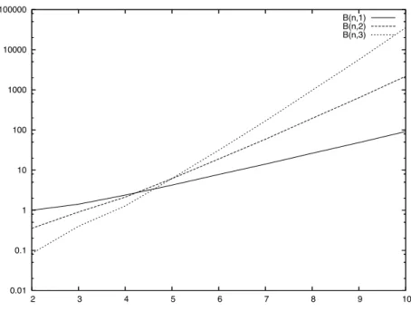
i=0 1 p!|"′(xi)|p+1 |x − xi| (91) exists since, in the above, the function over which the max applies is piecewise polynomial for fixed n and p.Hermitian interpolation is definitely preferable whenever the expression in (90) is less than 1. This criterion permits us to identify trends as!, n and p vary, but is not very practical in general since the factors! andµn,p−1are problem-dependent and out of control. The variation with n of the bound Bn,phas been plotted in Fig. 3 for p= 1, 2 and 3. Visibly, the bound Bn,p can be large unless p and n are small. Therefore, unsurprisingly, unless n and p, as well as the uncertainty level !, are small enough, the criterion in (90) is larger than 1, and the interpolant of the sole exactly known values is likely to be the more accurate one.
To appreciate this in a practical case, we have considered the case of the interpo-lation of the function
f(x) = f'(x) = 1
1+'x2 (92)
over the interval[−1,1] for p = 0 (Lagrange interpolation) and p = 1 (Hermitian interpolation). This smooth function is bounded by 1, and its maximum derivative
0.01 0.1 1 10 100 1000 10000 100000 2 3 4 5 6 7 8 9 10 B(n,1) B(n,2) B(n,3)
Fig. 3 Coefficient Bn,pas a function of n for p= 1, 2 and 3
increases with'. For'= 64/27, this maximum is equal to 1. For'= 256/27, this maximum is equal to 2.
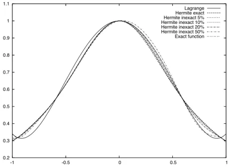
In the first experiment (Figs. 4 and 5), ' = 64/27 and n = 5. The Lagrange interpolant is fairly inaccurate, mostly near the endpoints. Thus the error distribution indicates that the approximate Hermitian interpolant is preferable even for a fairly high level of uncertainty on the derivatives (20 % is acceptable).
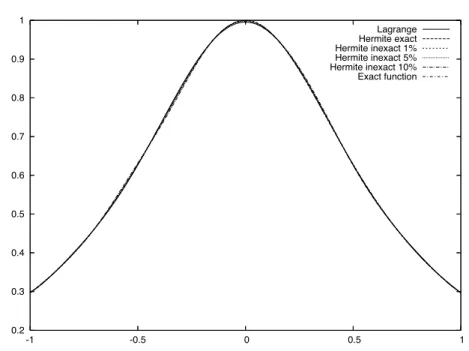
In the second experiment (Figs. 6 and 7), the interpolated function is the same, but the number n is doubled (n= 10). Consequently, the Lagrange interpolant of the sole exact function values is very accurate. The approximate Hermitian interpolant can only surpass it if the level of uncertainty on the derivatives is small (less than 5 %).
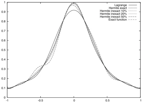
Lastly, with the same number of interpolation points (n= 10), we have consid-ered the case of a function with larger derivatives (' = 256/27). As a result (see Figs. 8 and 9), the accuracy of the Lagrange interpolation has been severely de-graded. Then again, the approximate Hermitian interpolation is found superior for higher levels of uncertainty in the derivatives (the switch is between 20 and 50 %).
0.2 0.3 0.4 0.5 0.6 0.7 0.8 0.9 1 1.1 -1 -0.5 0 0.5 1 Lagrange Hermite exact Hermite inexact 5% Hermite inexact 10% Hermite inexact 20% Hermite inexact 50% Exact function
Fig. 4 Case' = 64/27 (maxx| f'(x)| = maxx
! !f'′(x)
!
!= 1); function f'(x) and various interpola-tion polynomials (n= 5) -0.06 -0.04 -0.02 0 0.02 0.04 0.06 0.08 -1 -0.5 0 0.5 1 Error Lagrange Error Hermite exact Error Hermite inexact 50% Error Hermite inexact 20% Error Hermite inexact 10% Error Hermite inexact 5%
Fig. 5 Case' = 64/27 (maxx| f'(x)| = maxx
! !f'′(x)
!
!= 1); error distribution associated with the various interpolation polynomials (n= 5)
0.2 0.3 0.4 0.5 0.6 0.7 0.8 0.9 1 -1 -0.5 0 0.5 1 Lagrange Hermite exact Hermite inexact 1% Hermite inexact 5% Hermite inexact 10% Exact function
Fig. 6 Case' = 64/27 (maxx| f'(x)| = maxx
! !f'′(x)
!
!= 1); function f'(x) and various interpola-tion polynomials (n= 10) -0.008 -0.006 -0.004 -0.002 0 0.002 0.004 0.006 0.008 -1 -0.5 0 0.5 1 Error Lagrange Error Hermite exact Error Hermite inexact 10% Error Hermite inexact 5% Error Hermite inexact 1%
Fig. 7 Case' = 64/27 (maxx| f'(x)| = maxx
! !f'′(x)
!
!= 1); error distribution associated with the various interpolation polynomials (n= 10)
0 0.1 0.2 0.3 0.4 0.5 0.6 0.7 0.8 0.9 1 -1 -0.5 0 0.5 1 Lagrange Hermite exact Hermite inexact 10% Hermite inexact 20% Hermite inexact 50% Exact function
Fig. 8 Case' = 256/27 (maxx| f'(x)| = 1; maxx
! !f'′(x)
!
!= 2); function f'(x) and various inter-polation polynomials (n= 10) -0.1 -0.08 -0.06 -0.04 -0.02 0 0.02 0.04 0.06 0.08 -1 -0.5 0 0.5 1 Error Lagrange Error Hermite exact Error Hermite inexact 10% Error Hermite inexact 20% Error Hermite inexact 50%
Fig. 9 Case' = 256/27 (maxx| f'(x)| = 1; maxx
! !f'′(x)
!
!= 2); error distribution associated with the various interpolation polynomials (n= 10)
6 Conclusions
Recalling that the Chebyshev distribution of interpolation points is optimal w.r.t. the minimization of the (known bound on the) interpolation error, we have proposed an alternate criterion to be subject to the min-max optimization. The new criterion to be minimized aims at reducing the sensitivity of the Hermitian interpolant of func-tion values and derivatives, to uncertainties assumed to be present in the derivatives only. We have found by analytical developments and numerical experiments that the Chebyshev distribution is close to be optimum w.r.t. this new criterion also, thus giving the stability of the corresponding approximation a somewhat larger sense.
We have also considered the generalized Hermitian interpolation problem in which the derivatives up to some order p (p> 1) are fitted. For this problem we have derived the existence and uniqueness result, as well as the expression of the interpolation error, and also the definition that one could use for the criterion to be subject to the min-max optimization to reduce the sensitivity of the interpolant to uncertainties in the derivatives of the highest order. We conjectured from the de-rived expression that the corresponding optimal distribution of interpolation points converges to the Chebyshev distribution as p→ /.
Lastly, we have made actual interpolation experiments in cases of a function bounded by 1, whose derivative is either bounded by 1 or 2. These experiments have confirmed that the approximate Hermitian interpolant was superior to the Lagrange interpolant of the sole exact function values, when the uncertainty on the derivatives is below a certain critical value which decreases when n is increased.
In perspective, we intend to examine a much more complicated case in which the meta-model depends nonlinearly on the adjustable parameters, by means of semi-formal or numerical analysis tools.
References
1. M. Bompard, J.-A. D´esid´eri, and J. Peter. Best Hermitian interpolation in presence of uncer-tainties. INRIA Research Report 7422, Oct. 2010. (http://hal.inria.fr/inria-00526558/en/). 2. S. D. Conte and C. de Boor. Elementary numerical analysis: An algorithmic approach.
McGraw-Hill, New York, second edition, 1972.
3. D. Jones. A taxonomy of global optimization methods based on response surfaces. Journal of
Global Optimization, 21(4):345–383, 2001.
4. C. E. Pearson, editor. Handbook of applied mathematics: Selected results and methods. Van Nostrand Reinhold, New York, second edition, 1990.
5. A. Quarteroni, R. Sacco, and F. Saleri. Numerical mathematics. Number 37 in Texts in Applied Mathematics. Springer, Berlin, second edition, 2007.
6. J. Sacks, W. Welch, T. Mitchell, and H. Wynn. Design and analysis of computer experiments.
![Table 1 Variation of the criterion max x ,(x,& ), related to Hermitian interpolation with uncertain derivatives, for different choices of the set & = {& i }, i = 1, ..., n, of interpolation points in [ − 1,1], and different degrees, 2n + 1; ,](https://thumb-eu.123doks.com/thumbv2/123doknet/13367954.403645/15.892.197.706.218.680/variation-criterion-hermitian-interpolation-uncertain-derivatives-different-interpolation.webp)