HAL Id: halshs-02354576
https://halshs.archives-ouvertes.fr/halshs-02354576
Submitted on 7 Nov 2019
HAL is a multi-disciplinary open access
archive for the deposit and dissemination of sci-entific research documents, whether they are pub-lished or not. The documents may come from teaching and research institutions in France or abroad, or from public or private research centers.
L’archive ouverte pluridisciplinaire HAL, est destinée au dépôt et à la diffusion de documents scientifiques de niveau recherche, publiés ou non, émanant des établissements d’enseignement et de recherche français ou étrangers, des laboratoires publics ou privés.
Monetary Dynamics in a Network Economy
Antoine Mandel, Vipin Veetil
To cite this version:
Documents de Travail du
Centre d’Economie de la Sorbonne
Monetary Dynamics in a Network Economy Antoine MANDEL, Vipin P. VEETIL
Monetary Dynamics in a Network Economy
Antoine Mandel
úVipin P. Veetil
†October 4, 2019
Abstract
We develop a tractable model of out-of-equilibrium dynamics in a general equilibrium economy with cash-in-advance constraints. The dynamics emerge from local interactions between firms governed by the production network underlying the economy. We analytically characterise the influence of network structure on the propagation of monetary shocks. In the long run, the model converges to general equilibrium and the quantity theory of money holds. In the short run, monetary shocks propagate upstream via nominal demand changes and downstream via real supply changes. Lags in the evolution of supply and demand at the micro level can give rise to arbitrary dynamics of the distribution of prices. Our model explains the long standing Price Puzzle: a temporary rise in the price level in response to monetary contractions. The Price Puzzle emerges under two assumptions about downstream firms: they are disproportionally affected by monetary contractions and they account for a sufficiently small share of the wage bill. Empirical evidence supports the two assumptions for the US economy. Our model calibrated to the US economy using a data set of more than fifty thousand firms generates the empirically observed magnitude of the price level rise after monetary contractions.
JEL Codes C63, C67, D80, E31, E52
Key Words Price Puzzle, Production Network, Money, Monetary Non-Neutrality,
Out-of-Equilibrium Dynamics.
úParis School of Economics, Universit´e Paris 1 Panth´eon-Sorbonne. Maison des Sciences ´Economiques, 106-112 Boulevard de l’hˆopital 75647 Paris Cedex 13, France.
†Department of Humanities and Social Sciences, Indian Institute of Technology Madras, Chennai, India 600036.
1 Introduction
A basic implication of the quantitative theory of money is that monetary contractions induce a decrease in the price level. However, numerous empirical studies report monetary contractions generate a temporary increase in the price-level. This “price puzzle” is sizeable: a monetary contraction that generates a 0.1% decrease in the price-level in three years is capable of generating a 0.1% increase in three months (Rusnak et al., 2013, Table 4). The sizeable wrong directional movement in the price-level is significant because the price-level mediates the relation between money and output in theoretical models of monetary neutrality (Lucas, 1972; Ball and Mankiw, 1994). Within sticky-price and sticky-information models of monetary neutrality, a wrong directional change in the price-level implies a counterfactual relation between money and output (Mankiw and Reis, 2002). The Price Puzzle is therefore empirically sizeable and theoretically significant.
This paper argues that the price puzzle emerges from the out-of-equilibrium propagation of monetary shocks through the production network of the economy. The propagation of monetary shocks generate differential and time-varying responses in the supply and demand for consumer goods. The price puzzle emerges if monetary shocks have a strong short-term impact on the supply and a weak short-short-term impact on the demand of consumption goods. Two conditions prove sufficient to induce these dynamics: downstream firms must be disproportionally affected by monetary contractions and they must account for a sufficiently small share of the wage bill. Both conditions find empirical support. Also, our model calibrated to the US economy generates the empirically observed magnitude of the wrong directional movement in the price-level following a moonetary contraction.
Our approach builds on Acemoglu et al.’s (2012) model of the network origins of aggregate fluctuations. We consider an economy with a representative consumer and a finite number of firms with Cobb-Douglas production functions. The production network of the economy is identified with the weights of these Cobb-Douglas functions. We introduce two novel elements in this framework. First, we study out-of-equilibrium dynamics in which prices are set locally by firms. Second, motivated by the empirical observation that firms’ liquidity can be binding and theoretical insights on the macro-economic implications of these constraints (Grossman and Weiss, 1982; Stiglitz, 1988; Aghion et al., 2012), we study firms with cash-in-advance constraints as in Lucas and Stokey (1985). These assumptions together make the out-of-equilibrium dynamics tractable by generating linear dynamics in money balances. In the long run, the quantity theory of money holds as the model converges to the general equilibrium pertaining to the underlying primitives. In the short run, monetary disequilibrium propagates upstream via nominal demand changes and downstream via real supply changes.
Monetary shocks take the form of heterogeneous lump-sum transfers of money (Levine, 1991; Molico, 2006; Anthonisen, 2013). We investigate the impact of monetary shocks on the demand and supply for consumer goods in the course of out-of-equilibrium dynamics generated by the shocks. The demand for consumer goods comes from a representative household. The supply for consumer goods comes from a subset of firms. We define the price level as a weighted mean of the price of consumer goods. A monetary contraction affects both the demand and the supply of consumer goods but through different mechanisms and with different time lags. On the demand side, firms hurt by the initial impact and subsequent propagation of a monetary contraction decrease wages. The decrease in wages decreases the
household’s income and therefore the demand for consumer goods. The time necessary for a monetary contraction to generate the long run decrease in nominal demand for consumer goods depends on the topology of the production network and the distribution of labor among firms. On the supply side, firms hurt by a monetary contraction and its propagation temporarily decrease their output as their inputs are bid away by competing users. This decrease in output propagates downstream through the production network1.
In the long run, monetary contractions have no effect on the real demand and supply of consumer goods as the economy reaches a new equilibrium with a lower price level. Our model generates long run neutrality of money with respect to all real variables. But it generates short run non-neutrality as the propagation of monetary contractions generates a temporary increase in the price level. We analytically characterise two conditions under which the model generates a wrong directional change in the price level. The first condition is firms hurt by monetary contractions are sufficiently downstream. This condition guarantees that monetary contractions generate a decrease in the supply of consumer goods. The second condition is firms hurt by monetary contractions bear a sufficiently small share of the economy’s wage bill. This condition guarantees that monetary contractions take sufficient time to generate the long run decrease in the nominal demand for consumer goods.
Theory and data support the two aforementioned conditions. The first condition follows from the joint observation that downstream firms are disproportionately small and small firms are disproportionately hurt by monetary contractions. The share of small firms in basket of consumer goods is more than twice their share in the economy. Small firms not only have a disproportionately high role in the production of consumer goods, they are also more hurt by monetary contractions (Gertler and Gilchrist, 1994; Gaiotti and Generale, 2002; Iyer et al., 2013; Carb´o-Valverde et al., 2016). One reason small firms are more hurt by monetary contractions is their inability to substitute external finance with internal funds (Greenwald and Stiglitz, 1993; Holmstrom and Tirole, 1997; Clementi and Hopenhayn, 2006).
Overall, there exist empirical and theoretical reasons which explain the temporary decrease in the supply of consumer goods in response to monetary contractions. Our second condition emphasizes that nominal demand decreases slowly because small firms which bear the brunt of the initial impact of monetary contractions account for a limited portion of the economy’s wage bill. Firms with annual receipts of less than one million account for less than 8% of the wage bill in the US economy. Therefore the initial impact of a monetary contraction generates a limited decrease in wages. Studies on household behavior also suggest that in the short run demand for consumption goods decreases less than proportionally to changes in income (Hall, 1978; Altonji and Siow, 1987; Jappelli and Pistaferri, 2010). Though our model does not incorporate consumption smoothening, it is an additional reason why the decrease in final demand is slow in the short run.
We investigate the empirical validity of the model by calibrating it on the US production network using a novel data set with more than 100,000 buyer-seller relations between more than 50,000 US firms including all major publicly listed firms. We use Monte Carlo methods to study the dynamics of the calibrated synthetic economy with computational experiments.
1A collorollary of the argument is that a monetary contraction can increase the supply of consumer goods if firms most hurt by the shock are sufficiently upstream. When firms far upstream are hurt by a monetary contraction, downstream firms purchase more of the inputs used by both sets of firms by outbidding upstream firms. This allows downstream firms to expand the output of consumer goods.
In the experiments, the initial impact of monetary shock scales sublinearly with firm size: small firms are disproportionately hurt by contractions. The model calibrated to the US production network robustly reproduces the empirically observed magnitude of the increase in price level after monetary contractions.
1.1 Related literature
While the phrase “Price Puzzle” was coined by Eichenbaum’s (1992), the empirical phenomena marked by the phrase was first noted by Thomas Tooke more than a century and a half ago. The wrong directional movement in the price level which Eichenbaum called the Price Puzzle has been found in a number of economies including Australia, France, Germany, India, Italy, Japan, United Kingdom, and the United States (Sims, 1992; Gaiotti and Secchi, 2006; Mishra and Mishra, 2012; Bishop and Tulip, 2017). Sims and Eichenbaum’s statement of the problem generated a flurry of empirical work that attempted to identify variables whose inclusion in VAR models would eliminate the price puzzle. Some suggested variables pertaining to commodity prices and the private information with central banks may help resolve the Puzzle. These variables have had limited success. More specifically, the methods which dampen or eliminate the Price Puzzle in some periods, do not do so for others (Demiralp et al., 2014). For instance, Barakchian and Crowe (2013) find the methods which generate right directional price level changes through the mid-1990s, generate wrong directional price level changes when estimated over later samples (particularly in the first year after monetary shocks). The problem is so pervasive that some economists have had to allow control variables in VAR models to take different coefficients for different subsample periods (Jorda and Taylor, Forthcoming). Rusnak et al. (2013) present a meta analysis of the empirical literature on the subject. They find that about 50% of modern studies find a temporary rise in the price level following a monetary contraction after controlling for a variety of variables. Similarly, Ramey (2016, p. 36) finds most models of monetary policy shocks “are plagued by the Price Puzzle
to greater or lesser degree” (see Table 3.1 in her paper).
As Sims (1992, p. 975) noted long ago, the tendency of a monetary contraction to predict high inflation is hard “to reconcile with effective monetary policy”. Numerous economists therefore attempted to develop theoretical explanations of the Price Puzzle. Most expla-nations fall within one of three groups: “common factors hypothesis”, “reverse causation hypothesis”, and the “cost channel hypothesis”. The common factors hypothesis states price level increase and monetary contraction are driven by common factors (Brown and Santoni, 1987). The common factors are typically estimated using econometric techniques with little theoretical motivation (Bernanke et al., 2005). The empirical performance of the common factors hypothesis is mixed. In a meta analysis of empirical studies on the Price Puzzle, Rusnak et al. (2013) find that eight of eleven estimates using factor augmented VAR exhibit the Price Puzzle.
The reverse causation hypothesis states present monetary contraction is caused by future increase in the price level (Brissimis and Magginas, 2006; Barakchian and Crowe, 2013; Cloyne and H¨urtgen, 2016). More specifically, present monetary contraction is a consequence of a policy decision based on an expectation of a future increase in the price level. Thapar (2008) however finds the Price Puzzle to be present even after conditioning for the information
set of central banks. And Hanson (2004) finds no correlation between a variable’s ability to forecast inflation and its ability to resolve the Price Puzzle. Ramey (2016) re-estimates several models to control for all information available to the Federal Reserve. Her estimates show that the wrong directional movement in the price level does not dampen due to the expansion of the information set, in fact it increases the price puzzle. The reverse causation hypothesis therefore finds limited empirical support.
The cost channel explanation of the Price Puzzle was first proposed by Thomas Tooke. He argued that an increase in the interest rate increases the cost of production and therefore the price level. Barth III and Ramey (2001) present a model of the cost channel explanation. One of the problems with the cost channel explanation is that it involves an inadmissible use of ceteris paribus conditions. An exogenous increase in the cost of one factor of production will necessarily decrease expenditures on other factors of production, thereby generating a decrease in some prices: this follows from the equation of exchange (Laidler, 1991). Prima facia there is little reason to believe the prices which increase through the cost-channel are disproportionately represented in the Consumer Price Index and Personal Consumption Expenditure Index. This is why Wicksell (1935, p. 182-184) thought “Tooke’s thesis is certainly wrong”. Our explanation of the Price Puzzle refines the cost channel mechanism so as to resolve Wicksell’s criticism. Our theory is consistent with Wicksell’s (1958) assertion that rise in prices of some goods will be compensated for by the fall in prices of other goods in so far as neither the quantity nor the velocity of money change. Furthermore, since a negative monetary shocks entails a decrease in the quantity of money, the rise in prices of some goods must be more than compensated for by the fall in prices of other goods. Our theory presents an explanation for why those goods whose prices rise happen to be disproportionately represented in basket of consumer goods.
In resolving the Price Puzzle, we show price dynamics are intimately related to the size distribution of firms within the production network. Our emphasis on firm size distribu-tion echoes Gabaix’s (2011) claim that the granular structure of an economy plays a role in generating macroeconomic phenomena. In essence we formalise a novel mechanism for generating monetary non-neutrality: the percolation of monetary shocks through the produc-tion network. Our paper is therefore thematically akin to recent work on ‘micro to macro via production networks’ (Carvalho and Tahbaz-Salehi, 2018). Over the years economists developed numerous monetary transmission mechanisms2. Few however made the production
network the focal point of analysis, with the notable exception of Cantillon (1755), Mises (1953), and Friedman (1961). Among contemporary contributions, Nakamura and Steinsson (2010) and Paston et al. (2018) show intermediate inputs amplify the impact of monetary shocks. Anthonisen (2010) formalises monetary dynamics on production networks using an overlapping generations model. And Mandel et al. (2019) study price dynamics on production networks using an agent-based computational model. Ozdagli and Weber (2017) present the only notable empirical measure of the role of production network in transmitting monetary 2Monetary transmission mechanisms include money illusion (Shafir and Tversky, 1997; Fehr and Tyran, 2001), the presence of a small number of price-wage setters (Soskice and Iversen, 2000), asyncrhonized price setting (Caplin and Spulber, 1987), slow dissemination of information about the state of the economy (Lucas, 1972; Mankiw and Reis, 2002), the institutional structure of the banking system (Saving, 1973), transactions costs (Rotemberg, 1984), incomplete asset markets (Gottardi, 1994), inflexible labor contracts (Cooper, 1988), and differences in beliefs about the price level (King, 1982; Chwe, 1999).
shocks. They attribute 50-85% of the real effect of monetary shocks to propagation through the production network. Preliminary empirical evidence therefore suggests the production network is a significant transmission mechanism.
One of the principle contributions of this paper is that we analytically characterize the out-of-equilibrium dynamics which emerge from asymmetric initial impact of monetary shocks. In this sense our work combines recent work on networks with older work on non-Walrasian monetary economics (Lucas and Woodford, 1993; Eden, 1993). Numerous economists before us have developed models in which non-neutralities emerge from asymmetric injections (Scheinkman and Weiss, 1986; Fuerst, 1992; Christiano and Eichenbaum, 1995; Alvarez et al.,
2002; Williamson, 2008). Most models of asymmetric injections however assume agents rebalance their money holdings by accessing Walrasian markets (Berentsen et al., 2005). Within our model agents readjust their money balances using decentralised out-of-equilibrium trades. The number of trades necessary for all agents to readjust their real money balances is an endogenous variable which depends on the second Eigenvalue of the production network. In other words, the time it takes for the economy to reach a new equilibrium after a monetary shock depends on the second of eigenvalue the production network.
The rest of the article is organized as follows. Section 2 presents the model. Section 3 analytically characterizes the propagation of monetary shocks in the model and states sufficient conditions for the price level to increase after a monetary contraction. Section 4 presents the results of simulations performed with the model calibrated to granular data on more than 100,000 buyer-seller relations between more than 50,000 US firms. Section 5 concludes the paper. Proofs are in the Appendix.
2 Model
2.1 The general equilibrium framework
We consider a general equilibrium economy as in Acemoglu et al. (2012) with a finite number of firms and a representative household. The firms and the differentiated goods they produce are indexed by M = {1,··· ,n}. The household has index 0 and N = {0,··· ,n} denotes the set of agents. The representative household inelastically supplies ⁄0 units of labor and has a
Cobb-Douglas utility function of the form:
u(x1,··· ,xn) :=
Ÿ
jœM
xaij,0 (1)
where for all j œ M, aj,0 œ R+ is the share of good j in the household’s consumption
expenditures, thus qjœMaj,0= 1.
Each firm i œ M has a Cobb-Douglas production function of the form
fi(x0,··· ,xn) := ⁄i
Ÿ
jœN
xajj,i (2)
where ⁄iœ R++ is a productivity parameter. For all j œ M, aj,iœ R+ is the share of good j in
firm i’s consumption expenditures, thus qjœNaj,i= 1 and there are constant return to scale.
iœ M, a0,i>0. The production structure is a network with adjacency matrix A = (ai,j)i,jœN
where ai,j >0 if and only if agent i is a supplier of agent j and |ai,j| measures the share of
good i in the production costs of j. The network economy is denoted by E(A,⁄) and satisfies the following assumption.
Assumption 1. The adjacency matrix of the production network A is irreducible and
aperi-odic.
The adjacency matrix A is irreducible if there exists a path between every two nodes in the network, i.e. for every i,j œ N, there exists t œ N such that At
i,j >0. An irreducible matrix
is aperiodic if there is no period in the length of cycles around any node, i.e. the greatest common divisor of {k œ N | ÷i œ NAk
i,i>0} is 1. In our setting, mild sufficient conditions for
irreducibility and aperiodicity can be expressed in terms of the relationship between firms and the representative household. Given that each firm uses some labor in its production process, the matrix is irreducible if each good enters the supply chain of at least one good consumed by the household (the production of a good not satisfying this condition would be zero at equilibrium). The matrix is aperiodic if at least one firm uses another good as an input in its production process, i.e. if it is not the case that all firms produce using labor only. To sum up, Assumption 1 holds in all but degenerate cases. The standard notion of general equilibrium can then be defined as follows for the network economy E(A,⁄).
Definition 1. A collection (pi, xi, qi)iœN œ RN+◊ (RN+)N◊ RN+ of prices, intermediary con-sumption vectors and outputs is a general equilibrium of E(A,⁄) if and only if:
’i œ M, qi= ⁄i
Ÿ
jœN
xaj,i
i,j and q0= ⁄0 feasibility (3)
’i,j œ N, xi,j := aj,ipiqi
pj profit and utility maximization (4)
’i œ N, ÿ
jœN
xj,i= qi market clearing (5)
This definition is standard but for the fact that the condition for profit and utility maximization have been expressed directly through first order conditions. It also accounts for the fact that profit at equilibrium is zero given there are constant returns to scale. Under Assumption 1, there exists a unique general equilibrium in the economy.
Proposition 1. Up to price normalization, the economy E(A,⁄) has a unique equilibrium
(pi, xi, qi)iœN œ R+N◊ (RN+)N◊ RN+, which moreover satisfies:
’i œ M, pi= 1 ⁄i Ÿ jœN ( pj aj,i) aj,i. (6)
Using the normalization p0= 1, this can also be written as: log(p) = (I ≠AÕ
|M)≠1“ (7)
where AÕ denotes the transpose of A, AÕ
|M its restriction to M and for all i œ M, “i:=
2.2 Out of equilibrium dynamics
Building on Gualdi and Mandel (2016), we introduce a simple discrete-time model of out-of-equilibrium dynamics in the network economy E(A,⁄) in order to study the short-term effects of monetary shocks on prices. The defining characteristic of our approach is that we model local decision making of firms without a central signal about prices or quantities. This implies agents must use a decentralized mechanism to make decisions about prices they set, combinations of inputs they demand, and quantities of output they produce.
Agents must hold money balances in order to engage in decentralized trades. We assume each agent i œ N initially holds a certain money balance m0
i œ R+ and denote by mti the
monetary balance of agent i in period t œ N. The money balances of the household correspond to its consumption budget. The money balances of a firm can be thought of as its working capital or as a credit line extended by funders. Each firm i œ M initially holds a certain stock of output q0
i œ R+. More generally, let qitœ R+ denote firm i’s stock of output at the
beginning of period t. The household supplies a constant quantity of labor qt
0 = ⁄0 every
period. We study the dynamics of prices, quantities, and money balances which emerge from such a setting.
With Cobb-Douglas production technologies the optimal allocation of the working capital of a firm among intermediary inputs is independent of the prices of inputs. More specifically, given working capital mt
i firm i’s nominal demand to agent j œ N is equal to aj,imti.
Simi-larly, the representative household’s optimal nominal demand to agent j is aj,0mt0 because
preferences are Cobb Douglas. Thus total nominal demand faced by agent j is qiœNaj,imti.
For sake of parsimony and to remain as close as possible to the conventional equilibrium framework, as a first approximation we assume prices are fully flexible and thus each agent
j œ N sets its price in period t to:
ptj=
q
iœNaj,imti
qjt (8)
This has two implications. First, firms sell their complete stock of output every period and thus do not carry inventories. Second, the intermediary consumption of good j by firm i in period t, xt
i,j œ R+ is given by:
xti,j =aj,im t i pt j (9) Hence, the production and the stock of output available next period is:
qti+1= fi(xti) (10)
Finally, each firm i must determine the share of revenues to carry over as working capital to next period. The nominal demand is `a priori inelastic because preferences and technologies are Cobb-Douglas. Within this setting, it is reasonable to assume firms are myopic, i.e. they expect nominal demand to remain unchanged. These expectations prove correct in a stationary state (see Proposition 2 below). Furthermore, the choice of the amount of working capital for next period implicitly corresponds to the choice of the profit rate. Consider a firm that receives a nominal demand m œ R+ in a period and uses a share µ œ [0,1] of the
revenues as working capital for next period, while distributing the rest as a dividend to the representative household who owns the firm. If nominal demand is indeed stationary, the profit of the firm is m ≠µm and the profit rate is (1≠µ). Since we do not explicitly model the entry and exit of firms, the profit rate cannot be determined endogenously. For sake of simplicity and to ensure consistency with the general-equilibrium framework, we assume firms enter as long as the profit rate is non-zero and thus set µ = 13. Hence, the dynamics of
money balances are given by:
mti+1= ÿ jœM
ai,jmtj (11)
Equations (8) to (11) define a dynamical system on RN
+◊ RN+ ◊ (RN+)N◊ RN+, which
define the trajectories of prices (pt
i)tiœNœN, intermediary and final consumptions (xti)tiœNœN, output
(qt
i)tiœNœN and money balances (mti)tiœNœN in the network economy E(A,⁄). This dynamical system
has good properties of convergence towards equilibrium. The dynamics of prices can be characterized by the following lemma:
Lemma 1. In the dynamical system defined by Equations (8) to (11), for all t œ N and for
all i œ M : pti+1= 1 ⁄i mti+2 mti Ÿ iœN A ptj aj,i Baj,i (12) or equivalently: log(pt+1 i ) = log(p0i) + t ÿ ·=0 ÿ jœN A·j,ilog Q am t+2≠· j mtj≠· R b (13)
This lemma highlights the fact that price dynamics are eventually determined by monetary dynamics. Given that monetary dynamics are themselves linear according to Equation (11), we use standard results from the theory of Markov chains to show the convergence of our system to general equilibrium. Namely, one has:
Proposition 2. The only globally asymptotically stable state of the dynamical system defined
by equations (8) to (11) is the element (mi, pi, xi, qi)iœN œ R+N◊ RN+◊ (RN+)N◊ RN+ such that:
m= Am (14)
(p,x,q) is a general equilibrium of E(A,⁄) (15)
ÿ
jœM
pjqj = ÿ jœM
mj. (16)
Moreover, there exists Ÿ œ R+ such that for all m0œ RN, one has:
Îmt≠ mÎ Æ Ÿˆflt (17)
where ˆfl is the second largest eigenvalue of A.
3Considering µ < 1 would not qualitatively change the structure of the model nor our results about price dynamics. The notion of equilibrium would however slightly deviate from the conventional one (see Gualdi and Mandel, 2016).
In the absence of exogenous shocks, the out-of-equilibrium dynamics introduced above converges to the general equilibrium of the network economy E(A,⁄). The level of prices is completely determined by the monetary mass in circulation. And in equilibrium the revenue of a firm is proportional to its eigenvector centrality (Equation 14). The speed of convergence and thus the very notion of the long-run depends on the structure of the network through the second largest eigenvalue4.
3 Impacts of a monetary shock
In this section, we theoretically study the impact of exogenous monetary shocks on price dynamics. The model does not contain an explicit representation of the financial system to maintain parsimony. It is however reasonable to think the working capital of a firm corresponds to some form of external funding sensitive to monetary policy shocks. And therefore one can represent the impact of a negative monetary shock as a contraction of the working capital of the firms. We therefore see firms as credit constrained `a la Greenwald and Stiglitz (1993).
More formally, we consider an economy E(⁄,A) that is initially at an equilibrium (m0
i, p0i, x0i, qi0) := (mi, pi, xi, qi). The economy faces a monetary shock at the end of period 0.
This shock is represented by a vector ‘ œ RN such that for all i œ N the working capital of
agent i is shifted to mi+ ‘i. Shocks have heterogenous impacts at the micro-economic level.
More specifically, ‘i/‘j”=mi/mj where either ‘ œ RN+ or ‘ œ RN≠.The long-term behavior of the economy following the shock is completely determined by proposition 2. Namely:
Corollary 1. An economy at the equilibrium (mi, pi, xi, qi) œ RN+◊RN+◊(RN+)N◊RN+ subject to a monetary shock ‘ œ RN converges, for the dynamical system defined by equations (8) to
(11) to the new equilibrium ( ˆmi,ˆpi, xi, qi) œ R+N◊ RN+◊ (RN+)N◊ RN+ such that for all i œ M :
ˆ mi= (1 + ÿ)mi and ˆpi= (1 + ÿ)pi (18) where ÿ = qiœN‘i q iœNmi .
Hence in the long-run the quantitative theory of money holds: prices adjust exactly to the quantity of money in circulation. Our principle question is however the short run dynamics of prices following a monetary shock. What drives the short run dynamics of prices is the heterogeneity of shocks at the micro-level. It is straightforward to check using Equation 8 that if shocks are homogeneous, i.e. if for all i,j œ N ‘i/‘j=mi/mj, prices adjust instantaneously to their new equilibrium values. Non-trivial dynamics materialize only if the initial impact of monetary shocks is heterogeneous.
4As stated in Golub and Jackson (2012), the second largest eigenvalue captures the extent to which a matrix can be separated into two blocks with relatively little interaction across the blocks. For example, within our setting convergence would be much slower in a system formed by ‘two economies linked by few import-export relationships’ than in a ‘closed and completely integrated economy’.
3.1 Introductory Example
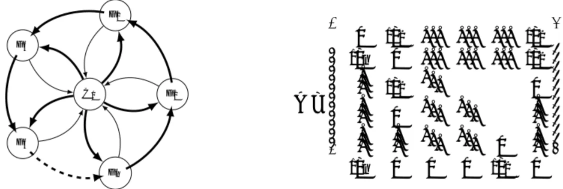
We consider the circular economy introduced in Figure 1 to highlight the effects at play when the initial impact of monetary shocks is heterogeneous. Within the circular economy the consumer assigns the same consumption budget to each firm and each firm uses a share1/2of
labor in its production process. Furthermore, each firm has a single supplier and a single buyer among firms. We assume the productivity parameter is such that ⁄i= 2 for each firm.
The household supplies n units of labor.
F1 F2 F3 F4 Fn C0 A= Q c c c c c c c c c c c a 0 1/2 . . . . 1/2 1/n 0 ... ... ... 1/2 ... 1/2 ... 0 ... 0 ... ... ... ... ... ... ... 0 ... 1/n 0 0 0 1/2 0 R d d d d d d d d d d d b
Figure 1: A circular economy with n firms, F1,···Fn and a consumer C0. The consumer
assigns the same consumption budget to each firm, each firm uses a share 1/2 of labor in
its production process, has a single supplier and a single buyer among firms. Links are directed from suppliers towards buyers. Thick lines correspond to weights of 1/2 thin lines
correspond to weights of 1/n.The matrix A is the adjacency matrix of the network where the
first line (resp. column) corresponds to the revenues (resp. expenses) of the household and the subsequent lines (resp. columns) to these of the firms.
In this framework, assuming total monetary mass is 3n, it is clear that at equilibrium all prices are equal to 1, each firm holds 2 units of working capital, produces 2 units of output using 1 unit of labor and 1 unit of input from its supplier whereas the household holds n units of wealth and consumes 1 unit of every good. That is, the equilibrium distribution of wealth, output and prices are given by the following table.
agent 0 1 2 3 ··· n
m n 2 2 2 2 2
q n 2 2 2 2 2
p 1 1 1 1 1 1
Suppose firm 1 receives a positive monetary shock of 2‘ > 0 at the end of period 0. The induced change in demand for firm 1 leads to the following state in stage 1.
agent 0 1 2 3 ··· n
m1 n 2 + 2‘ 2 2 2 2
q1 n 2 2 2 2 2
p1 1 +‘/n 1 1 +‘/2 1 1 1
Following the shock, firm 1 increases its demand to firm 2 and the household. This raises the price of labor and of firm 2’s output. For firm 1 the rise in labor price is more than compensated by its increase in working capital. Firm 1 thus increases its output. For the other firms the rise in the price of labor induces a decrease in output. The state at t = 2 is given by: agent 0 1 2 3 ··· n m2 n+ ‘ 2 2 + ‘ 2 2 2 q2 n 2 ˆ ı ı Ù (1 + ‘)2 (1 +‘/n)(1 +‘/2) 2 Û 1 1 +‘/n 2 Û 1 1 +‘/n 2 Û 1 1 +‘/n 2 Û 1 1 +‘/n p2 1 +‘/2n 2 +‘/n 2 ˆ ı ı Ù (1 + ‘)2 (1 +‘/n)(1 +‘/2) 2 +‘/n 2 Û 1 1 +‘/n 2 +‘/2+‘/n 2 Û 1 1 +‘/n 2 +‘/n 2 Û 1 1 +‘/n 2 +‘/n 2 Û 1 1 +‘/n m3 n+‘/2 2 +‘/n 2 +‘/n 2 +‘/2+‘/n 2 +‘/n 2 +‘/n
The increase in nominal demand triggered by the initial shock at this stage is mainly concentrated on firm 3 and on the household. This implies firm 3 has to increase price given output has not increased. Furthermore, the nominal demand faced by firm 1 is decoupled from the increase in its output. Therefore, firm 1 has to decrease its price. Thus a positive monetary shock can induce both increase and decrease of prices in the short-run.
To simplify analysis, we assume n is large and discard the terms‘/n. This simplifies the
expression of the state in stage 2 to:
agent 0 1 2 3 ··· n m2 n+ ‘ 2 2 + ‘ 2 2 2 q2 n 2 ˆ ı ı Ù(1 + ‘)2 (1 +‘/2) 2 2 2 2 p2 1 Û 1 +‘/2 (1 + ‘)2 1 1 +‘/4 1 1 m3 n+‘/2 2 2 2 +‘/2 2 2
The shock propagates further through two effects on production. Firm 2 increases its output because of the increase in nominal demand it faced. Firm n increases its output because of the decrease in the price of the input it buys from firm 1. This leads to the following state in stage 3 (neglecting terms of order ‘/n):
agent 0 1 2 3 4 ··· n m3 n+‘/2 2 2 2 +‘/2 2 2 2 q3 n 2 2 ˆ ı ı Ù(1 +‘/2)2 (1 +‘/4) 2 2 2 2( (1 + ‘)2 1 +‘/2 ) 1/4 p3 1 1 Û 1 +‘/4 (1 +‘/2)2 1 1 +‘/8 1 ( 1 +‘/2 (1 + ‘)2)1/4 m4 n+‘/4 2 2 2 2 +‘/4 2 2
As for firm 1 in stage 2, the increase of output by firms 2 and n is not matched by corresponding increase in demand. Both firms thus decrease prices.
In the following periods, the sequence of events “positive demand shock, increase of output, decrease in price, increase in output” propagates further. However, the size of the shock decays progressively each period as a part of the shock is absorbed by the household who redistributes demand uniformly among firms (through the term ‘/n neglected in our analysis).
Eventually, the shock is evenly distributed among firms generating a general rise in prices by a factor of 1 +2‘/3n.
3.2 Network structure and transmission of shocks
The above example shows that the impact of a monetary shock can be ambiguous in the short run. For example, a positive monetary shock can induce both increase and decrease in prices in the short run. The temporary volatility in prices generated by a monetary shock propagates across the network through two channels. One, a direct channel whereby the monetary shock induces a change in demand for inputs. Two, an indirect channel whereby firms respond to changes in the prices of inputs.
More generally, the short-term dynamics of prices is related to the network structure as follows. From equation 11, we have mt = At(m0+ ‘) = Atm0+ At‘= m0+ At‘. Using
Equation (13) we can completely characterize the dynamics of prices following a monetary shock by the structure of the supply network. First, for t = 2, for all i œ N :
log(p2i) = log(p0i) + log
A m3i m1i B + ÿ kœN Ak,ilog A m2k m0k B (19) = log(p0i) + log A m0i+ A3i,·‘ m0i+ Ai,·‘ B + ÿ kœN Ak,ilog Q am 0 k+ A2k,·‘ m0k R b (20)
Equation (20) suffices to illustrate the main drivers of price dynamics. The primitive cause of the variation of prices is the non-uniform speed of propagation of monetary shocks across the network. The shocks get propagated through walks of different lengths in the network and thus reach a given node with different lags. This implies firms might experience changes in the nominal demand they face as highlighted by terms of the form mtk+2/mt
k. The changes in nominal demand has a direct impact on prices corresponding to the term log1m3i/m1
i 2
in Equation (19). The direct channel induces a rate of change of prices that is proportional to the rate of change of nominal demands. This direct impact propagates upstream in the network: from buyers to sellers. The changes in nominal demand also has an indirect impact represented by the term qkœNAk,ilog
1
m2k/m0
k 2
, which corresponds to the feedback effect on
a firm from the changes in the prices of inputs induced by the direct demand effect. This indirect effect is mediated by the fact that changes in prices of the suppliers affects the production level of the firm and thus its price. The indirect effect propagates downstream in the network: from sellers to buyers.
given by: log(pt+1 i ) ≠log(p0i) = t≠1 ÿ ·=0 ÿ kœN A·k,ilog Q a m 0 k+ Atk,+2≠·· ‘ m0k+ ›{·<t}Atk,≠·· ‘ R b (21)
where › denotes the indicator function.
A linear expansion of this expression highlights the relative role of upstream and down-stream propagation mechanisms. Namely, denoting by log(pt) œ RN the column vector formed
by the log(pt
i) and by AÕ the transpose of A, one has:
Proposition 3. For small enough monetary shocks ‘, the dynamics of prices can be
approxi-mated as:
log(pt+1) ≠log(p0) = ÿt ·=0
(AÕ)·
mAt≠·(A2≠ I)‘ + (AÕ)t m‘ (22) where m is the diagonal matrix whose coefficients are the (m0k)kœN.
In line with the preceding discussion, equation (22) highlights the fact that the primitive driver of the dynamics is the volatility in nominal demand induced by the initial shock. This is represented by the term (A2≠ I)‘ corresponding to the differences between the direct impact
of the shock ‘ and its impact after a two period lag A2‘. The two period lag corresponds to
the difference between the time where production decisions are made and the time at which firms are confronted with demand. This lag in the propagation of shocks creates a mismatch between supply and demand which is resorbed by a deviation of prices from their equilibrium values. The size of this initial deviation (A2≠ I)‘ is determined by the local structure of the
network. More precisely, it depends on the incoming degree of order two i.e. the weights of incoming paths of length two. The initial price deviation is likely to be small if the network is homogeneous and the distribution of two-degrees is centred around average (equal to one). If a node has a large incoming degree of order two i.e. it is a large indirect supplier of the economy, it is likely to initially react in an unconventional manner to a monetary shock. For example, the firm may decrease its price following a positive monetary shock (indeed
A2i,·‘≠ ‘i is likely to be positive if ‘ œ RN+). Conversely, a node with small incoming degree of
order two is likely to initially exacerbate the effect of a monetary shock. This role of second order interconnectivity is reminiscent of the results in Acemoglu et al. (2012).
This initial volatility is then propagated in the network. The propagation is represented by the linear operator qt
·=0(AÕ)· mAt≠·. The operator corresponds to the combination of
upstream/forward and downstream/backward propagation channels identified above. The term At≠· corresponds to the upstream propagation of the variation of demand and of the
correlated variation of price from a firm to its suppliers. The term (AÕ)· corresponds to the
propagation of the feedback effect induced by the price variation of a firm on the price of its buyers through changes in production costs. Hence the term (AÕ)·At≠·(A2≠ I)‘ can be
interpreted as the propagation of the shock (A2≠ I)‘ for t ≠ · steps in the upstream/forward
direction and then for · steps in the downstream/backward direction. In other words, the shock propagates through demand effects for t ≠· steps via At≠· and through price effects
for · steps via (AÕ)·. More formally, (AÕ)·At≠· is the matrix of weights of walks of length
steps are in the opposite direction. The factor m corresponds to the scaling of the shock
proportionally to the initial monetary holdings. The operatorqt
·=0(AÕ)· mAt≠· corresponds
(up to the rescaling factor m) to the total weights of walks of length t in the network when
allowing for both forward and backward propagation. To sum up, the log-variation of price at the end of period t + 1, log(pt+1) ≠log(p0), corresponds to the propagation of the initial
shock (A2≠ I)‘ through the network in both forward and backward directions. The term
(AÕ)t
m‘ is a corrective term accounting for the fact that there is no variation of prices in
period 0 to be propagated backwards.
Remark 1. The propagation operator is very similar to the matrix of weights of walks
of length t upon which the computation of feedback centrality mesures is based (see e.g. Bonacich, 1987; Jackson, 2010). Explicitly, if one discards the rescaling factor m, one has
qt
·=0(AÕ)·At≠·= (A+AÕ)t, which corresponds to the matrix with the walks of length t for the adjacency matrix ˜A:= A + AÕ of the undirected network obtained by discarding the direction of links in A. Thus, up to the rescaling factor m, the cumulative logarithmic variation of prices at time T, VT :=qTt=0log(pt+1) ≠log(p0) is proportional to the sum of the Bonacich centrality, truncated at time T, of the undirected network ˜A with weights (A2≠ I)‘ and of the
original network A with weights ‘. (see Ballester et al., 2006).
It is worth noting that the transient variations in nominal demand at a node i following a shockmti+2/mt
i=(m
0
i+Atk,+2· ‘)/(m0i+Atk,·‘) are to a certain extent arbitrary. The transient changes
in demand are determined by the ratio between the weights of walks of different length leading from the sources of the shocks to the node under consideration. This ratio is determined by the structure of the network and can assume a wide range of value as discussed below (see proposition 4). A foremost consequence of this remark is that a given monetary shock can induce heterogeneous transient price response in different parts of the production network. In particular, a positive monetary shock could induce negative price change in the short-run. In what follows, we derive the behavior of the distribution of prices and the price-level in the course of the out-of-equilibrium propagation of monetary shocks.
3.3 The dynamics of the distribution of prices
At the micro-economic level, empirical evidence suggests monetary shocks generate wrong directional movement in some prices. For instance, Lastrapes (2006) and Balke and Wynne (2007) find about 50% of commodity prices change in the wrong direction in response to monetary shocks5. Our model provides an explanation of the wrong directional movement in
some prices.
Suppose a local positive shock induces an increase in the working capital of a firm i and consequently its demand for inputs from firm j. Firm j is likely to increase its price. However in so far as other buyers of firm j are not yet affected by the shock, the increase price may be less than the increase in demand by firm i. This allows firm i to purchase more inputs and increase output. Given the local nature of the shock, the increase in output may not be 5Balke and Wynne (2007) use data on monthly changes in the components of commodities Producer Price Index (PPI). At the highest level of disaggregation (the eight digit level) the data contains 130 time series in 1959 to 1228 time series in 2001. Lastrapes (2006) uses data of 69 commodity price indexes with complete monthly observations from 1959:1 to 2003:10.
matched by a corresponding rise in demand faced by firm i. And thus firm i may decrease its price next period. The price decrease induced by the intertemporal gap between supply and demand faced by firms propagates upstream through the supply chain, i.e. it affects the suppliers of the firm with a delay. Firm i’s price decrease creates a second source of potential price anomalies: following the price decrease, the buyers of firm i can increase their output. The process can lead to further decrease in prices if the increased output is not matched by a corresponding increase in demand. This effect propagates downstream in the supply chain: from a firm to its buyers. These price anomalies progressively disappear as the initial monetary shock diffuses in the network. Over time the increase in nominal demand becomes uniform and is matched by a corresponding general rise in prices. In the long-run the quantitative theory of money holds. As emphasized in propositions 1 and 3, the magnitude and the duration of the price anomalies are determined by the structure of the network and the characteristics of the initial shock. At the micro-economic level, the variations induced by the shock can be arbitrary. Namely, one has:
Proposition 4. For every finite sequence of prices p = (p0, p1,··· ,pT) œ RT++1 such that p1Ø p0, there exists a network economy E(1,⁄), a monetary shock ‘ œ RN and a firm i such that the sequence of prices of firm i in the T first periods is p.
More broadly, according to Proposition 3, the dynamics of the price distribution is completely determined by the structure of the network.
3.4 The Price Puzzle
Numerous econometricians have reported a short run increase in the price level in response to monetary contractions (see e.g. Hanson, 2004; Rusnak et al., 2013, and references therein). Our model generates a rise in the price level if monetary contractions disproportionately affect the suppliers of consumer goods but are transmitted to consumer’s final demand with a lag. Under these two conditions, in the short run the supply of consumer goods decreases more than the final demand thereby generating an increase in the prices of consumer goods. In what follows, we characterize a general class of “supply-chain” economies which generate an increase in the price level following a contractionary monetary shock.
We define a supply-chain economy as a network economy E(A,⁄) together with a set of L layers: {L1,··· ,LL}. The set of layers form a partition of the set of firms M. A firm in layer ¸
has all its suppliers in layer ¸≠1 and all its consumers in layers ¸+1 (among firms). In other words, the adjacency matrix (restricted to firms) of the economy is upper triangular by block. This structure is very similar to the one considered in early contributions investigating the propagation of shocks in production networks (Bak et al., 1993; Scheinkman and Woodford, 1994; Battiston et al., 2007). We assume the household consumes goods produced by firms in layer L. The household’s supply of labor is normalized to 1. Let k denote the share of labor supplied to layer L at equilibrium. Assuming without loss of generality that the total wealth is such that the price of labor is normalized to 1, one has:
k= ÿ iœLL a0,im0i and (1 ≠k) = ÿ jœL≠L a0,jm0j (23)
In this setting, suppose all firms in layer L are affected by an homogeneous negative monetary shock of magnitude fl: the working capital of each firm i in layer L decreases to (1 ≠fl)m0
i.One has:
Proposition 5. Assume the share of labor supplied to layer L at equilibrium is k and that
there is an homogeneous negative monetary shock of magnitude fl on the firms of layer L, then the price of firms of layer L in period 2 is given by:
p2i =(1 ≠flk) a0,i+1
(1 ≠fl)a0,i pi,0. (24)
Corollary 2. Under the conditions of proposition 5, for k sufficiently small, following a
negative monetary shock, all consumer prices (i.e. all prices in layer L) increase in the short run (i.e. in period 2).
Under Corollary 2 a negative monetary shock induces a short-term increase (at least in period 2) of the price level. Two conditions are sufficient for a rise in the price level in response to monetary contractions to emerge in the network economy. First, the shock must be sufficiently downstream (in layer L). This condition ensures a monetary contraction generates a decrease in the supply of consumer goods. Second, firms initially affected by the monetary contraction must bear a sufficiently low proportion of the economy’s wage bill (k must be small enough). This condition ensures that the monetary contraction takes sufficiently long time to generate the full long run decrease in final demand. The two conditions jointly guarantee that in the short run supply decreases more than final demand, thereby generating an increase in the price-level in response to monetary contractions. The lower the share k of downstream firms in the wage bill, the larger the discrepancy between the variations of final supply and demand for consumer goods. And thus the more pronounced the rise in the price level after a monetary contraction as highlighted in Equation 24.
4
Empirical validation of the model
4.1 Small firms in the US economy
A first empirical test of our model is to investigate whether the sufficient conditions put forward in Proposition 5 and Corollary 2 for the emergence of the price puzzle are empirically satisfied. Thus, we empirically investigate two issues. First, whether downstream firms are disproportionally affected by monetary contractions. And second what is the relative share of downstream firms in the wage bill of the US economy.
With respect to the first issue, no one has so far empirically examined the relation between the impact of monetary shock upon a firm and its position in the production network. However, converging empirical and theoretical evidence suggests small firms are disproportionally affected by monetary shocks6. Therefore, if small firms are highly represented
6For empirical evidence see Gertler and Gilchrist (1994); Gaiotti and Generale (2002); Iyer et al. (2013); Carb´o-Valverde et al. (2016). For theoretical models see Greenwald and Stiglitz (1993); Holmstrom and Tirole (1997); Clementi and Hopenhayn (2006)
downstream, then downstream firms will be more hurt by monetary contractions. We assess the validity of the first condition by analyzing the share of small firms in downstream sectors. The Small Business Administration (SBA) provides sectoral data on the size (by sales receipts) distribution of firms in the U.S7. In order to measure the relative share of small firms in
downstream sectors, we match the SBA data to Bureau of Economic Analysis’s data on the sectoral composition of personal consumption expenditure (PCE)8. Firms with annual
revenues of less than a million USD account for 11.6% of the sales of basket of goods used to compute the PCE. The share of firms with annual revenues of less than a million USD in economy wide sales is 4.4%. Hence, small firms are disproportionately highly represented among the producers of consumer goods. Such a pattern is also visible in more aggregate data. Small firms play a minor role in sectors like mining and manufacturing which do not appear in the basket of consumer goods. For instance, firms with annual receipts of less than a million USD account for about 20% the output of Services, while their share in Manufacturing, Mining, and Utilities is less than 2%. Figure 2 presents a direct measure of the over representation of small firms in the basket of goods which enter the Personal Consumption Expenditure Index (PCE) in 305 sectors. The x-axis of Figure 2 measure the share of firms with yearly receipts of less than one million in the total receipts of a sector. The y-axis measure the ratio of the share of a sector in PCE to its share in the economy. The y-axis therefore captures the disproportional representation of a sector in the PCE. The correlation coefficient between the two variables is 0.09 and Spearman’s rank correlation is 0.14. And a robust OLS line has a slope of 0.11. The positive relation between the variables in Figure 2 suggests sectors with a high share of small firms have a disproportionately high representation in the PCE.
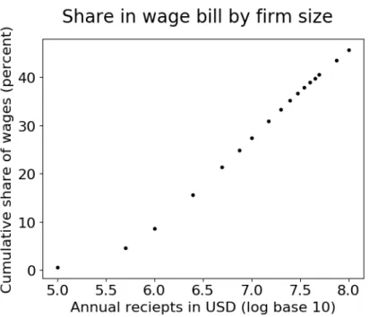
With respect to the second issue, we study the share of small firms in the wage bill of the economy using data from the Small Business Administration. Figure 3 presents the relation between size of firms and their share in the economy’s wage bill. The y-axis presents cumulative share in wages. The x-axis present annual receipts. Figure 3 shows that small firms do not account for the majority of the wages in the US economy.
7Of the 1095 sectors for which SBA provides data, 644 are at the NAICS six digit level, 378 at the five digit level, 72 at the four digit level, and 1 at the three digit level. All sectors are represented at the highest digit level for which firm size distribution data is available
8We match sectors using the NAICS-BEA codes mapping provided by the BEA. Not all the sectoral classification of the Input-Output are at the same NAICS digit level as the SBA size distribution. Exact matching of NAICS codes accounts for about 78% of PCE, whereas fuzzing matching accounts for more than 99% of PCE. Fuzzy matching of NAICS follows the simple rule of matching unmatched NAICS codes from the Input-Output table with up to 1-3 digit higher level codes.
Figure 2: The plot marks 305 sectors. The x-axis is the log of the share of firms with receipts of less than one million in the total receipts of a sector. The y-axis is the log of the ratio of a sectors share in the Personal Consumption Expenditure to its share in the economy. The shares are computed using the Input-Output table. The slope of the line in the plot is 0.105 and the intercept is -0.121. The slope and intercept are computed using robust OLS.
Figure 3: The plot marks the share of firms with different sizes in the wage bill of the economy. The y-axis is the cumulative wage bill. The x-axis is the log of the annual receipts with 17 different sizes.
4.2 Computational experiments on the U.S. production network
Section 3 illustrates the emergence of an increase in the price level in response to a monetary contraction within a stylised setting. In this section, we investigate the empirical relevance of our model by calibrating it to granular data on the US production network. Furthermore, we extend the model to study the consequences of a more general distribution of monetary shocks. Rather than assuming the initial impact of monetary shock falls upon firms in specific parts of the network, we allow all firms to bear the initial impact of monetary shocks albeit to different degrees. The magnitude of the initial impact of a monetary shock is inversely correlated to the size of the firm.
4.2.1 US firm network data
We use firm-level data from S&P Capital IQ and Orbis BvD datasets to calibrate our model. Our data set includes 105,940 buyer-seller relationships between 51,913 firms for whom we have revenue information and NAICS codes9. While the coverage of our data set is sparse
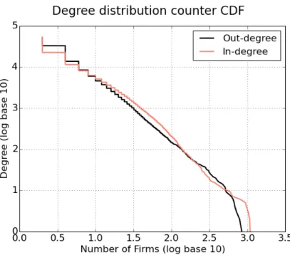
compared to the universe of US firms, it is nevertheless the most comprehensive dataset on supply relationships between US firms currently available. Our data set contains both private and publicly listed firms whereas datasets used in previous studies on production networks are limited to only contain listed firms (Atalay et al., 2011; Wu and Birge, 2014) or aggregated input-output network (Acemoglu et al., 2012). The inclusion of a subset of non-listed firms is relevant given the role of small firms in our explanation of the price puzzle. Figure 4 shows our data set matches the stylized fact that the degree distribution of the production network follows a power-law (Atalay et al., 2011; Konno, 2009). And Figure 5 shows the mid portion revenue distribution of the firms in our data set follows a power-law like the revenue distribution of the universe of firms in the US (Axtell, 2001).
9S&P Capital IQ has a rich database about supply relationships between US firms from 2005 to 2017. We restricted the universe of firms to private firms and publicly listed firms. We excluded banks, non-banking financial corporations, and government entities. These restrictions left us with data on the business relationships between 80,092 US firms. Of the 80,092 firms Capital IQ provided data on revenues and NAICS sector codes for 43,321 firms. We used Orbis BvD to gather data on revenues or NAICS codes for 8,592 of the 36,771 firms with missing data. Completing the Capital IQ data set with information from Orbis BvD yielded a total of 105,940 supply relations between 51,913 firms for whom we know revenues and NAICS sectoral codes.
Figure 4: Degree distribution counter CDF.
Figure 5: Annual revenues.
4.2.2 The computational experiments
We calibrate the model to US firms production network by assigning the matrix of observed supply relationships as the adjacency matrix of the network. This matrix is however un-weighted (as Capital IQ does not collect the corresponding information). We use a taylored
algorithm to calibrate the weights in such a way that the empirical distribution of revenues for the firms is an invariant distribution of Equation 1410. We also calibrate the network economy
so that the households spending on different firms in our data set matches the sectoral distribution of household personal consumption expenditure (PCE) in the Input-Output table. We then set the initial value of prices, money holdings, and stocks of output to their equilibrium values. The system is initialized in the steady state—in the sense of Proposition 2—corresponding to empirical observations about revenues and supply relationships.
We then run a series of computational experiments to investigate the dynamic response of prices following a monetary shock. In these experiments, each time step of the model is interpreted as a quarter on the basis of empirical observations about the frequency of price changes. Blinder (1991) for instance finds firms change prices in response to changes in cost and demand with the delay of a quarter. The monetary shocks considered in our experiments are constructed as follows. A first parameter s œ [0,1] measures the aggregate size of the shock. A second parameter ◊ œ R+ measures the heterogeneity of the shock
with respect to firms’ sizes. Let M =qiœNmi denote the total money in circulation in the
economy. A monetary contraction of size s removes sM units of money from circulation. A monetary contraction is implemented through a reduction in the working capital of each firm
iproportional to m◊i. We focus on the case where ◊ < 1 when small firms are disproportionally
affected by monetary contractions. The case ◊ > 1 would correspond to large firms being disproportionally affected by the contraction. While the case ◊ = 1 corresponds to the case where firms are homogeneously affected by the shock and prices instantaneously adjust to their new equilibrium value (see Corollary 1).
We run series of computational experiments with variation in the size s of the monetary shock and the heterogeneity ◊ of the initial impact of the shock. We focus on the dynamics of the price level measured using weights of the Personal Consumption Expenditure (PCE) from the Input-Output Table11. The figures below summarise data from about 500 computational
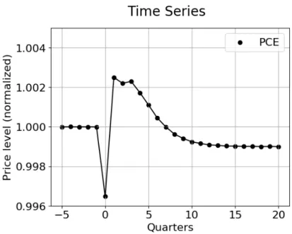
experiments on the calibrated US economy with more than a million firm interactions. Figure 6 highlights a typical response of the system following a shock in that case. In the first time step after a monetary contraction, some prices decreases and no prices rise. As discussed in Section 3, in the first time step after a monetary contraction some firms experience a decrease in the demand for their goods because their buyers experienced a decrease in working capital. The firms which experience a decrease in demand decrease the prices of their goods. From the second time periods onward, the percolation of monetary shocks generates an increase in the price level because the short term contraction in the supply of consumer goods is more than the decrease in nominal final demand. The price level is greater than the pre-shock level from the second to the seventh quarter after the monetary contraction. The initial increase in the price level is of the same order of magnitude as the long run decrease. The wrong directional change in the price level generated by our model is on the same order of magnitude as that which is reported by several empirical studies Rusnak 10Estimating the network weights so that given firm sizes are the invariant distribution is a large matrix quadratic programming problem. We solved the problem using IBM’s CPlex software.
11The price level is computed in the following manner. The sectoral weights of the Personal Consumption Expenditure Index (PCE) are obtained from the Input-Output Table. The total weights of firms of a given sector in the price level is set equal to the share of that sector in the PCE. The total weight of a given sector is equally divided among firms in that sector within our data set.
et al. (2013). It is worth noting that empirical studies on the Price Puzzle do not document an initial decrease in the price level, which is a point of difference with respect to the results generated by our model. One potential reasons for this difference is the synchronous setting of prices within our model. Real world pricing decisions are asynchronous. Within asynchronous pricing, the first price change of different firms in response to a monetary contraction will not occur at the same time step. Therefore, the price level may not decrease in the first quarter after a monetary contraction because some firms are into their second or greater rounds of price change, while others are yet to change their prices.
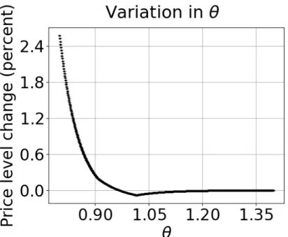
An increase in the price level after monetary contractions systematically occurs when small firms are disproportionally affected by monetary contractions for sufficiently low value of ◊. The presence of the price puzzle is robust to changes in the magnitude s and the heterogeneity of the shock ◊ (for a sufficiently low value of ◊). Figure 7 illustrates the sensitivity of the model with respect to the strength of the monetary shock by showing the relation between the size of the monetary contraction (that is measured indirectly by the long-run change in the price level) and the size of the short-run change of the price level in the opposite direction. The y-axis in Figures 7 and 8 measure the percent change between the pre-shock price level and the maximum price level in six quarters after a monetary contraction. Figure 7 shows that the wrong directional change in the price level is of the same order of magnitude as the long-term effect of the monetary contraction. Figure 8 illustrates the sensitivity of the price level response with regards to the heterogeneity of the impacts. The response is non-linear12.
The size of the price puzzle increases rapidly with the heterogeneity in initial impact of monetary shocks (|1≠◊|). This highlights the importance of the correlation between network structure and firm size in the propagation of monetary shocks.
12Note that in Figure 8 a monetary contraction of size s = ≠0.001 does not cause a temporary increase in the price level in the calibrated economy when ◊ > 0.97. This is simply because when ◊ is sufficiently high the decrease is supply of consumer goods is overwhelmed by the short run decrease in the nominal demand for consumer goods for the given size of monetary contraction. The exact value of ◊ beyond which monetary contractions will not generate an increase in the price level will depend on the size of the contraction and the size distribution of firms within the production network.
Figure 6: Price response to a negative monetary shock of size s = ≠0.001., ◊ = 0.9.
Figure 7: Long-run versus short-run changes in the price level for ◊ = 0.95. The x-axis corresponds to the size of the long-run (negative) price level change or equivalently to the size s of the monetary shock. The y-axis measured the (positive) change in prices the first quarter after a monetary contraction.