Objective evaluation of surface-and satellite-driven carbon dioxide atmospheric inversions

(1)

HAL Id: hal-02862570

https://hal.archives-ouvertes.fr/hal-02862570

Submitted on 9 Jun 2020

HAL is a multi-disciplinary open access

archive for the deposit and dissemination of

sci-entific research documents, whether they are

pub-lished or not. The documents may come from

teaching and research institutions in France or

abroad, or from public or private research centers.

L’archive ouverte pluridisciplinaire HAL, est

destinée au dépôt et à la diffusion de documents

scientifiques de niveau recherche, publiés ou non,

émanant des établissements d’enseignement et de

recherche français ou étrangers, des laboratoires

publics ou privés.

carbon dioxide atmospheric inversions

Frederic Chevallier, Marine Remaud, Chris W. O’dell, David Baker, Philippe

Peylin, Anne Cozic

To cite this version:

Frederic Chevallier, Marine Remaud, Chris W. O’dell, David Baker, Philippe Peylin, et al..

Objec-tive evaluation of surface-and satellite-driven carbon dioxide atmospheric inversions. Atmospheric

Chemistry and Physics, European Geosciences Union, 2019, 19 (22), pp.14233 - 14251.

�10.5194/acp-19-14233-2019�. �hal-02862570�

(2)

https://doi.org/10.5194/acp-19-14233-2019 © Author(s) 2019. This work is distributed under the Creative Commons Attribution 4.0 License.

Objective evaluation of surface- and satellite-driven carbon dioxide

atmospheric inversions

Frédéric Chevallier1, Marine Remaud1, Christopher W. O’Dell2, David Baker2, Philippe Peylin1, and Anne Cozic1

1_{Laboratoire des Sciences du Climat et de l’Environnement, LSCE/IPSL, CEA-CNRS-UVSQ, Université Paris-Saclay,}

91198 Gif-sur-Yvette, France

2_{Cooperative Institute for Research in the Atmosphere, Colorado State University, Fort Collins, CO, USA}

Correspondence: Frédéric Chevallier ([email protected]) Received: 4 March 2019 – Discussion started: 15 April 2019

Revised: 28 September 2019 – Accepted: 10 October 2019 – Published: 26 November 2019

Abstract. We study an ensemble of six multi-year global Bayesian carbon dioxide (CO2) atmospheric inversions that

vary in terms of assimilated observations (either column re-trievals from one of two satellites or surface air sample mea-surements) and transport model. The time series of inferred annual fluxes are first compared with each other at various spatial scales. We then objectively evaluate the small inver-sion ensemble based on a large dataset of accurate aircraft measurements in the free troposphere over the globe, which are independent of all assimilated data. The measured vari-ables are connected with the inferred fluxes through mass-conserving transport in the global atmosphere and are part of the inversion results. Large-scale annual fluxes estimated from the bias-corrected land retrievals of the second Orbiting Carbon Observatory (OCO-2) differ greatly from the prior fluxes, but are similar to the fluxes estimated from the surface network within the uncertainty of these surface-based esti-mates. The OCO-2-based and surface-based inversions have similar performance when projected in the space of the air-craft data, but the relative strengths and weaknesses of the two flux estimates vary within the northern and tropical parts of the continents. The verification data also suggest that the more complex and more recent transport model does not im-prove the inversion skill. In contrast, the inversion using bias-corrected retrievals from the Greenhouse Gases Observing Satellite (GOSAT) or, to a larger extent, a non-Bayesian in-version that simply adjusts a recent bottom-up flux estimate with the annual growth rate diagnosed from marine surface measurements both estimate much different fluxes and fit the aircraft data less. Our study highlights a way to rate global atmospheric inversions. Without any general claim regarding

the usefulness of all OCO-2 retrieval datasets vs. all GOSAT retrieval datasets, it still suggests that some satellite retrievals can now provide inversion results that are, despite their un-certainty, comparable with respect to credibility to traditional inversions using the accurate but sparse surface network and that are therefore complementary for studies of the global carbon budget.

1 Introduction

Carbon dioxide (CO2) is increasingly monitored in the global

atmosphere due to its important role in climate change. For example, NOAA’s GLOBALVIEWplus Observation Pack-age (ObsPack, Cooperative Global Atmospheric Data Inte-gration Project, 2018) archives high-quality measurements made at the surface or from aircraft by various institutes. De-spite occasional budget difficulties (Houweling et al., 2012), the number of collected data points has exponentially in-creased over the years, with, in reference to 1980, 6 times more measurements in 2000 and 100 times more measure-ments in 2017. In addition, the ground-based Total Carbon Column Observing Network of column retrievals (TCCON, Wunch et al., 2011) is less than 15 years old but already op-erates about 30 sites over the globe. Other measurements, like the recent AirCore technique that samples air in free-fall tubes (Karion et al., 2010) or the COllaborative Carbon Column Observing Network (COCCON, Frey et al., 2019), have also emerged in the past decade. Most remarkably, the number of spectrometers designed to monitor the CO2

(3)

of 2018 (CEOS Atmospheric Composition Virtual Constella-tion Greenhouse Gas Team, 2018). The primary motivaConstella-tion for this increase in CO2observations has been to further our

understanding of the global surface fluxes of carbon, with the additional help of meteorological data (e.g. Bolin and Keel-ing, 1963; WMO, 2018). This is done in practice by inversion of atmospheric transport models within a Bayesian frame-work (e.g. Peylin et al., 2013). Scientists have urged caution when interpreting this growing amount of data because the uncertainty of the available meteorological information was identified early as a critical limitation on the exploitable mea-surement information. This limitation motivated the creation of the international Atmospheric Tracer Transport Model In-tercomparison project 25 years ago (TransCom, Law et al., 1996) and is still relevant today (Schuh et al., 2019). Ade-quate representation of the various error statistics involved in the Bayesian estimation remains a challenge (e.g. Boc-quet et al., 2011). In addition, column retrievals, made from measured radiances from space or on the ground after com-plex processing, cannot fundamentally be calibrated relative to WMO-traceable standards, in contrast to surface measure-ments like those in ObsPack GLOBALVIEWplus. Indeed, systematic errors in the retrievals at the sub-micromole per mole level (10−6mol mol−1, abbreviated as part per million, ppm) are enough to affect the flux estimation (Chevallier et al., 2007), but the current TCCON retrievals that serve as the best reference for column retrievals with global coverage have site-specific commensurate offset uncertainties (Wunch et al., 2015).

A given inversion configuration is made of one or sev-eral observation types, a transport model and a few statistical models. Many of them seem reasonable. Although model dis-agreement has been reduced over the last couple of decades, current inversion results show an unacceptably large spread, even for zonal averages (e.g. Le Quéré et al., 2018). This study aims at evaluating whether simple measures of qual-ity based on airborne measurements in the free troposphere can distinguish between six inversion configurations. These inversion configurations differ in the assimilated data and in the transport model. The assimilated data are either surface measurements in ObsPack and related databases, retrievals from the Greenhouse Gases Observing Satellite (GOSAT) or the second Orbiting Carbon Observatory (OCO-2). The transport models are two versions of the atmospheric gen-eral circulation model of the Laboratoire de Météorologie Dynamique (LMDz, Hourdin et al., 2013) nudged towards analysed meteorological variables. The Bayesian inversion system from the Copernicus Atmosphere Monitoring Ser-vice (CAMS, https://atmosphere.copernicus.eu/, last access: 21 November 2019, Chevallier et al., 2005) is used in all six inversions. We use a “poor man’s inversion” (Chevallier et al., 2009) based on recent bottom-up fluxes and on the global annual atmospheric growth rate estimated from the average of marine surface measurements (Conway et al., 2014) to de-fine a baseline for the skill of each Bayesian inversion result.

Our use of airborne measurements in the free troposphere as verification data is motivated by their frequent, WMO-traceable calibration, their independence from all data as-similated here (including the measurements in the boundary layer) and their spatial distribution that samples all oceans and continents. Arguably they are the only CO2dataset that

possesses all three of these qualities.

In the following, data and models are described in Sect. 2, while Sect. 3 presents the various results. The results are dis-cussed in Sect. 4, and Section 5 concludes the study.

2 Model, system and data 2.1 Transport models

LMDz is the atmospheric component of the Earth system model of the Institut Pierre-Simon-Laplace (Dufresne et al., 2013) which has been contributing to the recent versions of the Climate Model Intercomparison Project (CMIP) estab-lished by the World Climate Research Programme (https:// www.wcrp-climate.org/wgcm-cmip, last access: 21 Novem-ber 2019). Here, we use its offline version (Hourdin et al., 2006) to simulate the transport of CO2. The offline

LMDz model reads a frozen archive of 3-hourly mean me-teorological data pre-computed by the full LMDz so that it only needs to simulate large-scale advection and sub-grid transport processes (i.e. deep convection and boundary layer turbulence). LMDz is nudged towards 6-hourly anal-ysed meteorological variables, here either ERA-Interim (Dee et al., 2011) or ERA5 (https://www.ecmwf.int/en/forecasts/ datasets/archive-datasets/reanalysis-datasets/era5, last ac-cess: 31 January 2019) with a relaxation time of 3 h. Online and offline models are consistently run at the same spatial resolution in order to avoid any challenging interpolation of the air mass fluxes for the sub-grid processes (see e.g. Yu et al., 2018): here 39 eta-pressure layers between the surface and around 80 km above sea level (km a.s.l.), and 96 grid points × 96 grid points, i.e. a horizontal resolution of 1.89 in latitude × 3.75◦ in longitude. This configuration discretises the 2–7 km a.s.l. region of the atmosphere, which will be a major focus in the following, into 6 to 10 layers, depending on local orography.

We use two physical formulations of LMDz, called 5A (in code identification number 1649) and 6A (in code identifica-tion number 3353), as described by Remaud et al. (2018, and references therein). The gap between the two versions rep-resents about 6 years of development from the LMDz team and includes e.g. a complete revision of radiation, the intro-duction of the thermodynamical effect of ice and changes in the sub-grid-scale parameterisations (convection, boundary layer dynamics) and in the land surface processes. For ver-sion 5A, horizontal winds are nudged towards ERA-Interim, but we use the new ERA5 for LMDz6A. Therefore, the dif-ferences between the two versions cannot be exclusively

(4)

at-tributed to sub-grid-scale processes, as boundary variables (nudging files and land processes) differ as well.

2.2 Inversion system

LMDz is embedded within the CAMS CO2inversion system.

This system minimises a Bayesian cost function to optimise the grid cell 8-day surface fluxes (with a distinction between local night-time fluxes and daytime fluxes, but without fos-sil fuel emissions, which are prescribed) and the initial state of CO2. To do so, it assimilates a series of CO2

observa-tions over a given time window within the LMDz model. The minimisation approach is called “variational” because it explicitly computes the gradient of the cost function us-ing the adjoint code of LMDz. Prior information about the surface fluxes is provided to the Bayesian system by a com-bination of climatologies and other types of measurement-driven flux estimates (e.g. Emission Database for Global At-mospheric Research version 4.3.2, Crippa et al., 2016, scaled globally and annually from Le Quéré et al., 2018, for the fos-sil fuel emissions or Landschützer et al., 2017, for the ocean fluxes). Details can be found in Chevallier (2018a). Of spe-cial interest here is the fact that, when integrated over a cal-endar year, prior natural fluxes are zero over all land grid points: this implies that the interannual variability of the in-ferred annual mean of terrestrial vegetation fluxes is gener-ated by the assimilgener-ated observations only. Over a full year, the total 1σ uncertainty (resulting from assigned error vari-ances that vary in space and time, and from assigned tempo-ral and spatial error correlations) for these prior land fluxes amounts to about 3.0 GtC a−1. The error statistics for the open ocean correspond to a global air–sea flux uncertainty of about 0.5 GtC a−1.

The assimilation window is either 19 years for the surface measurements (from January 2000 to October 2018), 8 years for the GOSAT retrievals (from January 2009 to Decem-ber 2016) or 4 years for the OCO-2 retrievals (from Septem-ber 2014 to July 2018).

2.3 Assimilated observations

All assimilated observations are the dry air mole fraction of CO2.

Assimilated surface air sample measurements have been selected from four large ongoing databases of atmospheric CO2 measurements: (i) NOAA’s ObsPack (Cooperative

Global Atmospheric Data Integration Project, 2018, and Car-bonTracker Team, 2018), (ii) the World Data Centre for Greenhouse Gases archive (WDCGG, https://gaw.kishou.go. jp/, last access: 21 November 2019), (iii) the Réseau Atmo-sphérique de Mesure des Composés à Effet de Serre database (RAMCES, http://www.lsce.ipsl.fr/, last access: 21 Novem-ber 2019) and (iv) the Integrated Carbon Observation System Atmospheric Thematic Centre (ICOS-ATC, https://icos-atc. lsce.ipsl.fr/, last access: 21 November 2019). The list of

se-lected sites and maps of their location are given by Cheval-lier (2018a). Each dataset provides at least 5 years of mea-surements. The error variances assigned to these measure-ments in the inversion system correspond to transport mod-elling uncertainty (analytical measurement uncertainty of in situ CO2data is a negligible component) and are computed

as the variance of the high-frequency variability of the de-seasonalised and de-trended CO2 time series of the daily

mean measurements at each site. These variances are then in-flated in order to give the same weight to each measurement day at a given location.

GOSAT was launched in January 2009, as a joint project of the Japan Aerospace Exploration Agency (JAXA), the Na-tional Institute of Environmental Studies (NIES) and Japan’s Ministry of the Environment (MOE) (Kuze et al., 2009). OCO-2 is a NASA satellite that was launched in July 2014 (Eldering et al., 2017). Both satellites still collect scientific data today. They orbit around the Earth from pole to pole with a local crossing time at the Equator in the early local af-ternoon. Each carries a spectrometer that measures the sun-light reflected by the Earth and its atmosphere in the near-infrared/shortwave infrared spectral regions, with high spec-tral resolution (>∼ 20 000) such that individual gas absorp-tion lines are resolved. OCO-2 provides spatially dense data with a narrow swath and with footprints of a few square kilo-metres, whereas GOSAT provides coarser-resolution data (100 km2 at nadir) with low spatial density. Various algo-rithms have been developed to retrieve the column-average dry air mole fraction of CO2 in the atmosphere (XCO2)

from the measured radiance spectrums. For GOSAT, we use bias-corrected XCO2retrievals from the OCO Full Physics

(OCFP) v7.1 product made by the University of Leicester and available from the Copernicus Climate Change Service for the period from April 2009 to December 2016 (https: //climate.copernicus.eu/, last access: 21 November 2019). For OCO-2, we use NASA’s Atmospheric CO2Observations

from Space (ACOS) bias-corrected retrievals, version 9 (Kiel et al., 2019; O’Dell et al., 2018) from September 2014 to July 2018. In both cases, a previous release of the CAMS surface-based inversion contributed to the retrieval official bias-correction to some extent. We neglect this dependency in the following because other reference data are used that re-duce the weight of the CAMS inversion (e.g. TCCON), and because the bias-correction schemes rely on two to five time-and space- invariant parameters only, with internal retrieval variables (e.g. the retrieved vertical CO2 gradient between

the surface and the free troposphere) as predictors. We do not tune the official retrieval bias corrections. To reduce data volume without loss of information at the scale of a global model, glint and nadir OCO-2 retrievals have been averaged in 10 s bins for the Model Intercomparison Project (MIP) of OCO-2, as described in Crowell et al. (2019), and we use them in this form. The retrieval averaging kernels, prior pro-files and Bayesian uncertainty are accounted for in the assim-ilation of both types of satellite retrievals (the interpolation

(5)

procedure between the model vertical grid and the retrieval grid is described in Sect. 2.2 of Chevallier, 2015). For OCO-2 retrievals, we also use the transport uncertainty term that is provided by the OCO-2 MIP, based on the variability across several models at the OCO-2 sounding locations (Crowell et al., 2019).

Maps of the coverage of GOSAT and OCO-2 retrievals are shown in Bösch and Anand (2017) and O’Dell et al. (2018), respectively. We only consider “good” retrievals as identi-fied by the xco2_quality_flag variable of each product. Both land and ocean data are used for GOSAT. GOSAT data over ocean have matured in the ∼ 10 years since they were first produced, and have reached a point where they appear to have smaller biases than over land (Zhou et al., 2016). Their direct inclusion in inversions also appears to be beneficial (Deng et al., 2016). However, although the ocean biases in OCO-2 have been substantially reduced since the initial ver-sion 7 (O’Dell et al., 2018), initial inverver-sion tests using OCO-2 ocean observations still produced highly unrealistic results (annual global ocean sinks of about 5 GtC a−1compared with the much smaller state-of-the-art estimates in Le Quéré et al., 2018) and are therefore left out of this work (as are retrievals over inland water or over mixed land–water surfaces). As for GOSAT, this situation may change in time and OCO-2 ocean data could be beneficial in future inversion set-ups. Despite the exclusion of ocean retrievals and the 10 s averaging, there are still 65 % more OCO-2 retrievals than GOSAT retrievals assimilated on average per month.

2.4 Verification observations

We use some specific measurements of the dry air mole frac-tion of CO2 as verification data. They are aircraft

measure-ments in the free troposphere made between July 2009 and December 2017 and archived in different ObsPacks (Coop-erative Global Atmospheric Data Integration Project, 2018, and NOAA Carbon Cycle Group ObsPack Team, 2018). Ta-ble 1 lists the various aircraft measurement sites, campaigns or programmes. For simplicity, all sites, campaigns or pro-grammes will be referred to as “propro-grammes” in the fol-lowing. All measurements have been calibrated to the WMO CO2X2007 scale or to the NIES 09 CO2scale to better than

0.1 ppm (e.g. Machida et al., 2008; Sweeney et al., 2015). We note that no aircraft data are assimilated here (Sect. 2.3).

We define the free troposphere as the altitudes between 2 and 7 km a.s.l. We avoid data below 2 km because (i) local anthropogenic emissions affect many aircraft measurements there, and (ii) some of the aircraft flew in the vicinity of mea-surement sites that have been used in the surface-based inver-sions. We avoid data above 7 km because the measurement variations (and the flux regional signal) are much reduced there. A few outliers for which the difference between model and observation is larger than 40 ppm are rejected: they likely represent very local pollution plumes.

Figure 1. Location of the aircraft measurements used in the free tro-posphere for the two verification periods. Note that the two periods overlap by 22 months, so that many data appear on both maps.

We define two periods for the following statistical com-putations. They are based on the availability of the satel-lite retrievals and of the aircraft data in the databases used here: a “GOSAT period” from July 2009 to September 2016 and an “OCO-2 period” from December 2014 to Decem-ber 2017. Note that they overlap and that there is a minimum of 3 months between the temporal bounds of the verification data and the temporal bounds of the assimilated data in or-der to account for inversion spin-up and spin-down. Figure 1 shows the geographical location of the verification data for the two periods.

2.5 Poor man’s inversion

In order to put the differences between inversion simulations and aircraft measurements into perspective, we compare them to an inversion that only assimilated the annual global growth rate of CO2. This baseline, called “the poor man’s

inversion” by Chevallier et al. (2009), adjusts prior natural fluxes over land in order to fit the annual trend of glob-ally averaged marine measurements (http://www.esrl.noaa. gov/gmd/ccgg/trends/, last access: 10 January 2019) multi-plied by a conversion factor (2.086 GtC ppm−1, from Prather, 2012) when combined with prior ocean and fossil fuel fluxes. The correction to the natural land fluxes is made proportional to the prior error standard deviations assigned within a given inversion system. In the case of the CAMS system here, the prior error standard deviations are themselves proportional to a climatology of heterotrophic respiration fluxes simulated by a vegetation model, with a ceiling of 4 gC m−2d−1. This simple approach is not Bayesian because prior error corre-lations are ignored, but it still allows transport models to fit

(6)

Table 1. Aircraft measurement programmes used here. Note that the ALF, PAN, RBA-B, SAN and TEF programmes are gathered under the identifier “INPE” (for Instituto Nacional de Pesquisas Espaciais) in Fig. 8.

Measurement programme identifier in ObsPack

Measurement programme name Specific doi Data providers

AAO Airborne Aerosol Observatory, Bondville, Illinois (NOAA/ESRL Global Greenhouse Gas Reference Network aircraft program)

C. Sweeney and E. J. Dlugokencky

ABOVE Arctic–Boreal Vulnerability Experiment (NASA Airborne Science)

https://doi.org/10.3334/ ORNLDAAC/1658

C. Sweeney and K. McKain

ACG Alaska Coast Guard (NOAA/ESRL Global Greenhouse Gas Reference Network air-craft program)

C. Sweeney, K. McKain, A. Karion, and E. J. Dlugokencky

ACT Atmospheric Carbon and Transport – America (NASA Airborne Science) https://daac.ornl.gov/cgi-bin/dataset_lister. pl?p=37 (last access: 21 November 2019)

In situ: K. J. Davis, J. P. DiGangi, and M. Yang,

Flasks: C. Sweeney, B. Baier, and P. Lang

ALF Aircraft Observation of Atmospheric GHG at Alta Floresta, Mato Grosso by LaGEE/INPE

L. V. Gatti, J. B. Miller, E. Gloor, and W. Peters

AOA Aircraft Observation of Atmospheric trace gases by JMA

[email protected]

BNE Beaver Crossing, Nebraska (NOAA/ESRL Global Greenhouse Gas Reference Network aircraft program)

CALNEX2010 California Nexus 2010 (NASA Airborne Science)

T. B. Ryerson, J. Peischl, and K. C. Aikin

CAR Briggsdale, Colorado (NOAA/ESRL Global Greenhouse Gas Reference Network aircraft program)

CMA Offshore Cape May, New Jersey (NOAA/ESRL Global Greenhouse Gas Reference Network aircraft program)

CON CONTRAIL (Comprehensive Observation Network for TRace gases by AIrLiner)

https://doi.org/10.17595/ 20180208.001

T. Machida, H. Matsueda, Y. Sawa, and Y. Niwa

CRV Carbon in Arctic Reservoirs Vulnerability Experiment (CARVE, NASA Airborne Sci-ence)

C. Sweeney, A. Karion, J. B. Miller, C. E. Miller, and E. J. Dlugokencky

DC3 Deep Convective Clouds and Chemistry (NASA Airborne Science)

G. Chen, J. P. DiGangi, and A. Bey-ersdorf

DISCOVER-AQ

Deriving Information on Surface Condi-tions from Column and Vertically Re-solved Observations Relevant to Air Qual-ity (NASA Airborne Science)

G. Chen, J. P. DiGangi, and M. Yang

DND Dahlen, North Dakota (NOAA/ESRL Global Greenhouse Gas Reference Network aircraft program)

ESP Estevan Point, British Columbia (NOAA/ESRL Global Greenhouse Gas Reference Network aircraft program)

(7)

Table 1. Continued. Measurement programme identifier in ObsPack

ETL East Trout Lake, Saskatchewan (NOAA/ESRL Global Greenhouse Gas Reference Network aircraft program)

GSFC NASA GODDARD Space Flight Center Aircraft Campaign

S. R. Kawa, J. B. Abshire, and H. Riris

HIL Homer, Illinois (NOAA/ESRL Global Greenhouse Gas Reference Network aircraft program)

HIP HIPPO (HIAPER Pole-to-Pole Observa-tions)

https://doi.org/10.3334/ CDIAC/HIPPO_010

S. C. Wofsy, B. B. Stephens, J. W. Elkins, E. J. Hintsa, and F. Moore

KORUS-AQ Korea-United States Air Quality Study (NASA Airborne Science)

G. Chen, J. P. DiGangi, and M. Shook

LEF Park Falls, Wisconsin (NOAA/ESRL Global Greenhouse Gas Reference Network aircraft program)

NHA Offshore Portsmouth, New Hampshire (NOAA/ESRL Global Greenhouse Gas Reference Network aircraft program)

ORC ORCAS (O2/N2Ratio and CO2Airborne

Southern Ocean Study)

https://doi.org/10.5065/ D6SB445X

B. B. Stephens, C. Sweeney, K. McKain, and E. A. Kort PAN Aircraft Observation of Atmospheric GHG

at Pantanal, Mato grosso do Sul by LaGEE/INPE

PFA Poker Flat, Alaska (NOAA/ESRL Global Greenhouse Gas Reference Network air-craft program)

RBA-B Aircraft Observation of Atmospheric GHG at Rio Branco, Acre by LaGEE/INPE

RTA Rarotonga (NOAA/ESRL Global Green-house Gas Reference Network aircraft pro-gram)

SAN Aircraft Observation of Atmospheric GHG at Santarém, Pará by LaGEE/INPE

SCA Offshore Charleston, South Carolina (NOAA/ESRL Global Greenhouse Gas Reference Network aircraft program)

SEAC4RS Studies of Emissions and Atmospheric Composition, Clouds and Climate Coupling by Regional Surveys (NASA Airborne Sci-ence)

G. Chen, J. P. DiGangi, and A. Bey-ersdorf

SENEX2013 Southeast Nexus 2013 (air campaign) T. B. Ryerson, J. Peischl, and K. C. Aikin

(8)

Table 1. Continued. Measurement programme identifier in ObsPack

SGP Southern Great Plains, Oklahoma (NOAA/ESRL Global Greenhouse Gas Reference Network aircraft program)

C. Sweeney, E. J. Dlugokencky, and S. Biraud

SONGNEX2015 Shale Oil and Natural Gas Nexus 2015 (air campaign)

T. B. Ryerson, J. Peischl, and K. C. Aikin

TAB Aircraft Observation of Atmospheric GHG at Tabatinga, Amazonas by LaGEE/INPE

L. V. Gatti, E. Gloor, J. B. Miller, and W. Peters

TEF Aircraft Observation of Atmospheric GHG at Tefe, Amazonas by LaGEE/INPE

L. V. Gatti, E. Gloor, J. B. Miller, and W. Peters

TGC Offshore Corpus Christi, Texas (NOAA/ESRL Global Greenhouse Gas Reference Network aircraft program)

THD Trinidad Head, California (NOAA/ESRL Global Greenhouse Gas Reference Network aircraft program)

TOM ATom, Atmospheric Tomography Mission (NASA Airborne Science)

K. McKain and C. Sweeney

WBI West Branch, Iowa (NOAA/ESRL Global Greenhouse Gas Reference Network air-craft program)

atmospheric data with less bias than its prior fluxes because it closes the carbon budget in a plausible way.

Over the ocean and for the fossil fuel emissions, we choose the same prior fluxes as for the six Bayesian inversions (Landschützer et al., 2017; Crippa et al., 2016; Le Quéré et al., 2018, see Sect. 2.2). However, we choose more in-formed natural fluxes over land than for the Bayesian inver-sions: rather than leaving the inversion fully free to locate the annual land sinks (see Sect. 2.2), we use a simulation of a dy-namic global vegetation model that accounts for land use, cli-mate and CO2history (simulation ORCHIDEE-trunk in Le

Quéré et al., 2018). When multiplied by 2.086 GtC ppm−1, this combination of prior fluxes already fits the annual trend of globally averaged marine measurements with a root-mean-square difference of 0.3 ppm a−1, By construction, the poor man’s adjustment brings these annual global differences to zero.

For the comparison of the poor man’s inversion with air-craft measurements, we use LMDz5A. We start the poor man’s simulation on 1 January 2000 from a 3-D prior initial state of CO2. We then add an offset to the simulation so that

its mean bias with respect to NOAA’s surface measurements at the South Pole Observatory (Cooperative Global Atmo-spheric Data Integration Project, 2018) over the 2010–2017 period is zero. This offset addresses the uncertainty of the

initial state and the uncertainty of the 2.086 GtC ppm−1 con-version factor.

3 Results 3.1 Principle

We build an ensemble of six Bayesian inversions using the inversion system from Sect. 2.2, the two transport model ver-sions from Sect. 2.1 and the three observation datasets from Sect. 2.3. The assimilation periods differ (Sect. 2.2), but the prior fluxes and the prior error model are the same. For each inversion, the posterior model simulation statistically fits its own assimilated data well within their 1σ uncertainty. Note that the surface-based inversion with LMDz5A is exactly the same as the CO2 inversion product version 18r1 of CAMS

that was released in November 2018 (http://atmosphere. copernicus.eu/, last access: 21 November 2019). In the fig-ures, we will refer to the surface-based inversions by the generic name “SURF” for simplicity.

We first present the carbon budget estimates. We choose to look at fluxes at the annual scale only, knowing that the in-ferred interannual variability is completely driven by the as-similated observations over land (because prior natural fluxes over land are zero on annual average for the Bayesian

(9)

inver-sions, see Sect. 2.2). As we will see, it is relatively large. Ex-cept at the global scale, capturing the interannual variability well is particularly challenging because its estimation accu-mulates all errors made throughout the seasonal cycle.

Then we compare the inversion performance vis-à-vis the aircraft measurements of Sect. 2.4, to the performance of the poor man’s inversion of Sect. 2.5. This comparison is made for two periods (Sect. 2.4). For each of them, we will only consider the inversions that cover the window completely, which means that the GOSAT-based (or OCO-2-based) in-versions will not be used in the results for the “OCO-2 pe-riod” (or “GOSAT pepe-riod”). The projection of the inversion fluxes onto the space of the aircraft-measured variables (mole fractions) is made by the same LMDz model version that was used in the inversion. Thus, we are consistent with the way the inversion system distributes the well-constrained to-tal mass of carbon in the atmosphere and we avoid error com-pensations between the version used in the assimilation and the one used in the evaluation. The model is directly sampled at measurement time and space, without any interpolation: the grid cell value is used as the simulated value for the veri-fication data.

3.2 Annual budgets

The time series of the annual natural carbon budgets at sev-eral very broad scales are displayed in Fig. 2 for the period between 2004 and 2017: the globe, the northern or south-ern extratropics, and the tropics with lands and oceans either separated or combined. At this scale, the influence of the transport model version is hardly distinguishable (coloured solid lines vs. coloured dashed lines). The poor man’s in-version (black dashed lines) locates the land sink mostly in the northern extratropics but also in the tropics (consistent with its prior information shown in Fig. 8 of Le Quéré et al., 2018), whereas the six Bayesian inversions put it more in the northern extratropics (starting from a null prior on an-nual average). All approaches converge towards near-neutral southern extratropical lands (that represent a relatively small surface area). Over the oceans, the surface-based inversions vary little from the prior (which is equal to the poor man’s estimate there), but the GOSAT-based inversions reduce the ocean sink by about 0.5 GtC a−1in 2015; the OCO-2-based inversions increase it by up to 1 GtC a−1. We recall that years 2015 and 2016 correspond to a strong El Niño event associ-ated with a large CO2 growth rate (e.g. Malhi et al., 2018

and references therein). The GOSAT inversions seem to un-derestimate the beginning of this anomaly (Fig. 2a), and to attribute it to the southern extratropical oceans rather than to the tropical lands like the other inversions. OCO-2-based fluxes are close to the surface-based fluxes, except for the increased ocean sink (which appears to be regularly spread between the three bands). The OCO-2-based and surface-based growth rates are very similar, but do not fully over-lap with the poor man’s fluxes because they do not fully

agree with NOAA’s estimates, in particular in 2016 when they diagnose a smaller rate (by 0.25 ppm a−1if we use the 2.086 GtC ppm−1conversion factor).

Figures 3 and 4 focus on the Bayesian inversion results at the scale of the 22 regions of the TransCom 3 experiment (Gurney et al., 2002): 11 regions over land and 11 regions over the oceans that together tile the whole globe. At this scale, the impact of the choice of the LMDz version ap-pears: LMDz6A induces slightly less year-to-year variabil-ity for the surface-based inversion for some years (see the 2010s for the Europe region, the last couple of years for the Eurasian temperate region or the full time series for the North Atlantic temperate region), and the two model versions can yield different baselines (see the North American temperate and South American temperate regions, or the three Atlantic regions). The two GOSAT-based inversions show larger year-to-year variability than the other inversions. The OCO-2-based inversions broadly agree with the surface-OCO-2-based inver-sions for the temporal variability of the fluxes in most regions (North American boreal, Southern Africa, Eurasian boreal, Tropical Asia, Europe) but there are noticeable differences in the North American temperate, South American tropical, South American temperate and Australia regions. While be-ing clearly distinct from the inversion prior fluxes (that are zero on annual average over land), and from the GOSAT-based fluxes, we note the agreement of the two OCO-2-GOSAT-based inversions with the 6A SURF inversion and the poor man’s fluxes (that are informed by an up-to-date bottom-up simu-lation) in the two boreal regions, despite the lack of OCO-2 data there during half of the year as a consequence of insuffi-cient insolation (see e.g. Deng et al., 2014). The main differ-ences between inversions OCO-2 and SURF over the ocean are the North Pacific temperate and Southern Ocean regions. Figure 5 compares the difference between fluxes estimated by assimilating either OCO-2-based or surface-based data within LMDz6A to the posterior uncertainty diagnosed from the Bayesian system (Chevallier et al., 2007) for the surface-based inversion. For all regions discussed so far, this differ-ence is usually within the Bayesian uncertainty standard de-viation (but reaches up to 2.6 times this quantity in northern Africa for 2015), which means that the difference between the two flux estimates at this scale is mostly not statistically significant.

Figure 6 further zooms in to the pixel-scale for the year 2015, a year that is common between all inversions. Only the LMDz5A results for the satellite-based inversions are shown. For the two surface-based inversions, the change of transport model leaves the flux patterns generally unchanged but slightly modulates their amplitude. In contrast, the two satellite-based inversions show more differences in the flux pattern. They suggest large flux gradients in southern Africa and South America: the fluxes are similar for GOSAT and OCO-2 in Africa, with a large sink in the tropical evergreen forests and large sources around these same forests, whereas they are different in America with a source over the tropical

(10)

Figure 2. Time series of inferred natural CO2annual flux (without the prescribed fossil fuel emissions) between 2004 and 2017, averaged

over the globe or over all lands or oceans. In the case of lands and oceans three broad latitude bands are also defined: northern extratropics (north of 25◦N), tropics (within 25◦of the Equator), and southern extratropics (south of 25◦S). Inversions with LMDz5A (LMDz6A) are shown using continuous (dashed) coloured lines. In the sign convention, positive fluxes correspond to a net carbon source into the atmosphere. The last year of the GOSAT inversions (2016) is not represented because it is less constrained at the end by the lack of 2017 retrievals here. Note that the prior fluxes are zero over land at this temporal scale (see Sect. 2.2) and that they are equal to the “poor man” curve over the ocean (see Sect. 2.5).

Figure 3. Time series of inferred natural CO2annual flux (without the prescribed fossil fuel emissions) between 2004 and 2017, averaged over

TransCom 3 land regions. Inversions with LMDz5A (LMDz6A) are shown using continuous (dashed) coloured lines. In the sign convention, positive fluxes correspond to a net carbon source into the atmosphere. The last year of the GOSAT inversions (2016) is not represented because of likely edge effects. Note that the prior fluxes are zero over land at this temporal scale (see Sect. 2.2).

(11)

Figure 4. Same as Fig. 3 but for oceanic regions. Note that the prior fluxes over the ocean are equal to the “poor man” curve (see Sect. 2.5).

evergreen forests for GOSAT and over a northeast corner for OCO-2. The broad flux patterns in the lands of the Northern Hemisphere are similar between the four maps, but OCO-2 has flux gradients closer to SURF than to GOSAT in Amer-ica while the opposite is seen in Southeast Asia. The tropAmer-ical ocean outgassing region reduces with OCO-2 and expands to the south with GOSAT.

3.3 Differences with aircraft data

Figure 7 presents the statistics of model-minus-measurement differences per measurement programme for the GOSAT pe-riod. Note that the data number varies by several orders of magnitude among the programmes: there are a few hundred samples for most of the 37 programmes, but a few thou-sand for CALNEX2010, KORUS-AQ, ORCAS, SGP and ATom, a few tens of thousands for ACT, DC3, DISCOVER-AQ, GSFC, HIPPO, SEAC4RS and SONGNEX2015, and 900 000 for CONTRAIL. Obviously, many measurements may fit into a single time–space block of the global trans-port model. We will only discuss bias differences larger than 0.15 ppm (i.e. above the calibration uncertainty of the air-craft data, see Sect. 2.4) and those that are statistically sig-nificant at the 0.05 level, as reported in the figure. The com-putation of the significance level is made using an unpaired t test when comparing inversion results that assimilated dif-ferent data (we assume that changing the assimilated data makes the inversion results independent), and using a paired t test when comparing inversion results that assimilated the same data (we assume that inversion results in which only the transport model varies are dependent). In practice, changing

the independency assumption only affects the detail of the significance level results, but not the overall picture.

Comparing solid and dotted lines, we see no benefit of LMDz6A vs. LMDz5A, as version 6A increases the absolute bias of SURF for eight programmes (three in Brazil – RBA-B, ALF and TAB, as well as CALNEX2010, DISCOVER-AQ, ACT, THD and LEF) and improves it for four programmes (the fourth Brazilian site – SAN , as well as SEAC4RS, KORUS-AQ and ETL). There is no obvi-ous consistency between the changes brought by LMDz6A to the surface-based inversion and those brought to the GOSAT-based inversion. For SAN and SENEX2013, the two surface-based inversions have larger absolute biases than the GOSAT-based inversions, but perform better for 11 other sites. The poor man’s inversion shows the worse biases north of 45◦_{N, but usually performs better than the GOSAT-based}

inversion in the Southern Hemisphere, likely helped by the tuning with the South Pole Observatory data. Between the Equator and 45◦N, the relative performance of the poor man’s inversion is uneven but it is usually not as good as SURF. In terms of standard deviation (bottom row of Fig. 7), the surface-based inversions have the smallest values.

There are 26 aircraft programmes in the OCO-2 pe-riod. They challenge SURF a little less (Fig. 8) than for the GOSAT period: apart from INPE, GSFC and KORUS-AQ (12 % of the programmes), all absolute SURF biases are less than 0.45 ppm, while seven programmes (19 % of the programmes, i.e. SAN, SENEX2013, KORUS-AQ, DISCOVER-AQ, HIL, AAO and CAR) previously exceeded this threshold. The relatively close flux estimates between SURF and OCO-2 inversions (Figs. 2–6) translate into

(12)

rel-Figure 5. Ratio of the absolute difference (δ flux) between the OCO-2-based annual fluxes and the surface-based annual fluxes to the Bayesian posterior flux uncertainty for the surface-based fluxes (σa), in percent, for the years 2015, 2016 and 2017. Both inversions correspond to LMDz6A.

atively close performance compared with the aircraft pro-grammes. SURF performs better than OCO-2 for INPE and ACT in terms of biases, and worse for GSFC and KORUS-AQ. The poor man’s simulation has less skill than in the GOSAT period: it performs much worse than the surface-based and the OCO-2-based inversions in the Northern Hemisphere, and is comparable or better in the Southern Hemisphere. If we combine all measurements, the root-mean-square difference for the OCO-2-based and the surface-based inversions only varies between 1.51 and 1.56 ppm. Note that 39 % of these data are from CONTRAIL, a programme that spreads over all continents. If we only take CONTRAIL data, the root-mean-square difference for the OCO-2-based and the surface-based inversions still only varies between 1.60 and 1.67 ppm, which tends to indicate that this result is not biased towards features that are specific to one region. The standard deviations are comparable be-tween the OCO-2-based inversions and the surface-based in-versions. LMDz6A improves the SURF biases for KORUS-AQ and degrades them for three other programmes (INPE,

LEF and ETL). This lack of improvement also appears for OCO-2 (degradation at INPE, KORUS-AQ and ABOVE). The statistics for four programmes (ORCAS, KORUS-AQ, ACT and SONGNEX2015) are directly comparable between the two periods because the corresponding data are complete in both periods: in all four programmes OCO-2 performs bet-ter than GOSAT.

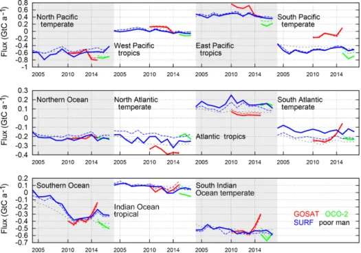
Figure 9 reformulates the bias statistics of Fig. 8 on a map of the differences between the absolute biases of the OCO-2 and SURF inversions. As for the programme biases, some points are more robust than others (due to varying amount of data), but there is some large-scale coherence, with better performance of SURF in the Southern Hemisphere (as could already be seen in Figs. 7 and 8) and in the central and eastern US, whereas OCO-2 yields smaller biases in the Northern Hemisphere subtropics and Europe. Other parts of the globe are less consistent such as the western Pacific edge or boreal America.

3.4 Pixel attribution

Liu and Bowman (2016) proposed a method to quantify the impact of flux changes over the globe on the corresponding change in the mean squared error (MSE) of the transport model simulation with respect to n independent measure-ments. They demonstrated it in the case of the flux changes from their prior values to their posterior values within the approximations of a linear transport model M (including the sampling operator at the measurement time and location) and of an unchanged initial state of CO2. It is actually valid for

other types of changes within an inversion, provided they re-spect the tangent linear hypothesis for the transport model. The change in the MSE (δMSE) is expressed as a finite sum of terms. There is one term for each element i of the inversion control vector (i.e. a CO2flux at a given time and location,

or some part of the 3-D initial state of CO2):

δMSE = 6iδfi[MT(δc1+δc2)]i. (1)

Term i is the product of the corresponding change in the con-trol vector (i.e. a scalar δfi), times the corresponding row

of the transpose of the linear model M, times (dot product here) the vector of the sum of the differences between the two model simulations (one, c1, before the change in the control

vector and one, c2, after the change) and all verification

mea-surements (δc1+δc2, both vectors with dimension n).

Inter-estingly, the second product in this formula can be calculated by the adjoint code of the transport model, if it exists, which is the case for LMDz (Sect. 2.2). Further detail is given in Liu and Bowman (2016).

We apply this approach to interpret the difference be-tween the OCO-2-based and the surface-based inversions us-ing LMDz5A. The overall MSE is very similar between both (1.52ppm2), but the relative performance still varies in space and time (Figs. 8, 9) and we hope to extract some further in-sight into the relative merits of each dataset. In practice, we

(13)

Figure 6. Grid-point budget of the natural CO2fluxes for the year 2015. In the sign convention, positive fluxes correspond to a net carbon

source into the atmosphere.

compute δc1+δc2using the LMDz model linearised around

the inversion prior simulation in order to respect the underly-ing hypothesis. However, some inconsistencies for the initial state of CO2could not be completely removed between δc1

and δc2due to the different starting date of each inversion.

The map of the sum of all contributions of the flux changes δfi (from the surface-based inversion to the OCO-2-based

inversion) at a given pixel to the change in MSE (δMSE) is presented in Fig. 10. Positive values occur when the OCO-2-based fluxes increase the MSE relative to the surface-OCO-2-based fluxes. This happens in the western contiguous US, north-eastern South America, western Europe, Turkey, the West Siberian Plain and eastern Siberia. Contributions to reduce the MSE (negative values) are mostly in Alaska and the east-ern contiguous US, westeast-ern South America, southeast-ern Africa, South and Southeast Asia, and Indonesia. No noticeable con-tribution is seen over the ocean, where OCO-2 retrievals have not been assimilated. By construction, regions that are not well observed downstream by aircraft have lesser contribu-tions, like in Africa. This feature makes the relative magni-tude of the patterns among each other not very informative regarding the flux quality. Therefore, we will pay more at-tention to the sign of the dominant patterns.

The map in Fig. 9, which refers to differences in absolute biases within moving windows, is, in principle, not directly comparable with Fig. 10, which refers to MSEs. However, bias changes are much larger than standard deviation changes (Fig. 8) which makes the map of root-mean-square errors

(RMSEs, not shown) very similar to Fig. 9. Differences be-tween the patterns in Fig. 9 in the space of free-tropospheric mole fractions and those in Fig. 10 in the space of fluxes are linked to the way CO2is transported between the surface and

the free troposphere. Dominating westerlies outside the trop-ics bring the positive flux contributions in Fig. 10 to the west of the positive RMSE variations in Fig. 9, like from the west-ern to the eastwest-ern US, or, at a much larger scale, from Eura-sia to Alaska. Similarly, negative flux contributions from the eastern US induce negative RMSE variations in the central North Atlantic Ocean, and tropical easterlies link the neg-ative flux contributions from southern Africa to the negneg-ative RMSE variations in the tropical Atlantic Ocean. The distance between the flux signal and the free-tropospheric signal im-plies an important role for the transport model in attributing the latter to the former; therefore, these patterns should be considered with caution, as is the case for inversion systems in general.

4 Discussion

Interest in atmospheric CO2observations has grown

dramati-cally over the last decade, with the hope that they can reliably quantify the evolution of the CO2 sources and sinks.

How-ever, a suite of physical and statistical models is needed to estimate the latter from the former. For instance, the link be-tween some of these observations, like the satellite retrievals, and measurement standards is not direct and needs to be

(14)

em-Figure 7. Model-minus-observation absolute differences and stan-dard deviations over the GOSAT period per measurement pro-gramme for the surface-based inversion (SURF, red line), the GOSAT-based inversion (GOSAT, blue line) and the poor man’s inversion (shaded area). Inversions with LMDz5A (LMDz6A) are shown using continuous (dashed) coloured lines. The number of measurements per site, campaign or programme varies between 113 (BNE) and 901 846 (CON). The programme definitions are given in Table 1. They are ranked by increasing mean latitude (north is on the right), irrespective of their latitudinal coverage (which is large at several tens of degrees for ORC, TOM, HIP and CON). These mean latitudes are shown in the middle of the panel. For each pro-gramme, a green circle appears in the upper panel if the difference between the GOSAT bias and the SURF bias using LMDz5A is sta-tistically significant (see the main text for a definition) and exceeds 0.15 ppm. Similarly, a red (blue) circle indicates that the difference between LMDz5A and LMDz6A for SURF (GOSAT) is statistically significant and exceeds 0.15 ppm.

pirically made. We also lack measurements dedicated to the development and validation of atmospheric transport mod-els, in particular for sub-grid-scale processes. Therefore, the various underlying models are still in development and our current source–sink estimation capability is not clear: there is no consensus about the latitudinal distribution of the natu-ral carbon fluxes (Le Quéré et al., 2018) or about the carbon

Figure 8. Same as Fig. 7 for the OCO-2 period. The number of measurements per programme varies here between 133 (CRV) and 211 358 (CON).

budget of relatively well-documented regions like Europe (Reuter et al., 2017). Here, we have defined quality measures for global inversion systems in order to evaluate the current skill of global inversions, via the example of the CAMS in-version system. By focussing on a specific inin-version system, we have avoided the problem of heterogeneity of TransCom-type ensembles, which gather systems with various degrees of sophistication (resolution of the transport model, size of the control vector), but we still varied the assimilated data (surface or satellite) and the transport model in order to gen-erate a small inversion ensemble.

In practice, quality measures for a data assimilation sys-tem must rely on unbiased and independent data (Talagrand, 2014). The property of being unbiased means that the errors are null on statistical average. The property of independence means that the errors affecting the verification data must not be correlated with the errors affecting the observations that have been used in the inversion. Ideally, the verification data should be the carbon fluxes to be evaluated, but in the spe-cific case of global inverse systems, the spatial resolution of existing flux observations (of the order of a hundred metres)

(15)

Figure 9. Difference between the model-minus-observation abso-lute differences in 10◦ moving windows (a). Negative (positive) values denote areas where the OCO-2-based inversion has smaller (larger) biases than the surface-based inversion. Both inversions use LMDz5A. Panel (b) gives the number of data that contribute to the bias computation in each 10◦moving window. Biases are only com-puted in the windows where there are more than 100 measurements.

Figure 10. Contribution of the grid-point flux changes to the change in the variance of CO2 model–measurement differences between

the OCO-2-based inversion and the surface-based inversion (vari-ance of the former minus vari(vari-ance of the latter), in parts per million squared. Both inversions use LMDz5A. Note that the fluxes them-selves are illustrated in Fig. 6a and c.

is much smaller than the spatial resolution of global transport models (larger than a degree). Therefore, one has no option but to evaluate the analysed CO2fields (that are the

combi-nation of the analysed surface fluxes, of an analysed initial state of CO2 and of the transport model used in the

inver-sion) rather than the analysed surface fluxes alone, both of which are related through mass-conserving transport in the

global atmosphere. This can be done with atmospheric ob-servations like those listed in Sect. 1: surface measurements, aircraft measurements, TCCON retrievals, AirCore measure-ments or satellite retrievals. We remove TCCON and the satellite data from the list on the criterion that they are biased (Fig. 9 suggests that we are interested here in signals that are smaller than the TCCON trueness; see also the discus-sion in Chevallier, 2018b), the surface data on the criterion of independence (the surface data in ObsPack-type databases that are well simulated by the transport models are usually assimilated), and the AirCore data because of limited time and space coverage so far. This leaves aircraft data, how-ever scarce they are, as an obvious choice to define objective measures of the quality of the inversion systems, when they are not assimilated. They have served this role in the past to some extent, starting from Peylin et al. (2007) or Stephens et al. (2007) (see also Pickett-Heaps et al., 2011; Basu et al., 2014; Houweling et al., 2015; Frankenberg et al., 2016; Le Quéré et al., 2018; Crowell et al., 2019), but few aircraft mea-surement programmes have been used so far and, as a conse-quence, their use has rarely been formulated in terms of qual-ity assurance or qualqual-ity control processes for atmospheric in-versions. Compared with previous studies, we benefit from a much larger number of aircraft measurements over the globe in the free troposphere (600 000 for the OCO-2 period and twice as many for the GOSAT period) and from more recent satellite retrievals.

We have only used data between 2 and 7 km a.s.l., where the age of air varies significantly (Krol et al., 2018). Aircraft data in this region of the atmosphere only sample a portion of the carbon cycle. With their sparse coverage in places, they may miss some of the tropical flux signal that can reach higher levels within a few days, but flux errors compensate for this at the global scale such that errors in the tropics that would not be directly seen will likely induce errors elsewhere that can be seen. Conversely, our 5 km wide layer still repre-sents a large portion of the column observed by the satel-lites. However, with the use of individual pointwise mea-surements (rather than profile averages), we hope to have minimised the possible advantage given to the satellite inver-sions with respect to the surface-based inverinver-sions. The gra-dient between mole fractions in the boundary layer and the free troposphere is also informative (Stephens et al., 2007). It provides complementary information about inversion quality, provided that the minority of measurements above urban ar-eas or in the vicinity of assimilated surface sites are excluded. This has not been explored here. Most of the aircraft mea-surement programmes here are over North America, but the majority of measurements are provided by the CONTRAIL programme, as noted in the legends of Figs. 7 and 8. CON-TRAIL samples air at our study altitudes above many cities outside North America; it also represents 74 % of all data for the GOSAT period and 39 % for the OCO-2 period.

For our ensemble of six Bayesian inversion results, we have seen that large differences in the estimated annual

(16)

sub-continental fluxes (GOSAT-based vs. surface-based results) are paralleled by a different quality of fit to the aircraft data, with GOSAT-based results not performing as well. An addi-tional poor man’s inversion, which simply adjusts very recent bottom-up flux estimates with the annual global growth rate, has larger differences than the surface-based and the OCO-2-based inversions in terms of flux and the aircraft data. Chang-ing the transport model only affected the flux estimation at the scale of TransCom-type regions: no benefit could be seen with respect to aircraft data, despite 6 years of model devel-opment within the CMIP framework by the LMDz team and despite improved nudging meteorological variables between the two versions (from ERA-Interim to ERA5). This result is consistent with our study of the parent model of our offline model in forward mode (Remaud et al., 2018) and suggests that LMDz transport errors play a much smaller role in the quality of our inversion results than the choice of assimilated data. This may be different for previous versions of LMDz: for instance, the refinement of the vertical grid in our version of LMDz from 19 to 39 layers had a major impact (Cheval-lier et al., 2014). This may be different for some other offline models: for example, Schuh et al. (2019) highlighted regrid-ding problems within one model to explain some large dif-ferences with another one. In comparison to the GOSAT re-sults, or to previous OCO-2 inversion results (Crowell et al., 2019), OCO-2-based annual fluxes are surprisingly close to the surface-based fluxes (usually within 1σ of the Bayesian uncertainty of the surface-based fluxes). Consequently, the aircraft data used here do not allow us to distinguish be-tween the quality of OCO-2-based fluxes and surface-based fluxes. The poor man’s inversion still performs worse despite the contribution of a recent dynamic global vegetation model simulation (i.e. simulation ORCHIDEE-trunk in Le Quéré et al., 2018), showing that the OCO-2 performance is not triv-ial. From our results, we cannot draw general conclusions about OCO-2 retrievals nor about GOSAT retrievals, because our study is limited to two specific retrieval datasets. Takagi et al. (2014) showed large differences between different re-trieval algorithms for GOSAT, and it is still possible that we would get similar results between OCO-2 and GOSAT if we used the same retrieval algorithm.

Following Liu and Bowman (2016), we attribute the sim-ulation error changes in the free troposphere for the OCO-2 period to flux differences in specific regions of the globe. We find a rather homogeneous geographical distribution of the flux performance with OCO-2-based fluxes and surface-based fluxes alternating as those with the best performance over continental land masses. This adjoint analysis also il-lustrates the large footprint of our aircraft data in the free troposphere in terms of flux information, which prevents us using them for the evaluation of local fluxes, given our choice of altitude range between 2 and 7 km a.s.l.

5 Conclusions

Within the limitations imposed by the use of two differ-ent verification periods, the tested bias-corrected OCO-2 re-trievals perform better than the tested GOSAT rere-trievals in our inversion system. Upstream, both inferred flux time se-ries do not overlap with each other at all scales studied here (for instance in the tropical lands) in terms of both the mean and variability. This prevents us from computing flux anoma-lies from one vs. the other. Within the study time frame, it was not possible to test more than a couple of different ver-sions of the GOSAT retrievals (despite large differences be-tween GOSAT retrieval algorithms, Takagi et al., 2014) or other ways to assimilate the OCO-2 retrievals. Indeed, each one of our six Bayesian inversions represented a large com-putational effort that lasted between 4 and 6 weeks on a par-allel cluster. Therefore, we could not identify the distinctive asset of OCO-2 vs. GOSAT in our system: either the data density, the data precision, the data trueness (linked both to the quality of the physical retrieval scheme and to its em-pirical bias-correction) or a combination of these qualities at once. Further, other GOSAT-based inversions could be more competitive if made differently (e.g. with a different bias-correction), while other OCO-2-based inversions (e.g. with a different transport model or with different retrievals), or our inversion with ACOS v9 retrievals after our study period (e.g. if the empirical bias-correction is less efficient for later months), could still be found deficient for carbon specialists. As we have shown, aircraft data can help with ranking the skill of these alternative inversion configurations among one another and vs. ours (all data used here, apart from the recent INPE data, are publicly available).

This validation strategy assumes that airborne measure-ment programmes are continued while new satellite obser-vations are made, and that these programmes fairly sample the diversity of CO2plumes in the free troposphere. In this

respect, the situation is not satisfactory at present in some parts of the world, such as Africa. We also need better cov-erage to accompany the better quality of inversion results expected in the coming years. This validation strategy also implies that aircraft data remain independent of the inversion system, and, therefore, that observations dedicated to the free troposphere (aircraft or satellite partial column retrievals) are not assimilated. This is usually the case, for instance because of the challenging characterisation of model errors in simu-lating aircraft profiles or because systematic errors for partial column retrievals are too large. Zhang et al. (2014) and Alden et al. (2016) presented a different strategy in which aircraft profile measurements are assimilated: a compromise has to be found between exploiting valuable data directly (in par-ticular in areas void of surface measurements), or keeping them for validation.

Finally, the evidence provided by aircraft measurements in the free troposphere suggests that the quality of some OCO-2 retrievals over land is now high enough to provide results that

(17)

are comparable in credibility to the reference (but sparse) sur-face air sample network, within the above-mentioned limits. For ocean retrievals, this remains unclear as OCO-2 ocean soundings were not tested in this work. The consistency of re-sults from the surface- and OCO-2-driven inversions, in stark contrast to the bottom-up fluxes or to the GOSAT-driven in-version, does not seem to be fortuitous. It may reinforce some specific conclusions from the surface network, for instance pertaining to the location of the land sink in latitude during the recent years. Remaining differences between fluxes from these two flux inversion types require further analysis and un-derline their complementarity. The best results may now be obtained by inversions that simultaneously assimilate both observation types.

Data availability. The aircraft measurements are available from https://www.esrl.noaa.gov/gmd/ccgg/obspack/ (last access: 21 November 2019). The OCO-2 data can be obtained from http://co2.jpl.nasa.gov (last access: 21 November 2019) and were produced by the OCO-2 project at the Jet Propulsion Laboratory, California Institute of Technology. The CAMS v18r1 product can be obtained from http://atmosphere.copernicus.eu/ (last access: 21 November 2019), and the GOSAT retrievals are available from http://climate.copernicus.eu/ (last access: 21 November 2019). All inversion results can be obtained upon request to [email protected].

Author contributions. FC designed the experiments and carried them out. FC, MR, CWO’D, DB and PP analysed the results. MR and AC adapted the LMDz6A model for tracer transport. FC and MR prepared the paper with contributions from all co-authors.

Competing interests. The authors declare that they have no conflict of interest.

Acknowledgements. The authors are very grateful to the many people involved in the surface, aircraft and satellite CO₂ ob-servations and in the archiving of these data that were kindly made available for this study, including Hartmut Bösch and Jas-deep Anand at the University of Leicester, the ObsPack team and LaGEE, and the Greenhouse Gases Laboratory from INPE. The Carbon in Arctic Reservoirs Vulnerability Experiment (CARVE) is an Earth Ventures (EV-1) investigation, under contract with the National Aeronautics and Space Administration. The Atmo-spheric Carbon and Transport (ACT) – America project is a NASA Earth Venture Suborbital 2 project funded by NASA’s Earth Sci-ence Division (grant no. NNX15AG76G to Penn State). This work was performed using HPC resources from GENCI-TGCC (grant no. 2018-A0050102201). The authors thank Hartmut Bösch, François-Marie Bréon, Grégoire Broquet, John B. Miller, Brit-ton B. Stephens, Jeff Peischl, Sander Houweling, the editor and the three anonymous reviewers for constructive discussions about these results and how they are presented. Bianca Baier, Kenneth J. Davis,

Luciana Gatti, Kathryn McKain and Charles E. Miller provided use-ful details regarding some of the measurement programmes.

Financial support. This research has been supported by the Coper-nicus Atmosphere Monitoring Service, implemented by the Euro-pean Centre for Medium-Range Weather Forecasts on behalf of the European Commission (grant no. CAMS73), and from ESA through contract no. 4000123002/18/I-NB RECCAP-2.

Review statement. This paper was edited by Federico Fierli and re-viewed by three anonymous referees.

References

Alden, C. B., Miller, J. B., Gatti, L. V., Gloor, M. M., Guan, K., Michalak, A. M., Laan-Luijkx, I. T., Touma, D., An-drews, A., Basso, L. S., Correia, C. S., Domingues, L. G., Joiner, J., Krol, M. C., Lyapustin, A. I., Peters, W., Shiga, Y. P., Thoning, K., Velde, I. R., Leeuwen, T. T., Yadav, V., and Diffenbaugh, N. S.: Regional atmospheric CO2

in-version reveals seasonal and geographic differences in Ama-zon net biome exchange, Glob. Change Biol., 22, 3427–3443, https://doi.org/10.1111/gcb.13305, 2016.

Basu, S., Krol, M., Butz, A., Clerbaux, C., Sawa, Y., Machida, T., Matsueda, H., Frankenberg, C., Hasekamp, O. P., and Aben, I.: The seasonal variation of the CO2flux over Tropical Asia

es-timated from GOSAT, CONTRAIL, and IASI, Geophys. Res. Lett., 41, 1809–1815, https://doi.org/10.1002/2013GL059105, 2014.

Bocquet, M., Wu, L., and Chevallier, F.: Bayesian design of con-trol space for optimal assimilation of observations. I: Consistent multiscale formalism, Q. J. Roy. Meteor. Soc., 137, 1340–1356, https://doi.org/10.1002/qj.837, 2011.

Bolin, B. and Keeling, C. D.: Large-scale atmospheric mix-ing as deduced from the seasonal and meridional varia-tions of carbon dioxide, J. Geophys. Res., 68, 3899–3920, https://doi.org/10.1029/JZ068i013p03899, 1963.

Bösch, H. and Anand, J.: Product User Guide and Specifica-tion (PUGS) – ANNEX A for products CO2_GOS_OCFP, CH4_GOS_OCFP & CH4_GOS_OCPR. C3S re-port ref. C3S_D312a_Lot6.3.1.5-v1_PUGS_ANNEX-A_v1.3, available at: http://datastore.copernicus-climate. eu/c3s/published-forms/c3sprod/satellite-carbon-dioxide/ product-user-guide-annex-a-v1.3.pdf (last access: 21 Novem-ber 2019), 2017.

CarbonTracker Team: Compilation of near real time atmospheric carbon dioxide data; obspack_co2_1_NRT_v4.3_2018-10-17; NOAA Earth System Research Laboratory, Global Monitoring Division, https://doi.org/10.25925/20181017, 2018.

CEOS Atmospheric Composition Virtual Constellation Green-house Gas Team: A constellation architecture for monitoring carbon dioxide and methane from space, Report from the Com-mittee on Earth Observation Satellites (CEOS) Atmospheric Composition Virtual Constellation (AC-VC), available at: http://ceos.org/document_management/Virtual_Constellations/