HAL Id: halshs-01179057
https://halshs.archives-ouvertes.fr/halshs-01179057
Submitted on 21 Jul 2015HAL is a multi-disciplinary open access archive for the deposit and dissemination of sci-entific research documents, whether they are pub-lished or not. The documents may come from teaching and research institutions in France or abroad, or from public or private research centers.
L’archive ouverte pluridisciplinaire HAL, est destinée au dépôt et à la diffusion de documents scientifiques de niveau recherche, publiés ou non, émanant des établissements d’enseignement et de recherche français ou étrangers, des laboratoires publics ou privés.
Shapley Allocation - the effect of Services on
Diversification
Peter Mitic, Bertrand K. Hassani
To cite this version:
Peter Mitic, Bertrand K. Hassani. Shapley Allocation - the effect of Services on Diversification. 2015. �halshs-01179057�
Documents de Travail du
Centre d’Economie de la Sorbonne
Shapley Allocation — the effect of Services
on Diversification
Peter M
ITIC,Bertrand K. H
ASSANIShapley Allocation – the effect of Services on Diversification
1Peter Mitic
Santander UK
2 Triton Square, Regent’s Place, London NW1 3AN Email: [email protected]
Tel: +44 (0)207 756 5256
Bertrand K. Hassani
Universitė Paris 1 Panthėon-Sorbonne, CES UMR 8174 106 bouvelard de l'Hôpital, Paris Cedex 13, France and
Santander UK
2 Triton Square, Regent’s Place, London NW1 3AN Email: [email protected]
Tel: +44 (0)207 756
Abstract
The Shapley method is applied to capital allocation in the context of a simple business model, where many business units supported by services. In this model the services are capable of either reducing the capital payable by the business units, or the opposite. A simple model of evaluating the value of coalitions is proposed, with a modification if a service is a member of the coalition. A closed form formula for the Shapley allocation to all players is derived, thus eliminating combinatorial problems.
Keywords Allocation ∙ Shapley ∙ Operational Risk ∙ Diversification ∙ Service ∙ Game Theory ∙ Capital Value
JEL Classification C71
1 Introduction
A business model in which a large organisation is partitioned into smaller interacting units has been well established for many years. Generalising somewhat, some of these sub-units may be actively engaging in producing products of the business. In this paper we will refer to these as ‘Business Units’ (BU for short). Others aid them in this process. For example, they may provide and maintain IT systems, do catering, provide waste management facilities or carry out a supervisory function. We will refer to these as ‘Services’. The way in which Services interact with Business Units may be complex, but the basis of this service model is that ‘Business Units’ use services provided by ‘Services’. See, for example, Levitt (1972) for a detailed discussion of a basic version of this model. More recently the model has been modified to take into account new innovations in technology, and the idea of a ‘solution provider’ (SP for short) has emerged. A summary of an enhanced ‘service’ business model is discussed in Cambridge (2011). The type of service offered may be very specialist, and may thereby become part of the operational structure of the organisation that uses the service. For example, the service may be to provide a cloud computing infrastructure, or to manufacture an essential component. In this way the SP becomes a component of production in its own right.
The term ‘business model’ has been, and continues to be, used in many contexts. Magratta (2002) and Shafer et al (2005) provide some discussion of a more general context for the term ‘business model’. Broadly they cover the general area of ‘strategies for running a business’. The service model outlined above is clearly one of these, but we will limit the discussion in this paper to a particular issue: that of allocation of a particular resource among BUs who have a relationship with SPs. For reference, a wider discussion of ‘business model’ might cover items from the following list. This list is not exhaustive.
Add-on model: there is a core product plus extras that can be bought
Franchise model: an organisation buys the right to trade under a particular name
Advertising model: an organisation derives its revenue from advertisers
Subscription model: the consumer pays for a resource no matter how much of that resource they use
Pay-as-you-go model: the consumer only pays for what is used.
These and many any other are discussed by Lai et al (2006). As discussed below, the Pay-as-you-go model is an essential part of the Shapley allocation process, which we will apply to the allocation problem which is the subject of this paper.
2 Diversification and Allocation in Operational Risk
In this section we introduce the relevant elements of this analysis: service types, the value of a BU, diversification, and allocation.
2.1 Service Types
In this paper we distinguish between two types of service. In the first, a BU buys a service from a SP, thereby adding to the total cost of production. There is a real flow of cash from the BU to the SP. For example, the BU buys IT services, or pre-fabricated parts, etc. Overall, the service may be bought because it is more cost effective to do so than to provide the service ‘in house’. Alternatively, there may be an accounting justification for buying a service. In the second type of service, the SP provides a service which reduces a cost to the BU. There may be no actual cash flow, but there is an implied cash flow from the SP to the BU. An example is arisk department. Its job is to reduce and manage the risks taken by other business units so that the aggregated amount of losses is lower than if the risk department was not present. Up to a certain extent, the income of the risk department is equal to the theoretical amount the risk department enables it to save.
We will analyse a basic service model in terms of a particular context. Each BU must pay an amount of cash hereinafter termed ‘capital’. The total amount to be paid is known, but the amount to be paid by each BU has to be determined. In other words, there must be an allocation of capital to the BUs. Each BU is a risk taker, and interacts with the two types of service. Each BU buys services that allow it to function (e.g. IT support). Effectively the amount of capital payable by each BU is increased by having to pay for the service. Each BU also benefits from the services of a risk department that allows them to function better (i.e. with reduced risk). The risk management service reduces the amount of capital payable by each BU. The overall effect is a balance in the flow of capital to and from each BU.
2.1.1 Definitions: receiver and emitter Service Provider
A service (such as Risk Management) which reduces capital payable by a BU will be termed a ‘receiver’ of capital. Such a SP effectively receives capital from the BU, and transmits it for use in another part of the organisation. A service (such as IT) which increases capital payable by a BU will be termed an ‘emitter’ of capital. If the initial capital of an emitter SP is zero (because its ‘riskiness’ is zero), it will end up with a negative capital after transfer to BUs. In terms of game theory, the game defined by the BUs and SPs in an organisation, with rules that determine how capital should be transferred, is zero-sum.
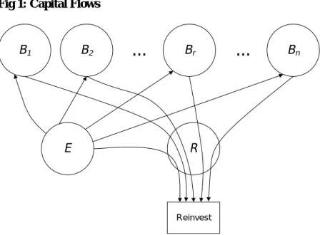
There is generally an interaction between a receiver SP such as Risk Management, and an emitter SP such as IT. The receiver sees the emitter SP as another business unit, and the emitter sees the receiver similarly. In the specific case of Risk Management and IT, Risk Management receives capital from IT, thereby reducing the capital of IT. Figure 1 shows a generalised case of capital flow, with a group of n BUs, B1, B2, …, Bn, one emitter SP (E) and one receiver SP (R). The receiver does not retain capital: it routes capital to a ‘reinvestment’ pot.
Fig 1: Capital Flows
B1 B2
...
Br...
BnE R
Reinvest
There can also be a contagion effect associated with a problem due business disruption of a SP such as IT. An example is the RBS/NatWest cash machine failure in December 2013. See IBTimes (2013) for example. Customers were unable to use cash machines, do online banking, and direct debits were not collected. The cost to a BU is therefore not just a fee payable: it has to absorb costs of a failure, which may be considerable.
2.2 Riskiness and Value
Given that the BUs in this analysis are risk-takers, the extent to which they take risks is important. We use the term ‘riskiness’ in a very loose sense to indicate a degree of risk that a BU undertakes. ‘Riskiness’ may be measured precisely. The list below shows several ways in which ‘riskiness’ could be measured, with respect to a given historic time period.
Measure the mean or maximum loss incurred by the BU
Calculate value-at-risk (VaR) or expected shortfall (ES) of simulated losses
Informed scoring by domain experts
We will use the term ‘riskiness’ to mean an assessment of risk incurred, and measured by any of the above methods, or any other appropriate method. We also use the term ‘value’, which is more common in game theory, to be synonymous with ‘riskiness’.
In our case, we are trying to allocate capital obtained from a risk based methodology. Therefore, the riskiest BU, who generates the largest loss amount, would require more capital to cover their risks. Unfortunately this strategy is neither risk management sensitive or fair: it does not reward the BU who is trying to manage its risk in the best way possible.
It is assumed in this paper that no BU is ‘dominant’ over any others. We use the term loosely here to indicate that a particular BU may be able to influence its capital allocation more than others. The issue of dominance required separate analysis, and there is no definitive formal definitions of ‘dominance’. A discussion in a very different context (aircraft landing fees) may be found in Littlechild and Owen (1973), and Littlechild and Thompson (1977).
2.3 Diversification
When operational risk is measured in terms of a calculated capital value, if the losses for all BUs are aggregated, the capital value of the aggregation is expected to be less than the sum of capital values of all the BUs. The discrepancy is a measure of ‘diversification’. More directly, diversification can be measured as a multiplicative factor of the sum of capital values of all the BUs. In some cases the operational risk diversification can appear to be huge due to an averaging effect of combining losses. A fuller account of the diversification effects on capital value is given by Monti et al (Monti 2010). They link diversification to the dependency structure between operational risk UoMs, estimated via correlations.
2.4 Pro Rata Allocation
'Pro Rata' allocation is an intuitive allocation method, which appears to be 'fair'. Allocation is in proportion to some measureable metric: very often 'usage'. 'Pro Rata' allocation does not account for the benefits of cooperation: it rests solely on the measured metric.
Given a group of n business units B1, B2,…,Bn, with respective values (i.e. riskiness) v1, v2,…,vn, the Pro Rata allocation to business unit r, PR(r), is given by (1), with V = v1 + v2 + … + vn, (which is the total amount to be allocated):
r r r V v V v B PR (1) 2.5 Shapley AllocationIn this analysis we apply the Shapley allocation method to allocate capital to a large number of BUs, and introduce SPs as a necessary part of the allocation. Shapley’s achievement was to propose, a set of rules to define ‘fairness’ in allocation, an allocation formula supported by an associated algorithm for applying it, and a proof that shows that the algorithm derives the optimal (i.e. the ‘fairest’) allocation. The original paper is in (Shapley 1953). His method has been used extensively ever since, and he received the 2012 Nobel Prize for Economics in recognition for its importance.
Shapley's original allocation formula gives the allocation for a member i, in a coalition C, as
𝜑𝑖 = ∑ (𝑠 − 1)! (𝑛 − 𝑠)! 𝑛! [𝑣(𝑠) − 𝑣(𝑠\{𝑖})] 𝑖∈𝐶 . (2) where v(•) is the 'value' (i.e. riskiness) of the coalition, s, and n is the number of members in C. The notation has been changed slightly from the original. The important points to note here are that each coalition s has a 'value', and the term [v(s) - v(s-i)], which represents marginal value added when member i joins coalition s. This term is an important feature of the analysis of this paper. The sum term, with division by n! indicates a calculation of a mean value, and the term (𝑠 − 1)! (𝑛 − 𝑠) indicates that all permutations of s need to be considered.
Shapley allocation is, in principle, a 'fair' allocation method because it accounts for the benefits of forming coalitions. This could be translated into working efficiently in a professional environment.
The justification "Shapley allocation is the fairest means of allocation because business units are charged only for losses they incur" is the reasoning most likely to be seen as credible.
2.5.1 Problems in applying the Shapley Allocation
Shapley's allocation formula, equation (2), implies an algorithm for calculating Shapley values which gives an insight into the method that equation (2) does not. The algorithm proceeds by considering all permutations of players. For each permutation, the marginal effect of a new player to an existing coalition is considered. The Shapley value is then the mean value of the marginal contributions for each player.
Applying this algorithm illustrates three points. First, if all participants cooperate, it is possible to reduce the amount allocated to each of them relative to the 'Pro Rata' method. Second, although values of intermediate coalitions are needed, in practice they do not exist explicitly. They have to be estimated by an appropriate method. Third, the combinatorial complexity of using the algorithm for a large number of participants is immense. In practice, ‘large’ means six or more. Typically we would deal with 8 to 20 BUs, and in some cases many more. We therefore have to develop an allocation method that can cope with the combinatorial problems associated with a large number of BUs in the Shapley process.
If it is not feasible to examine all permutations of all members of a coalition, the possibility of sampling exists, but only in conjunction with a way to find the value of all coalitions in the sample. Liben-Nowell et al (Liben-Nowell 2012), and Castro et al (Castro 2009) give an account of some sampling strategies, with an indication of sample size required. We have found that approximately 250000 samples are needed to give allocations close to the exact outcomes for a total of five BUs.
Consequently, we propose an alternative approach, which implements the Shapley algorithm implied by equation (2), but avoids the associated pitfalls.
2.6 Allocation to a service: a general context
The Shapley method has been applied to the problem of allocating service costs in many situations. We mention a small selection.
Linhart et al (1995) allocate the fixed cost of caller IDs (which is the service) in the context of companies in a telecommunications system. They use two methods: Shapley and 'Incremental Recording'. For the latter method they allocate points to each company involved in a call, and then allocate using the Pro Rata method, based on accumulated points. They model the service cost by a linear function of the number of identifiable incoming calls. We will use a similar idea for modelling added value when there are a large number of participants.
Butler and Williams (2006) share fixed cost in a general context of 'facilities' and 'customers', using an Integer Programming technique. They formalise a concept of 'fair' allocation: savings are equalised over all possible consortia, thereby providing a parallel with the Shapley method.
Junqueira et al (2007) use the Aumann-Shapley method (Aumann and Shapley 1974) to allocate service costs in the context of networked users in an energy market. 'Fair' allocation implies that the charge for
a service is proportional to the degree of use of that service, and to efficient location of the service. They consider a network with about 10000 nodes, and simulate the marginal cost of transmission by a linearized power flow model. In many ways this method has a parallel with the methods proposed in this paper, in that a small number of parameters apply for all nodes.
Dehez (2011) provides comprehensive accounts of fixed cost allocation and the theory behind the Shapley method, and also gives a simple numerical example
3 Shapley Allocation of Capital charges
In this section we apply allocation of capital charges using the Shapley algorithm. The starting point is a game played between n Business Units B1, B2,…,Bn, with a service S, making n+1 players in all. The service can be one of two types: emitter or receiver. The allocation game is zero-sum, so if there are winners, there must also be losers. Looking at this another way, any initial capital value is redistributed in the allocation process, with no inflow or outflow of capital. Each player is associated with a ‘value/riskiness’. A ‘risky’ business unit has a high value, and a less ‘risky’ business unit has a low value. It is possible for a BUs value to be negative. The interpretation is that the BU must be paid a capital charge, rather than having to pay the charge.
In this paper we use terms from game theory, since allocation is often studied as part of game theory. In particular, the terms ‘Business Unit’ and ‘BU’ will be used synonymously with the term 'player' from game theory. The term 'coalition' means a collection of players who cooperate.
3.1 Shapley formulation
In some contexts, for example operational risk, capital values of coalitions are not immediately available. Even if they were, if there are many players there is a considerable combinatorial problem in finding a solution by the Shapley method. Furthermore, the final results must be seen as 'fair' in a 'business as usual' sense. We therefore make assumptions.to make the problem tractable, and to emphasise the effect of the service.
The value of a coalition comprising a subset of the “B” business units is the sum of values of the business units in the subset. This implies that any coalition of “B” business units is not diversified.
The service S has zero initial value.
If S is a member of a coalition with subset of the “B” business units, the value of the coalition is the sum of values of the “B” business units, multiplied by a constant factor. S allows a diversification for the other members of the coalition
All “B” business units are equivalent in the way they are analysed. Only the service is different.
3.2 Notation
The 'value', v(B), of a single player B is a measure of the risk associated with B (i.e. its ‘riskiness’). For example, in operational risk this might be a suitable quantile on a fitted loss distribution. The number of players in a coalition C is denoted by |C|.
Let J be an indexing set for a subset of the integers 1..n. Then ⋃𝑗𝜖𝐽(𝐵𝑗) denotes a coalition of |J|
members.
The value of an individual player Br (i.e. a player not in a coalition) will be denoted by vr. More generally, the value of any coalition C will be denoted by v(C).
The marginal allocation to a player Bwill be denoted by M(B), with a subscript when appropriate. This is the difference in values of an existing coalition before and after Bjoins.
A cost function defines how the addition of a new player P to a coalition C affects the value of that coalition. In this paper, cost functions will be defined explicitly.
The Shapley value of player Br is denoted by SH(n, r). At a later stage we will compare the Shapley allocation to Br with the corresponding allocation derived from the Pro Rata method, which will be defined when the comparison is made. The Pro Rata value of player Br is denoted by PR(n, r).
3.3 Numerical examples
In advance of deriving results in a general case of n players, we will consider two short numerical cases to illustrate the role of two distinct types of service. In the first case, the service transfers capital from the “B” business units to the service. In the second case, the service transfers capital to the “B” business units from the service. Both types of service should carry risk capital in their own right, but does not. The global diversification benefit is obtained from the largest coalition possible (the 'grand' coalition). Following the numerical examples, we demonstrate that there is a closed-form expression for the Shapley allocation for any of the players in the domain, given the distinction between service and business unit.
3.3.1 Shapley analyses by enumeration of cases
In this paper we do not intend to give a detailed explanation of the process for calculating a Shapley value. The literature does not abound with such explanations, and those that exist tend to be short of detail. Garcia-Diaz and Lee (2013) provide a simple example, but it is not set out in a useful form. Dehez (2011) gives another example, with a good exposition of the supporting theory of the Shapley method. Tarashev et al (Tarashev 2009) show a similar calculation using operational risk capital values. They use a tabular form, but do not clarify the point that it is useful to group all marginals for a player in the same column.
The essential principle embodied in Equation (1) is to enumerate all permutations of players, and for each permutation, the marginal contribution to each coalition when a new member enters. As an example, suppose that there are five “B” players B1, B2, B3, B4, and B5, with a service S. Consider one of the 6! coalitions: {B2, B3, S, B1, B4, B5}. B2 enters first, and its marginal value is v(B2), which should be attributed to B2 (i.e. placed “in the B2 column”). Then B3 enters, and the marginal value attributed to B3 is v(B3, B2) - v(B2). All other members of the coalition are processed in the same way. When all such coalitions have been considered, the Shapley value of each player is calculated as the mean value of the marginals for each player.
The process described above is easy to apply for a small number of players (<6), but when more are involved, it is useful to adopt an alternative technique. This is to consider each player at a time, and calculate the marginals for that player when it is first to enter the coalition, second to enter the
coalition, third to enter the coalition, and so on. We use this approach in the general case of n players, but we have to be careful to consider the effect of the service.
3.3.2 Simple Shapley examples
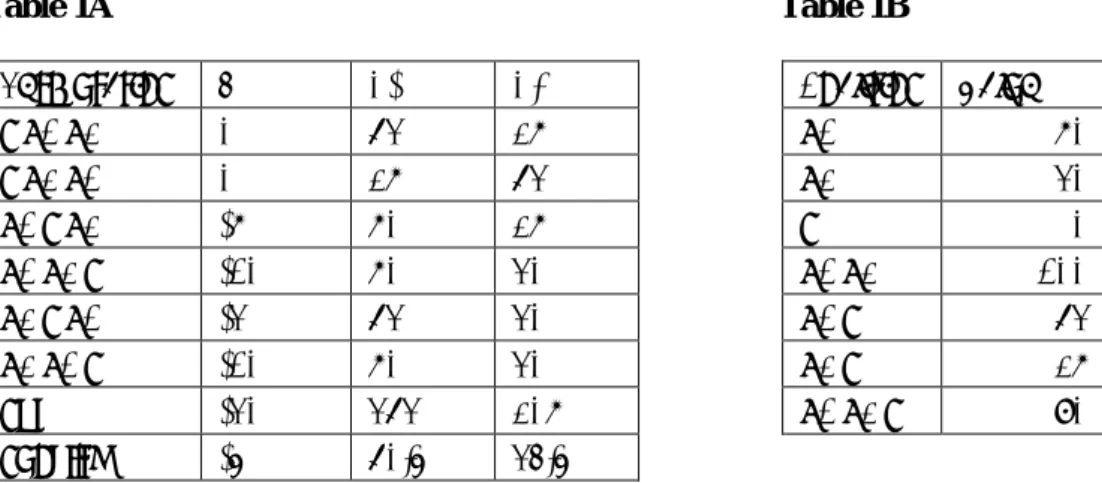
In order to illustrate the effects of emitter and receiver services, take the case of two business units, first with a receiver service, and then with an emitter service. The cost function for each is small enough to be defined in terms of a table of values of all possible coalition.
Table 1B shows the table of values for coalitions of a receiver service. The values of the two business units together is simply the sum of their stand-alone values. If the service joins either one of them, or both of them, in a coalition, the service is able to reduce their values by 10%. Table 1A shows the resulting Shapley analysis.
Table 1A Table 1B
Permutation S B1 B2 Coalition Value
S B1 B2 0 63 27 B1 70 S B2 B1 0 27 63 B2 30 B1 S B2 -7 70 27 S 0 B1 B2 S -10 70 30 B1 B2 100 B2 S B1 -3 63 30 B1 S 63 B2 B1 S -10 70 30 B2 S 27 Sum -30 363 207 B1 B2 S 90 Shapley -5 60.5 34.5
The Pro Rata allocations corresponding to the Shapley allocations in Table 1A are the stand-alone values v(B1) = 70 and v(B2) = 30. Both are greater than their corresponding Shapley values. The sum of Shapley values is equal to the value of the Grand Coalition, 90. The difference 10-90 = 10 represents the saving due to the service. In practice, this amount would be used for investment in the business. Perhaps it should be awarded to the service!
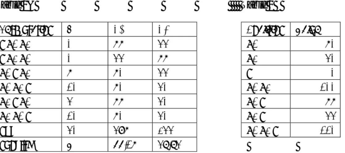
Tables 2A and 2B show the contrasting case of an emitter service. If the service joins either one of the business units or both of them in a coalition, the service increases their values by 10%. Effectively the service frustrates activities of the business unit(s).
Table 2A Table 2B
Permutation S B1 B2 Coalition Value
S B1 B2 0 77 33 B1 70 S B2 B1 0 33 77 B2 30 B1 S B2 7 70 33 S 0 B1 B2 S 10 70 30 B1 B2 100 B2 S B1 3 77 30 B1 S 77 B2 B1 S 10 70 30 B2 S 33 Sum 30 397 233 B1 B2 S 110 Shapley 5 66.17 38.83
This time the value of the Grand Coalition is 110, which is again equal to the sum of the Shapley values. Only B1 benefits from this arrangement in achieving a lower allocation than under Pro Rata allocation.
3.3.3 A Shapley analysis with n Business Units and one Service
We now extend and formalise the previous numerical cases to the general case of n (>1) business units and one service (i.e. n+1 players altogether). The result below is simple to state, but complex to prove.
Proposition 1
Consider n players B1, B2,…,Bn, who are business units, with respective values v1, v2,…,vn,, and a service S with zero value. Define a cost function implicitly by stating the values of coalitions, as in the group of equations (3). In (3), J is an indexing subset of the integers 1..n, and d is a real number in the range (0.1). v(Br) = vr, 1 ≤ r ≤ n v(S) = 0
J j j J j j v B v
J j j J j j d v B S v
1 (3)Then the Shapley values of the players S and Br (1 ≤ r ≤ n) are given by
n j j v d S SH 1 2 (4A)
r vj d B SH 2 2 1 ≤ r ≤ n (4B)d is termed the diversification factor and is typically 0.2 or less. A diversification factor measures the extent to which the service can influence the business units: typically 20% or less. If d > 0, the service is a receiver: SH(S) is negative. If If d > 0, the service is an emitter. SH(S) is positive. A proof is given in Appendix A. The result of this model is that the Shapley allocation of a player Br is simply its value modified a simple function of d. How to determine a value d will be addressed later in this paper.
As a check on the result, the sum of all allocations should be equal to the value of the grand coalition, which is (d+1)V. The sum of allocation is, using (4A) and (4B),
1
, asrequired. 2 2 2 2 2 2 ) ( 1 1 V d V d V d v d V d B SH S SH r n r n r r
In general, the idea of defining a standard way to treat the diversification value for all coalitions mirrors the approaches of Linhart et al (Linhart 1995), and Junqueira et al (Junqueira 2007).
3.3.4 Comparison with Pro Rata allocation
The Pro Rata allocations corresponding to Equation (4B) are given by equation (1). Since the service has value zero, PR(S) = 0, which corresponds to (4A).
The difference between the Shapley and Pro Rata allocations is then, from (1) and (4A)
0 that provided 0 ) ( ) ( 2 2 2 ) ( ) ( d B SH B PR dv v d v B SH B PR r r r r r r r (5)
On the other hand, for the service,
0 that provided 0 ) ( ) ( 2 0 ) ( ) ( d S SH S PR dV S SH S PR
Since S is a receiver service, the condition d < 0 applies. For BUs, the Pro Rata allocation clearly exceeds the Shapley allocation, which means that the task of explaining the allocation to managers of BUs is easy: their allocation is less than it might have been. The service has acquired a capital charge, which it passes on for reinvestment. Furthermore, no one player has been treated more favourably than any another. Note that without the diversification benefit, the Shapley and Pro Rata allocations would be equal. Besides, Pro Rata does not apply to departments that do not contribute to income, losses, etc., i.e. if a unit does not generate income then it would not be allocated capital.
3.3.5 Extension to two contrasting services
The subject matter of Proposition 1 was a group of n BUs with a single service. In this section we consider the case of two services: one emitter (service E) and one receiver (service R), with an interaction between the two services. Furthermore, the diversification factors for each service need not be equal. Let dE and dR be the respective diversification factors for the emitter and the receiver. From the viewpoint of the receiver service, the emitter service can be treated as the (n+1)th business unit. Therefore, using (4A),
R d v d V SH R n j j R 2 0 2 1
. (6A)Similarly, the emitter service sees the receiver as the (n+1)th business unit. Therefore, using (4A) again,
E d v d V SH E n j j E 2 0 2 1
. (6B)Each BU interacts with two services. Let the combined diversification factor, as experienced by each BU, be d’. To evaluate d’, we use the fact that the value of the Grand Coalition is equal to the sum of Shapley values of all players. The value of the Grand Coalition is, using equation (3), the sum of values of all players, multiplied by a factor (1+d’). Therefore
n j j E RV d V d v d d V 1 2 2 ' 2 2 ' 1 0 0 , from which d’ = dE + dR Therefore, from (4B)
j R E r v d d B SH 2 2 1 ≤ r ≤ n (6C)The result in equation (6C) illustrates the additive nature of games.
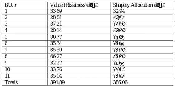
4 Application To Loss Data
In this section we apply the closed-form Shapley formulae (6A, 6B and 6C) to loss data for a collection of 11 BUs, each having sustained losses over the past five years. The receiver service (the “Risk department”) has moderated those losses, and an emitter service (the “IT department”) has worsened those losses by charging for its service. By noting total annual losses for each BU in discrete time periods, a loss correlation matrix, representing the dependency structure of the BUs, was calculated. The correlation matrix was used in conjunction with several copulas to calculate a correlated VaR loss value. The copulas considered were: Gaussian, Student-t, Gumbel, Clayton and Frank. The correlated VaR value was then compared with the VaR value derived from uncorrelated data. The overall diversification factor, d’, was the associated with the mean percentage reduction in VaR due to correlation over all copulas. The mean result was 4.47%, giving d’ = -0.0447. The factor used is negative since it represents an overall reduction in capital for the BUs.
The ‘riskiness’ values of the 11 BUs, and the value of the Grand Coalition, were obtained using empirical distribution parameters, and are listed in Table 3. The Shapley allocations, obtained using equation (6C) are shown alongside.
Table 3: Business Unit values
BU, r Value (Riskiness)(€m) Shapley Allocation (€m)
1 33.69 32.94 2 28.81 28.17 3 37.21 36.38 4 20.14 19.69 5 36.77 35.95 6 35.34 34.55 7 35.59 34.79 8 66.27 64.79 9 32.27 31.55 10 33.76 33.01 11 35.04 34.26 Totals 394.89 386.06
The difference 394.89 – 386.06 = 8.82 (€m) represents the net value of the Risk Department to the organisation as a whole.
In order to estimate the individual diversification factors dE and dR, it is necessary to estimate either the capital reduction due to the Risk Department, or the capital added by the IT Department. Ang and Straub (1998) estimate the charge for IT services to be in the range 15-20%, so we take the midpoint and set dE ~ 0.15. This gives dR ~ d’ - dE ~ -0.19. Then, using (6A) and (6B),
SH(R) ~ -38.4 (€m)
SH(E) ~ 29.6 (€m) (7)
The interpretation of the results in (7) is that the Risk Department reduces risk inherent in the BUs by about 10%, and the IT Department increases it by about 7.5%. Table 3 shows that each BU has a reduced capital relative to Pro Rata allocation.
The important question at this stage is "will this allocation be seen as fair by business units?". To answer this we can provide the following indicators.
All capital values are reduced.
No business unit can argue that any particular business unit is favoured over any other: they all have the same percentage capital reduction..
In order for services to survive, function properly and be of benefit to business functions (by reducing losses, costs and expenses), they should be allocated part of the total capital.
We stress that dominant new entrants to a coalition are not modelled in this analysis, where 'dominant' indicates that a new entrant has a more significant effect on a coalition than other players. The assumption throughout this analysis is that all players are equivalent in the way they add value to a coalition.
5 Conclusion
We have proposed an allocation methodology that is applicable to a large number of BUs, including two types of service: an emitter which increases capital payable by BUs, and a receiver which does the opposite. Using the Shapley method, we can account for diversification by considering coalitions. For the intended number of BUs (8-100), it is not feasible to do exact calculations for two reasons. First, the combinatorial complexity prevents it. Second, there is no standard way to calculate the value of a coalition. We therefore assume that all BUs contribute to a coalition in the same way, so that they each add their own value to the coalition when they enter it, provided that a service is not already in the coalition.. If it is, the sum of values of BUs in the coalition is multiplied by a diversification factor. This way of defining a cost function is open to modification or replacement as required, with the warning that Proposition 1 should be reworked if changes are made.
There are three principal results of this analysis.
1. The allocations of all UoMs decrease relative to their Pro Rata allocations, which makes the result acceptable to BU managers.
2. We have derived closed-form expressions for Shapley allocations, which can be used for a large number of UoMs, and take negligible computation time.
3. We have modelled a service as an entity that moderates the capital of UoMs by either absorbing capital from them or adding capital to them.
Appendix A
Proof of Proposition 1
B1, B2,…,Bn are n players who are business units, with respective values v1, v2,…,vn,, and S is a service with zero value. The values of possible coalitions are given by equations (3), as in the main text. J is an indexing subset of the integers 1..n, and d is a real number in the range (0.1).
v(Br) = vr, 1 ≤ r ≤ n v(S) = 0
J j j J j j v B v
J j j J j j d v B S v
1 (3)Then Then the Shapley values of the players S and Br (1 ≤ r ≤ n) are given by
J j j v d S SH 2 (4A)
r vj d B SH 2 2 1 ≤ r ≤ n (4B) ProofThe proof proceeds in three parts. First, by considering cases where S enters the coalition. This proves result (4A). Second, by considering cases where Bi enters before S, and third, where Bi enters after S. The second and third results together will give equation (4B).
Part 1: S enters the coalition
We consider cases where S is first to enter a coalition, then second, third and so on, up to last to enter. Let V = v1 + v2 +…+ vn
Consider the case where S is the rth member to enter the coalition. Then r-1 business units have entered prior to S and n-r+1business units will enter after S. Let J be the indexing set of the r-1 business units that entered before S, and let J’ be the indexing set of the remaining n-r+1 business units.
Then the marginal value attributed to S is
1 d
v v d v dV ) J j j J j j J j j
The number of occurrences for this value is the product of these parts: 1. (r-1)! permutations of the r-1 elements of J
3. n1Cr1 combinations of the r-1 elements of J.
Since there are (n+1)! permutations of the n+1 players, the Shapley value for the service, SH(S), is given by
2 2 ! 1 2 1 ! 1 ! 1 1 ! 1 ! 1 ! 1 ! 1 1 1 1 1 dV S SH n dV n n n dV S SH n r n n dV r n C r dV S SH n n r n r r n
(which is equation (4A) in the main text)
Part 2: Bi enters the coalition before S
Suppose that S is not already part of the coalition when Bi enters. Let J be the indexing set of the r-1 business units that entered before S (so that neither S nor Bi are indexed by J), and let J’ be the indexing set of the remaining n-r business units.
Then the marginal value attributed to Bi in this case is:
i J j j i J j j v v v v
The number of occurrences for this value is the product of these parts: 1. (r-1)! permutations of the r-1 elements of J (excluding Bi) 2. (n-r)! permutations of the n-r elements of J’(excluding Bi) 3. n1Cr1 combinations of the r-1 elements of J.
4. n-r+1 ways to place S among the elements of J’ The sum of marginals in this case for Bi, M1(Bi), is given by:
2 ! 1 1 2 ! 1 2 1 ! 1 1 1 ! 1 1 ! 1 ! 1 1 1 1 1 1
n v B M n v n n n v B M r n n v r n r n C r v B M i i i i i n r i n r r n i iPart 3: Bi enters the coalition after S
Suppose that S is already part of the coalition when Bi enters. J and J’ are defined as in Part 2. Then the marginal value attributed to Bi in this case is:
i J j j i J j j d v d v d v v d1
1 1
1 The number of occurrences for this value is the product of these parts: 1. (n-1)! ways to choose n-1 business units other than Bi
2. (r-1) ways to choose a slot for S, given that Bi is the rth to enter The sum of marginals in this case for Bi, M2(Bi), is given by:
2 ! 1 1 2 2 1 ! 1 1 1 ! 1 1 2 1 2
n v d B M n n n v d r n v d B M i i i n r i iAs in Part 1 there are (n+1)! permutations of the n+1 players. Therefore the Shapley value for Bi is given by:
2 2 2 ! 1 2 2 ! 1 1 2 ! 1 2 1 ! 1 i i i i i i i i v d B SH n d v n v d n v B M B M B SH n References
Ang,S and Straub,D. (1998) Production and Transaction Economies and IS Outsourcing:A Study of the U.S. Banking Industry. MIS Quarterly 22(4) 535-552
Aumann,R. and Shapley,L. Values of Non-Atomic Games. Princeton University Press (1974)
Butler,M. and Williams,H.P. The Allocation of Shared Fixed Costs. European Journal of Operational Research,
170 (2006)
Cambridge (2011) From Processes to Promise:How complex service providers use business model innovation to deliver sustainable growth. White paper, Cambridge Service Alliance. URL:
http://www.cambridgeservicealliance.org/uploads/downloadfiles/white%20paper%20processes%20to%20promi se.pdf
Castro,J., Gómez,D. and Tejada,J. Polynomial Calculation of the Shapley value based on Sampling. Computers and Operations Research, 36, 1726-1730, Elsevier (2009)
Dehez,P. Allocation of fixed costs: characterization of the (dual) weighted Shapley value. International Game Theory Review, 13(2), 141-157 (2011)
Garcia-Diaz, A. and Lee, D-J. Models for Highway Cost Allocation, ch. 6 in “Game Theory Relaunched", ed. Hanappi,H. INTECH (2013)
Magratta,J. (2002) Why Business Models matter. Harvard Business Review, May 2002
IBTimes (2013) RBS and Natwest Customers Suffer from Online Banking, ATMs, Debit Payments Outage URL: http://www.ibtimes.co.uk/rbs-online-banking-natwest-technical-glitch-computer-526843
Junqueira,M., da Costa,L., Barroso,L., Oliveira,G., Thomé,L. and Pereira,M. An Aumann-Shapley Approach to AllocateTransmission Service Cost Among Network Users in Electricity Markets. IEEE Transactions on Power Systems, 22(4) (2007)
Lai,R., Weill,P. and Malone,T. (2006) Do Business Models Matter? MIT. URL: http://seeit.mit.edu/Publications/DoBMsMatter7.pdf
Levitt, T. (1972) Production line approach to service, Harvard Business Review. 41–52.
Liben-Nowell,D., Sharp, A., Wexler, T. and Woods, K. Computing Shapley Value in Supermodular Coalitional Games. Computing and Combinatorics: Lecture Notes in Computer Science 7434, 568-579 (2012)
Linhart,P., Radner,R., Ramakrishnan,K. and Steinberg,R. The allocation of value for jointly provided services. Telecommunication Systems, 4,151-175 (1995)
Littlechild,S. and Owen,G. A simple Expression for the Shapley Value in a special case. Management Science,
20(3), Inst. of Management Science (1973)
Littlechild, S. and Thompson,G. Aircraft Landing Fees: A Game Theory Approach. The Bell Journal of Economics, 8(1) , 186-204, The RAND Corporation (1977)
Monti,F., Brunner,M., Piacenza,F. and Bazzarello,D. Diversification effects in operational risk: A robust approach. Journal of Risk Management in Financial Institutions, 3(3), 243-258. Henry Stewart (2010)
Press, W. H., Flannery, B. P., Teukolsky, S. A., and Vetterling, W. T. Cholesky Decomposition §2.9 (89-91), Numerical Recipes in FORTRAN: The Art of Scientific Computing. Cambridge University Press (1992)
Shafer,S.M., Smith,H.J. and Linder,J.C. (2005) The power of business models. Business Horizons 48, 199—207 Shapley, L A value for n-person Games. The Rand Corporation, (1953). Also in The Shapley value: Essays in
honor of Lloyd S. Shapley (ed. Roth,A.) CUP (1988)
Tarashev,N., Borio,C., and Tsatsaronis,K The systemic importance of financial institutions, in BIS Quarterly Review (page 77), Bank for International Settlements. (2009)