Capital deepening and non-balanced economic growth

Digitized

by

the

Internet

Archive

in

2011

with

funding

from

Boston

Library

Consortium

IVIember

Libraries

DEWEY

HB31

.M415

Massachusetts

Institute

of

Technology

Department

of

Economics

Working

Paper

Series

CAPITAL

DEEPENING

AND

NON-BALANCED

ECONOMIC

GROWTH

Daron

Acemoglu

Veronica

Guerrieri

Working

Paper

06-24

August

15,

2006

Room

E52-251

50

Memorial

Drive

Cambridge,

MA

021

42

This

paper can be

downloaded

without

charge from

the

Social

Science

Research Network

Paper

Collection at

MASSACHUSETTS

INSTITUTE

OF TECHNOLOGY

SEP

5 2005

Capital

Deepening

and Non-Balanced

Economic

Growth'*

Daron Acemoglu

Veronica

Guerrieri

MIT

University of

Chicago

First Version:

May

2004.

This

Version:

August

2006.

Abstract

This paperconstructs a model ofnon-balanced economic growth.

The

main economic

forceisthecombinationof differences in factorproportions andcapitaldeepening. Capital

deepening tends toincrease the relativeoutput ofthe sector witha greater capital share,

butsimultaneously induces a reallocation of capitaland labor away fromthat sector.

We

first illustrate this force using a general two-sector model.

We

then investigate it further

using a class of models with constant elasticity of substitution between two sectors and

Cobb-Douglas productionfunctions in each sector. In this class ofmodels, non-balanced

growth is shown to be consistent with an asymptotic equilibrium with constant interest

rateandcapitalshareinnationalincome.

We

alsoshowthat for realisticparametervalues,

the model generates dynamics that are broadly consistent with

US

data. In particular, the model generates more rapid growth of employment in less capital-intensive sectors,

more rapid growth of realoutput in more capital-intensive sectors sectors and aggregate

behavior inline withthe Kaldorfacts. Finally,

we

construct andanalyze amodelof

"non-balanced endogenousgrowth," which extendsthemainresults ofthepaperto aneconomy

with endogenous and directed technical change. This model shows that equilibrium will

typicallyinvolve endogenous non-balanced technological progress.

Keywords:

capital deepening, endogenous growth,multi-sector growth, non-balanced

economic growth.

JEL

Classification: O40, 041, O30.

'We thank John Laitner, Guido Lorenzoni, Ivan Werning and seminar participants at Chicago, Federal

ReserveBank ofRichmond, IZA,MIT,

NBER

EconomicGrowthGroup, 2005, Society ofEconomicDynamics,

Florence 2004and Vancouver2006, and Universitat ofPompeu Fabraforuseful comments and Ariel Burstein

for helpwiththe simulations. Acemoglu acknowledgesfinancial supportfromthe RussellSageFoundationand

1

Introduction

Most

models of economic growth strive to be consistent with the "Kaldor facts", i.e., the

relative constancy of the growth rate, the capital-output ratio, the share of capital

income

in

GDP

and

the real interest rate (see Kaldor, 1963,

and

also Denison, 1974,

Homer

and

Sylla, 1991, Barro

and

Sala-i-Martin, 2004).

Beneath

this balanced picture, however, are the

patterns that

Kongsamut,

Rebelo

and

Xie (2001)referto asthe "Kuznetsfacts",which concern

the systematic change in the relative importance ofvarious sectors, in particular, agriculture,

manufacturing

and

services (see Kuznets, 1957, 1973, Chenery, 1960,

Kongsamut,

Rebelo

and

Xie, 2001).

While

the Kaldor facts emphasize the balanced nature of economic growth, the

Kuznets

facts highlight its non-balanced nature. Figure 1 illustrates

some

aspects ofboththe

Kaldor

and Kuznets

facts for postwar US; the capital share of national income is relatively

constant, whereas relative

employment and

output in services increase significantly.^

The

Kuznets

facts have motivated a small literature,

which

typically starts by positing

non-homothetic preferences consistent with Engel's law.^ This literaturetherefore emphasizes

the demand-side reasons for non-balanced growth; the marginal rate ofsubstitution

between

different goods changes as an

economy

grows, directly leading to a pattern of

uneven

growth

between

sectors.

An

alternative thesis, first proposed

by

Baumol

(1967), emphasizes the

po-tentialnon-balanced natureofeconomicgrowthresultingfromdifferential productivity

growth

across sectors, but has received less attentionin the literature.^

This paper has two aims. First, it shows that there is a natural supply-side reason,

re-lated to Baumol's (1967) thesis, for economic

growth

to be non-balanced. Differences infactor

proportions across sectors (i.e., different shares of capital)

combined

with capital deepening

'AlldataarefromtheNationalIncome andProductAccounts (NIPA). Fordetailsanddefinitionsofservices,

manufacturing, employment, real

GDP

andcapitalshare, see AppendixB.

^See,forexample,Murphy, ShleiferandVishny(1989),Matsuyama(1992),Echevarria(1997), Laitner(2000),

Kongsamut,RebeloandXie(2001),Caselliand Coleman (2001), GoUin, Parente andRogerson (2002). Seealso

the interesting papers by Stokey (1988), Matsuyama (2002), Foellmi and Zweimuller (2002), and Buera and

Kaboski (2006), which derive non-homothetiticites from the presence of a "hierarchy ofneeds" or "hierarchy

of qualities". Finally, Hall and Jones (2006) point out that there are natural reasons for health care to be

a superior good (because expected lifeexpectancy multiplies utility) and show how this can account for the

increasein health carespending. Matsuyama (2005) presentsanexcellentoverviewof this literature.

Two

exceptions are thetworecentindependent papersbyNgaiandPissarides (2006) andZuletaandYoung

(2006). Ngai and Pissarides (2006), for example, construct a model ofmulti-sector economic growth inspired

by Baumol. In Ngai and Pissarides's model, there are exogenous Total Factor Productivity differences across

sectors, but all sectors have identical Cobb-Douglas production functions. While both of these papers eire

potentially consistent with the Kuznets and Kaldor facts, they do not contain the main contribution ofour

/

^^ ^^

^^ ,#

,# ^^ ^^

,# ,#

/

^^^-^ ^"^ ^'^

/

^"^^^^"'^^^^

^^

,c$^

_{^^ ,#}

,c# ,<#^^<:.^^c§?

I

-»-capitalshare-b-laborratioservicesovermanufacturing -*-realoutputratioservicesover manufacturing |

Figure 1: Capital share in national income

and

employment and

real

GDP

in services relative to manufacturing in the United States, 1947-2004. Source:

NIPA.

See text for details.

will lead to non-balanced growth.

The

reason is simple:

an

increase in capital-labor ratio will

raise output

more

in the sector with greater capital intensity.

More

specifically,

we

prove that

"balanced technological progress",^ capital deepening

and

differences in factor proportions

al-ways

causenon-balancedgrowth. Thisresult holdsirrespective ofthe exactsource ofeconomic

growth or the process of accumulation.

The

secondobjective ofthe paper is to present

and

analyze a tractable two-sector growth

model

featuring non-balancedgrowth

and

investigate under

what

circumstances non-balanced

growth can be consistent with aggregate Kaldor facts.

We

do this by constructing a class of

economies withconstant elasticityofsubstitution

between

two sectors

and Cobb-Douglas

pro-duction functions within each sector.

We

characterize the equilibria in this class ofeconomies withboth exogenous

and endogenous

technologicalchange.

We

show

that thelimiting

(asymp-*_"Balanced

technological progress" here refers to equal rates of Hicks-ncutra! technical change in the two

sectors. Hicks-neutral technological progress isboth a natural benchmark and also the typeof technological

totic) equilibrium takes a simple

form

and

features constant but different growthrates in each

sector, constant interest rate

and

constant share ofcapital in national income.

Other properties of the limiting equilibriumof this class of economies

depend on

whether

the products of the two sectors are gross substitutes or

complements

(meaning whether the

elasticity ofsubstitutionbetween theseproducts is greaterthan or lessthan one).

Suppose

for

this discussion that the rates of technological progress in the two sectors are similar. In this

case,

when

the

two

sectors are gross substitutes, the

more

capital-intensive sector dominates

theeconomy.

The

form ofthe equilibrium is

more

subtle

and

interesting

when

theelasticityof

substitution

between

these products is less than one; the growth rate of the

economy

is

now

determined by the

more

slowly growing, less capital-intensive sector. Despite the change in theterms oftrade against the faster growing, capital-intensive sector, inequilibrium sufficient

amounts

of capital

and

labor are deployed inthis sectorto ensurea fasterrate ofgrowth than

inthe less capital-intensive sector.

One

interestingfeatm^e is that our

model

economy

generates non-balanced growth without

significantly deviating from the Kaldor facts. In particular, even in the limiting equilibrium

both

sectors

grow

at positive (and unequal) rates.

More

importantly,

when

the elasticity of

substitution is less than one,^ convergence to this limiting equilibrium is typically slow

and

along the transition path, growth is non-balanced, while capital share

and

interest rate vary

by

relatively small amounts. Therefore, the equilibrium with an elasticity ofsubstitution less

than one

may

be able to rationalize

both

non-balanced sectoralgrowth

and

the Kaldor facts.

Finally,

we

present

and

analyzea

model

of"non-balancedendogenousgrowth," which shows

the robustness of our results to

endogenous

technological progress.

Our

analysis shows that

when

sectors differ in terms of their capital intensity, equilibrium technological change will

^Aswewillseebelow, theelasticityofsubstitutionbetweenproductswill belessthan oneifandonlyifthe

(short-run) elasticity ofsubstitutionbetweenlabor and capital isless thanone. Inviewofthe time-series and

cross-industry evidence, ashort-run elasticityofsubstitutionbetweenlabor and capital less than one appears

reasonable.

For example, Hamermesh (1993), Nadiri (1970) and Nerlove (1967) sm'vey arangeof early estimates ofthe

elasticityof substitution, whicharegenerallybetween0.3and0.7. David andVande Klundert (1965) similarly

estimate this elasticityto be inthe neighborhoodof0.3. Usingthe translog production function, Griffin and

Gregory (1976) estimateelasticitiesofsubstitutionfor nine

OECD

economiesbetween 0.06and 0.52. Berndt

(1976), onthe other hand, estimates an elasticity ofsubstitution equal to 1, but does not control for a time

trend, creatinga strong biastowards 1. Usingmore recent data, and various different specifications, Krusell,

Ohanian, Rios-Rull, and Violante (2000) and Antras (2001) also find estimates of theeleisticity significantly

lessthan1. Estimatesimplied bythe responseofinvestmenttothe user cost ofcapital alsotypicallyimplyan

elasticityofsubstitutionbetweencapitalandlaborsignificantly lessthan 1 (see, e.g., Chirinko, 1993, Chirinko,

itself be non-balanced

and

will not restore balanced growth

between

sectors.

To

the best of

ourknowledge, despite thelargehterature

on

endogenousgrowth, thereare

no

previous studies

that

combine

endogenoustechnological progress

and

non-balanced growth.^

A

variety of evidence suggests that non-homotheticitiesin

consumption

emphasized bythe

previousliteratureareindeed present

and

createatendency towards non-balancedgrowth.

Our

purpose in this paper is not to argue that thesedemand-side factors are unimportant, but to

propose

and

isolate

an

alternative supply-side force contributing to non-balanced growth

and

show

that it is potentially quite powerful as well. Naturally, whether or not our

mechanism

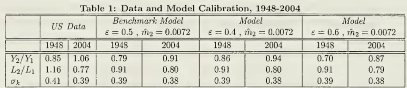
is

important inpractice is an empirical question. In Section 4,

we

undertake asimplecahbration

of our

benchmark model

to provide a preliminary investigation ofthis question.

As

a

prepa-ration for this calibration. Figure 2 shows the equivalent ofFigure 1, but with sectors divided

according to their capital intensity (see

Appendix

B

for details). This figure shows a

number

of important patterns: first, consistent with our qualitative predictions, there is

more

rapid

growth

of

employment

in lesscapital-intensive sectors.^ Second, alsoin linewith ourapproach,

thefigure

shows

that therate ofgrowth of real

GDP

isfasterin

more

capital-intensive sectors.

Notably, this contrasts with Figure 1,

which showed

faster growth-in,l)oth

employment and

real

GDP

forservices.

The

opposite

movements

of

employment and

real

GDP

forsectors with

high

and

lowcapital intensity is adistinctivefeature ofour approach (forthe theoretically

and

empirically relevant case ofthe elasticity of substitution less than one).

The

simple

calibra-tion exercise in Section4 also shows that our

model economy

generatesequilibrium

dynamics

consistent with both non-balanced growth at the sectoral level

and

the Kaldor facts at the

aggregate level. Moreover, not only the qualitative but also the quantitative implications of

our

model

appear to be broadly consistent with the data

shown

in Figure 2.

The

rest of the paper is organized as follows. Section 2 shows

how

the combination of

factor proportions differences and capital deepening lead to non-balanced growth. Section 3

constructs a

more

specific

model

with a constantelasticityofsubstitution

between

twosectors,

®See, among others, Romer (1986, 1990), Lucas (1988), Rebelo (1991), Segerstrom, Anant and Dinopoulos

(1990), Stokey (1991), Grossman and Helpman (1991a,b), Aghion and Howitt (1992), Jones (1995), Young

(1993). Aghion and Howitt (1998) and Barro and Sala-i-Martin (2004) provide excellent introductions to

endogenous growth theory. See also Acemoglu (2002) on models of directed technical change that feature

endogenous, but balanced technological progress in different sectors. Acemoglu (2003) presents a modelwith

non-balanced technologicalprogress betweentwosectors, but in the limiting equilibrium bothsectors growat

thesame rate.

^Note also that the magnitude ofchanges in Figure 2 is less than those in Figure 1, whichsuggests that

changes in thecomposition ofdemand between manufacturing and services are likelyresponsible forsome of

-f ^'5'"

^

^ ^

^

^ ^

^ ^

^ ^

^ ^

^V

^

^

^ ^ ^ ^ ^ ^

^

^

^

^

^

^

-_laborratiohigh relative tolowcapitalintensitysectors

-_{realoutputratiohighrelativetolowcapital intensitysectors}

Figure 2; Capital share in national income

and

eniployment

and

real

GDP

in high capital

.intensity sectors relative to low capital intensity sectors, 1947-2004. Source:

NIPA.

Cobb-Douglas

productionfunctions

and

exogenous technologicalprogress. It characterizesthe

full

dynamic

equilibrium of this

economy and

shows

how

the

model

generates non-balanced

sectoral growth, while remaining consistent with the Kaldor facts. Section 4 undertakes a

simple calibration ofour

benchmark

economy

to investigate whether the

dynamics

generated

by

the

model

areconsistent withthe changesintherelativeoutput

and

employment

of

capital-intensive sectors

and

the Kaldor facts. Section 5 introduces

endogenous

technological change

and shows

that ourgeneralresults continuetoholdinthepresenceofendogenous technological

progress acrosssectors. Section6 concludes.

Appendix

A

containsproofs thatarenotpresented

in thetext, while

Appendix

B

gives

some

details about

NIPA

data and sectoral classifications

2

Capital

Deepening

and Non-Balanced

Growth

We

first illustrate

how

differences in factor proportions across sectors

combined

with capital

deepening lead to non-balanced economic growth.

To

do this,

we

use a standard two-sector

competitive

model

withconstant returnsto scaleinbothsectors,

and two

factorsofproduction,

capital,

K,

and

labor, L.

To

highhght that the exact nature of the accumulation process is

not essential forthe results, in this section

we

take thesequence (process) of capital

and

labor

supplies,

[K

[t] ,

L

(i)]^Q, as given

and assume

that laboris suppliedinelastically. In addition,

we

omit explicit time

dependence

when

this will cause

no

confusion.

Finaloutput, Y, is produced as an aggregate oftheoutput of

two

sectors, Yi

and

I2,

Y^F{Yi,Y2),

and

we

assume

that

F

exhibitsconstant returnsto scale

and

istwicecontinuouslydifferentiable.

Output

in

both

sectors is

produced

with the production functions

Y,=A,Gi{KuLr)

(1)

and

Y2

=

A2G2iK2,L2).

(2)

The

functions

Gi

and

G2

also exhibit constant returns to scale

and

are twice continuously

differentiable.

Ai and A2

denote Hicks-neutral technology terms. Hicks-neutral technological

progress is convenient to

work

with

and

is also relevant since it is the type of

technolog-ical progress that the models in Sections 3

and

5 will generate.

We

also

assume

that F,

Gi and

G2

satisfy the Inada conditions; limp;.^q

dGj

{Kj,Lj)

/dKj

—

cx) for all Lj

>

0,

limL^^odGj{Kj,Lj)/dLj

=

00 for all

Kj

>

0, \imK^-,c<,dGj {Kj, Lj)

/dKj

=

for all

Lj

<

00, liuiL-^oo

dGj

{Kj,Lj)

/dLj

=

for all

Kj

<

00,

and

limVj_,o

dF

(Yi,Y2)jdYj

—

00

for all Yr^j

>

0,

where

j

=

1,2

and

~

j stands for "not j'\ These assumptions ensure interior

solutions

and

simplify the exposition, though they are not necessary for the results presented

in this section.

Market

clearing implies

K1

+

K2

-

K,

₍₃₎

where

K

and

L

are the (potentially time-varying) supplies of capital

and

labor, given

by

the

exogenous sequences

[K

{t),

L

{t)]'^Q.

We

take thesesequences to be continuosly differentiable

functions oftime.

Without

loss ofany generality,

we

also ignorecapital depreciation.

We

normalize the price ofthe final

good

to 1 in every period

and

denote the prices of Yi

and

I2 bypi

and

p2,

and

wage and

rentalrateof capital (interest rate)

by

w

and

r.

We

assume

that product

and

factor markets are competitive, so product prices satisfy pi

dFiYuY2)/dY,

P2

dF{Yi,Y2)ldY2

Moreover, given the Inada conditions, the

wage and

the interest rate satisfy:^

(4)

d

AiGijKuLi)

dA2G2{K2,L2)

_,,, ""

=

dL,

=

dL2

(^)

dAiGiiKi,Li)

_^

dA2G2{K2,L2)

^

dKi

dK2

Definition 1

An

equilibrium, given factorsupply sequences,

[K

it) ,

L

_(^)]^oi ^^ ^sequence of

product

and

factor prices, _{\p\ [t)}

,p2(t)

,w

(t),r(t)]^o ^^"^ factor allocations,

[Ki(i),

K2

(t),Li (t),L2 (0]~0' such that _(3), (4)

and

(5) are satisfied.

Let theshare of capital inthe two sectors be

0-1

=

—

—

_and

_a2

=

—--.

(6)

PiYi P2Y2 Definition 2 .

i Thereis capital deepening at time t ii

K

(t)

/K

(i)

>

L

{t)

/L

[t).

a

There arefactor proportion differences at timet if cti (f)

^

G2 it).

Hi Technological progress is balanced at time t if

Ai

(i)/Ai (t)

=

A2

(t)/A2 (i)

.

In this definition, ai (i) 7^ a2 (t) refers to the equilibrium factor proportions in the

two

sectors at time t. It does not necessarily

mean

that these will not be equal at

some

future

date.

The

next

theorem shows

thatifthereiscapitaldeepening

and

factorproportiondifferences,

then balanced technological progress is not consistent with balanced growth.

^WithouttheInada conditions, thesewould havetobewritten as

w

>

dAiGi{KuLi)/dLi and Li

>

0,

Theorem

1

Suppose

that at time t, there are factor proportion differences

between

the

two

sectors, technological progress is balanced,

and

there is capital deepening, then growth is not

balanced, that is, Yi (t)/Yi (t) 7^Y2 (t)/Y2(t).

Proof.

First define the capital to labor ratio inthe two sectors as

fci

=

-tr-

and

k2

=

-y-,

Li

L2

and

the "per capitaproduction functions" (without the Hicks-neutral technologyterm) as

_

G'i(Xi,Li)

G2{K2,L2)

,_.

5i(fci)

=

_T

and

52(^2)

=

z •

(7)

Li

L2

Since

Gi

and

G2

are twice continuously differentiable, so _{are gi}

and

52-Now,

differentiating the production functions for the two sectors.

and

Y2

A2

K2

, , 1/9

Y2-A2^'''^-K2^^'-'''^T2

Suppose, to obtain a contradiction, that Yi/Y\

=

Y2/Y2. Since

A\IA\

—

A2/A2

and

cti

^

0-2,

this implies ki/ki

^

^2/^2- [Otherwise, k\lk\

—

^2/^2

>

0,

and

capital deepening implies

Yi/Yi

^

Y2/Y2; for example, ifai

<

cto, then

Y/Yi

<

Y2/Y2].

Since

F

exhibits constant returns to scale, (4) implies

^

=

^

=

0. ₍₈₎

Pi P2

Given the definition in (7), equation (5) yields the following interest rate

and

wage

condi-tions: r

=

PiAig[iki) (9)

=

P2^252(^2) ,

and

w

=

PiAi{gi{ki)-g[{ki)ki)

(10)

=

P2A2

(52(^2)

-

92

{h)

^2) •

Differentiating the interest rate condition, (9), with respect to time

and

using (8),

we

obtain:

where

_

g'l(fci) fci ,

_9JM^

E„i

=

—

, ,, ,

and

e„'

=

—

, ,, . .

Since

AijAi

=

A2/A2,

Differentiating the

wage

condition, (10), with respect to time, using (8)

and

some

algebra

gives:

Ai

(71 ki

_

A2

(T2 ^2

Since

Ai/Ai

=

^2/^42

and

ai 7^ CT2, this equation is inconsistent with (11), yielding a

contra-diction

and

provingthe claim.

The

intuition for this result can be obtained as follows.

Suppose

that there is capital

deepening

and

that, for concreteness, sector 2 is

more

capital-intensive (i.e., o"i

<

a2).

Now,

if

both

capital

and

labor are allocated to the

two

sectors with constant proportions, the

more

capital-intensive sector, sector 2, will

grow

faster than sector 1. In equilibrium, the faster

growth insector 2 willnaturally changeequilibriumprices,

and

thedecline intherelativeprice

ofsector 2will cause

some

ofthe labor

and

capital tobe reallocated to sector 1. However, this

reallocation cannot entirelyoffset the greater increase inthe outputofsector2, since, if it did,

therelative price change that stimulated thereallocation

would

not take place. Consequently,

equilibrium growth

must be

non-balanced.

The

proof of

Theorem

1 also

makes

it clear that balanced technological progress is not

necessaryfortheresult,but simplysufficient. Thispointisfurtherdiscussed following

Theorem

3 in the next section.

It is useful to relate

Theorem

1 toRybczynski's

Theorem

in internationaltrade

(Rybczyn-ski, 1950). Rybczynski's

Theorem

states that for an

open

economy

within the "cone of

di-versification" (where factor prices do not

depend on

factor endowments), changes in factor

endowments

will be absorbed

by

changes in sectoral output mix.

Our

result can be viewed

as a closed-economy analogue of Rybczynski's

Theorem;

it shows that changes in factor

even

though

relativepricesofgoods

and

factorswill changein response to the changein factor

endowments.^

Finally,theproofof

Theorem

1

makes

it clearthatthe two-sector structureisnot necessary

forthis result. In light ofthis,

we

alsostate ageneralizationforA'^

>

2 sectors,

where

aggregate

output is given

by

the constant returns to scale production function

Y^F{Yi,Y2,...,Yn).

Defining Uj as the capital shareinsector j

—

1,...,N as in (6),

we

have:

Theorem

2

Suppose

that at time t, there are factor proportion differences

among

the A''

sectors inthe sense that thereexistsi

and

j

<

N

suchthatctj {t)

^

Uj (f), technological progress

is balanced

between

i

and

j, i.e., Ai (i)/Ai{t)

—

Aj

{t)/Aj(i),

and

there is capitaldeepening,

i.e.,

k

(t)

jK

(t)

>

L

(t)

/L

{t), then growth is not balanced

and

Y

(i)/Fj [t] j^ Yj {t)/Yj (t).

The

proofof this

theorem

parallels that of

Theorem

1

and

isomitted.

3

Two-Sector

Growth

with

Exogenous

Technology

The

previous section demonstrated that differences in factor proportions across sectors

and

capital deepening will lead to non-balanced growth. This result

was

proved for a given

(ar-bitrary) sequence of capital

and

labor supplies,

[K

(t) ,

L

{t)]^Q, but this level of generality

does not allow us to fully characterize the equilibrium path

and

its limiting properties.

We

now

wish to analyze the equilibrium behavior of such an

economy

fully,

which

requires us to

endogenize thesequence ofcapitalstocks (so that capital deepeningemerges as an equilibrium

phenomenon).

We

will accomplish this

by

imposing

more

structure

both on

the production

technology

and

on preferences. Capital deepening will result from exogenous technological

progress,

which

will in turnbe endogenized in Section 5.

^Note also that even ifthe result in Theorem 1 holds asymptotically {as t —^ oo), it does not contradict

the celebrated "Turnpike theorems" in the optimal growth literature (e.g., Radner, 1961, Scheinkman, 1976,

Bewley, 1982,McKenzie, 1998, Jensen, 2002). Thesetheoremsshowthat starting from differentinitialpoints,

theeconomywilltendto thesameasymptotictrajectory. Thefactthatgrowthisnon-balanced does notpreclude

this possibility.

3.1

Demographics,

Preferences

and

Technology

The

economy

consists of

L

{t) workers at time t, supplying their labor inelastically.

There

is

exponential population growth,

L{t)

=

exp{nt)

L

(0)

.

(12)

We

assume

thatallhouseholdshaveconstantrelative riskaversion

(CRRA)

preferences over

total household

consumption

(rather thanper capitaconsumption),

and

allpopulation growth

takes placewithinexistinghouseholds (thus thereis no growthinthe

number

ofhouseholds).^°

This implies that the

economy

admits a representative agent with

CRRA

preferences:

where

C

{t) is aggregate

consumption

at time t, _p is the rate of time preferences

and

9

>

Q

is the inverse of the intertemporal elasticity of substitution (or the coefficient ofrelative risk

aversion).

We

again drop time arguments to simplify the notation

whenever

this causes

no

confusion.

We

also continue to

assume

that there is no depreciation of capital.

The

flow budget constraint for the representative

consumer

is:

k

= rK

+

wL +

I[-C.

(14)

Here

w

is the equilibrium

wage

rate

and

r is the equilibrium interest rate,

K

and

L

denote

the total capital stock

and

the total labor force in the economy,

and

IT is total net corporate

profits received

by

the consumers (which will be equal to zero in this section).

The

uniquefinal

good

is produced by combiningthe output of

two

sectorswith

an

elasticity

ofsubstitution e

e

[0,oo):

Y

=

_7^1 ^

+

(1-7)^^2" ₍₁₅₎

where 7

is a distribution parameterwhich determinestherelative importanceofthe two goods

inthe aggregate production.

The

resource constraint ofthe economy, in turn, requires

consumption

and

investment to

be lessthan totaloutput,

Y

= rK + wL +

11, thus

k

+

C

<Y.

(16)

^ _Thealternative would betospecify population growth takingplaceat the extensivemargin, in which case

the discount rate of the representativeagentwould be p

—

n rather thanp, without any important changesin

theanalysis.

The

two goods Yi

and

Y2 are produced competitively using constant elasticityof

substitu-tion

(CES)

production functions with elasticity ofsubstitution

between

intermediates equal to

z/> 1:

^^1 .,_, \ IJ^ / /M2 ^_j

n=(/

yiii)

—

di\

andy2=(/

y2{i)

—

di\ , (17)

where

2/i(i)'s

and

2/2(O's denote the intermediates in the sectors that have different

capi-tal/labor ratios,

and

Mi

and

M2

represent the technology terms. In particular

Mi

denotes

the

number

of intermediates in sector 1

and

M2

the

number

ofintermediate goods in sector

2. This structure is particularly useful since it can also be used forthe analysis ofendogenous

growth in Section 5.

Intermediate goods are produced with the following

Cobb-Douglas

technologies

yi{i)

=

/i(z)"'fci(i)'""^

and

ya(i)

=

h

{if

h

_W'""'

,

(18)

where

_h

(i)

and

fci(i) are labor

and

capital used in the production of

good

i ofsector 1

and

I2 (i)

and

k2 (i) are labor

and

capital used in the production of

good

i ofsector 2.-^^

The

parameters aj

and

02 determine which sector is

more

"capital intensive".'^

When

ai

>

a2, sector 1 is lesscapital intensive, while the converse applies

when

ai

<

0:2. Intherest

ofthe analysis,

we

assume

that

ai

>

a2, (Al)

which

only rules out the case

where

ai =0:2, since the two sectors are otherwise identical

and

the labeling of the sector with the lower capital share as sector 1 is without loss of any

generality.

All factor markets are competitive,

and market

dealing for the

two

factors imply

/Ml rM2 / li{i)di+ l2{i)di

=

Li

+

L2^L,

(19) JO Jo

and

Ml f-M2 ki{i)di+ k2{t)di

=

Ki

+

K2

=

K,

(20) Jo

'^Strictly speaking, we shouldhavetwoindices, i\ e

Mi

and 12€

M2,

where

Mj

istheset ofintermediates

oftypej, and

Mj

isthemeasureofthe set Mj.

We

simphfy thenotationbyusingagenericito denoteboth

indices,and letthecontext determine which indexis beingreferredto.

'^We use the term "capital intensive" as corresponding to a greater share of capital in value added, i.e.,

(72

>

ci in terms ofthe notation of the previoussection. Wliile this share is constant because ofthe

Cobb-Douglas technologies,theequilibrium ratiosof capital tolaborin thetwosectors depend onprices.

where

the first set of equalities in these equations define Ki,L-[,

K2

and

L2 as the levels of

capital

and

labor used in the

two

sectors,

and

the second set of equalities impose market

clearing.

The number

of intermediategoods in the two sectors evolve at the exogenous rates

—

_—

=

mi

and

—

-—

=

mo. (21)

Ml

M2

Since

Mi

and

M2

determine productivity in their respective sectors,

we

will refer to

them

as

"technology". Inthis section,

we

assume

that allintermediates are alsoproduced competitively

(i.e., any firm can produce

any

of the existing intermediates). In Section 5,

we

will modify

this assumption

and assume

that

new

intermediates are invented

by

R&D

and

the firm that

invents a

new

intermediate has afully-enforced perpetual patent for its production.

3.2

Equilibrium

Recall that

w

and

r denote the

wage and

the capital rental rate,

and

pi

and

p2 denote the

prices ofthe Yi

and

Y2 goods, with the priceofthe final

good

normalizedto one. Let [9i(i)]j=i

and

_[92(2)]i=\ be the prices for labor-intensive

and

capital-intensiveintermediates.

Definition 3

An

equilibrium is given

by

paths forfactor, intermediate

and

final goods prices

r, w, [qi{i)]^\ , [q2{i)]fi\ , Pi

and

p2,

employment and

capital allocation [li{i)]fi\, [l2{i)]^i

,

[ki{i)]^J^^I [^2(j)]j=:^i such that firms

maximize

profits

and

markets clear,

and consumption and

savings decisions,

C

and

K,

maximize consumer

utility.

It isuseful tobreak the characterization of equilibriuminto

two

pieces: static

and

dynamic.

The

staticpart takes the state variables ofthe economy,

which

are thecapital stock, the labor

supply

and

the technology,

K,

L,

Mi

and

M2,

asgiven

and

determinesthe allocation of capital

and

labor across sectors

and

factor

and good

prices.

The

dynamic

part of the equilibrium

determines the evolution of the endogenous state variable,

K

(the

dynamic

behavior of

L

is

given

by

(12)

and

those of

_Mi

and

M2

by (21)).

Our

choice ofnumeraireimplies that the price ofthe final good, P, satisfies:

i^P=[Yp\'-^+{i-^rpl

£„!"£!ITi

Next, since Yi

and

Y2 are supplied competitively, their prices are equal to the value of their

marginal product, thus

Pi=7(y)

'

and

_p2

=

₍₁

-7)

(y

)

\

(22)

and

the

demands

forintermediates, yi{i)

and

j/2(i), are given

by

the famiharisoelastic

demand

curves:

^=f#V'

and

Ml^fMOy'.

(23)

Since all intermediates are

produced

competitively, prices

must

equalmarginal cost.

More-over, given the production functions in (18), the marginal costs of producing intermediates

take the familiar

Cobb-Douglas

form,

mci

(i)

=

ap'

(1

-

ai)"'-^r^-^'^w"'

and

mc2

(i)

=

aj"^

(1

-

aa)"'"^r^-^^w''^

Therefore, at all points in time, intermediateprices satisfy

qi{i)

=

ai{l-ai)'''-\^-^'w°\

(24)

and

q2{i}=a2{l-a2f'-^r^~"^w''\

(25)

for all i.

Equations (24)

and

(25) imply that all intermediates in each sector sell at the

same

price 9i

=

9i(0 for all i

<

Ml

and

₉₂

=

₉₂(^) for all i

<

M2.

This

combined

with (23) implies that the

demand

for,

and

the production of, the

same

type ofintermediatewill be the same. Thus:

yi{i)

=

h{i)'''h{i)'-^'

=

/^^ifcj-"!

_=yi

_•\fi<Mi

2/2(0

-

l2{ir-k2{i)'-'''

=

l^^kl''^^

=y2

yi<M2,

where

li

and

fci are the levels of

employment and

capital used in each intermediate of sector

1,

and

I2

and

k2 are the levels of

employment and

capital used for intermediates in sector 2.

Market

clearing conditions, (19)

and

(20), then imply that

h

—

Li/Mi,

k\

—

Ki/M\,

h =

L2/M2

and

/c2

—

K2/M2,

so

we

have theoutput ofeach intermediate in the twosectors as

y\

=

.}

and

2/2

=

^

J

. ₂₆₎

^

Ml

^

M2

Substituting (26) into (17),

we

obtain thetotal supplyoflabor-

and

capital-intensivegoods

as

Yi

^

M{^

L^'

kI'"' and

Y2

=

M^'

L'^U<l-''\ (27)

Comparing

these (derived) productionfunctions to ₍₁₎

and

(2) highlightsthat in thiseconomy, the production functions

Gi and

G2

from

the previous section take

Cobb-Douglas

forms,

with one sector always having a higher share of capital than the other sector,

and

also that

1 1

Ai

=

M{-'

and

A2

=

M{-'

.

In addition, combining (27) with (15) implies that the aggregateoutput ofthe

economy

is:

Y

7

I

Mr'

L^U<1-^')

'

₊

(1

-

7)

(m/-'

L^-K^-^^

(28)

Finally, factor prices

and

the allocation of labor

and

capital

between

the two sectors are

determined by:^^

-=(l-7)a2g)'g

(30)

.

=

7(l-..)(^)'^

(31)

r

=

_{(l-7)(l-a2)(^)'f.}

(32)

These

factor prices takethe familiarform, equal tothe marginalproductofafactor from (28).

3.3

Static

Equilibrium:

Comparative

Statics

Letus

now

analyze

how

changesinthestate variables, L,

K,

Mi

and

M2,

impact

on

equilibrium

factor prices

and

factor shares.

As

noted in the Introduction, the case with £

<

1 is ofgreater

interest (and empirically

more

relevant as pointed out in footnote5), so, throughout,

we

focus

on

this case (though

we

give the result for the case in which e

>

1,

and

we

only omit the

standard case with e

=

1 to avoid repetition).

^ _{Toobtainthese equations,startwith the cost functions above,and derivethe demandforfactors byusing}

Shepherd'sLemma. Forexample,forthe sector 1,these are/i

=

(ifj, ^) yi and fci

=

( i°)^

~

)

yi-Combinethesetwoequations to derive theequiUbriumrelationshipbetweenrandw. Then usingequation (24),

eliminate r to obtain arelationship between

w

and gi. Finally, combining this relationship withthe demand

curvein (23),themarketclearing conditions, (19) and (20), andusing (27) yields (29). Theotherequations are

obtainedsimilarly.

Let us denote the fraction of capital

and

labor

employed

in the labor-intensive sector

by

K

=

K\/

K

and

A

=

Li/L

(clearly I

—

k

=

K2/K

and

1

—

A

=

L2/L).

Combining

equations

(29), (30), (31) and (32),

we

obtain:

n

=

1

-ai\

[I

-7^

(Yi

«iy

V

7

J

\Y2

and

1

—

ai\

(ot2\

/I

A

=

+

1 (33) (34) 1

—

a2/\ai/\

K

Equation (34)

makes

it clear thatthe share oflabor in sector 1, A, is monotonically increasing

in the share of capital in sector 1, k.

We

next determine

how

these two shares change with

capital accumulation

and

technological change.

Proposition

1 In equilibrium,

1.

d\nK

dluK

(1

—

e) (a-i

—

ao) (1

—

k) „ , s, n „ /„_s

dhiK

d\nL

1

+

(1

-

s) (ai

-

02) (k

-

A) ^ '^ ' ^ '

d\Q.K

dlnK

{\

—

e){\

—

k)_liy

—

\)

d\nM2

^^dhiMi

"

l

+

(l-£)(ai-a2)(K-A)

^

'

^ ^

The

proofof this proposition is straightforward

and

is omitted.

Equation (35), part 1 ofthe proposition, statesthat

when

the elasticityofsubstitution

be-tween sectors, e, is less than 1, the fraction of capital allocated to the capital-intensive sector

declines in the stock of capital (and conversely,

when

e

>

1, this fraction is increasing in the

stock ofcapital).

To

obtain the intuitionforthis comparativestatic,

which

is useful for

under-standing

many

ofthe results that will follow, note that if

K

increases

and k

remains constant,

thenthe capital-intensive sector, sector 2, will

grow by

more

thansector 1. Equilibrium prices

given in (22) then imply that

when

e

<

1 therelative price ofthe capital-intensive sectorwill

fall

more

than proportionately, inducingagreaterfraction of capital to be allocatedtothe less

capital-intensive sector 1.

The

intuition for the converse result

when

e

>

1 is straightforward.

Moreover, equation (36) impliesthat

when

the elasticityof substitution, e, is lessthanone,

an

improvement

in the technology of a sector causes the share of capital going to that sector

to fall.

The

intuitionis again the same:

when

e

<

1, increased production in a sector causes

a

more

than proportional decline in itsrelative price, inducing a reallocation ofcapital

away

from it towards the other sector (againthe converse results

and

intuition apply

when

e

>

1).

Proposition 1 gives only the comparative statics for k. Equation (34) immediately implies

that the

same

comparative statics apply to A

and

thus yields the following corollary:

Corollary

1 In equilibrium, 1. din A din A 2. din A din A

>

<=>£<

1.

dlnM2

dlnMi

Next, combining (29)

and

(31),

we

also obtain relative factor prices as

w

ai _{f K,K'}

r

l-ai\XLj'

and

the capital share in the

economy

as:''^

(37) c-l

tK

^ _

fYr\

-^_i aic

=

-^

= l-7a'i(^)

X'\

(38)

Proposition

2 In equilibrium, 1. dIn[w/r) dIn[w/r) 1

dlniC

dlnL

1

+

(1

-

e)(qi

-

02) (k

-

A) 2.

d\n[w/r)

d\T\{w/r) (1

-

s) («;

-

A)/(i^

-

1)

>0.

dlnM2

dlnMi

1

+

(1

-

e) (ai

-

02) (k

-

A)

dlna;<-<

<^ (ai

-

a2)(1

-

e)

>

0.

d\xiK

dIn

_UK

dIn

_uk

dlnM2

~

dlnMi

<

^

e

<

1. ₍₃₉₎

<

<^ (ai

-

02)

{l-e)>

0. (40)

^''Notethat

ok

refers tothe share of capital innational income,andis thusdifferentfromthe capital shares

inthe previoussection, which weresector specific. Sector-specific capitalshares are constant here becauseof

theCobb-Douglasproduction functions (inparticular, a\

=

ai and a2

=

Proof.

Parts 1

and

2 follow from differentiating equation (37)

and

Proposition 1.

Here

we

prove parts 3

and

4. First,

combine

the production function

and

the equilibrium capital

allocation to obtain -1

7

+(1-7)

7

1

+

1 1

-

"2,

Then, using the results ofProposition 1

and

the definition of

_gk

from (38),

we

have:

dXxvoK

_n(^^^K\

(^

—

0L\\ (\

—

e) {q.\

—

OL-i) {\

—

k) I K

dhiK

CTR

02/1

and

where

dIn

aK

dIn(7A'

d\nM2

din

Ml

=

S

1

—

<^k\

f^

—

C(.\ C^K 1

-

e)(ai

-

0:2){k

-

x)

\-

ai)

1

+

(1

-

e)(ai

-

02) (k

-

x) ' (41) (42)

S

=

\

—

a.\ a'2

-1

1

—

Q'l

1-0:2

1

-

-1

K

Clearly,

5

<

<=> _Qi

>

a2.

Equations (41)

and

(42) then imply (39)

and

(40).

The

most

important result in this proposition is part 3, which links the equilibrium

rela-tionship

between

the capital share in national income

and

the capital stockto the elasticityof

substitution. Sincea negative relationship betweenthe share of capital innational income

and

the capital stockis equivalent to capital

and

labor being gross

complements

in the aggregate,

this result also implies that, as claimed in footnote 5, the elasticity ofsubstitution between

capital

and

labor is lessthan one if

and

only ife is less than one. Intuitively, as in

Theorem

1,

an

increase inthe capital stockofthe

economy

causes the output ofthe

more

capital-intensive

sector, sector 2, to increase relative to the output in the less capital-intensive sector (despite

thefact that theshareof capital allocatedtotheless-capital intensivesector increases as

shown

in equation (35)). This thenincreases the productionofthe

more

capital-intensive sector, and,

when

£

<

1, it reduces the relative reward to capital (and the share of capital in national

income).

The

converse result applies

when

e

>

1.

Moreover,

when

e

<

1, part 4 implies that an increase in

M\

is "capital biased"

and

an

increase in

M2

is "labor biased".

The

intuition for

why

an

increase in the productivity ofthe

sector that is intensive in capital is biased towardlabor (and vice versa) isonce again similar:

when

the elasticity ofsubstitution between the

two

sectors, e, is less than one, an increase in

theoutputofasector (thistime driven

by

achangeintechnology) decreases itsprice

more

than

proportionately, thus reducingtherelative compensationofthe factor used

more

intensively in

that sector (see

Acemoglu,

2002).

When

£

>

1,

we

have theconverse pattern,

and

an increase

in

M2

is "capital biased," while

an

increase in

_Mi

is "labor biased"

3.4

Dynamic

Equilibrium

We

now

turn to the characterization of the

dynamic

equilibrium path of this economy.

We

startwith theEuler equationforconsumers, whichfollows fromthemaximizationof(13).

The

Euler equation takes the familiar form:

§

=

^(r-p).

(43)

Since the onlyassetofthe representativehouseholdin this

economy

iscapital,thetransversality

condition takes the standard form:

" "^

Hm

K(i)exp(-/ r(r)dTj

-=0, (44)

which, togetherwith the Euler equation (43)

and

the resource constraint (16), determines the

dynamic

behavior of

consumption

and

capital stock,

C

and

K.

Equations (12)

and

(21) give

thebehavior of L,

M\

and M2.

We

can therefore define a

dynamic

equilibrium as follows:

Definition

4

A

dynamic

equilibrium is given by paths of wages, interest rates, labor

and

capital allocation decisions, w, r, A

and

k, satisfying _{(29), (30), (31), (32),} (33)

and

(34),

and

of consumption, C, capital stock,

K,

employment,

L,

and

technology,

Mi

and

M2,

satisfying

(12), (16), (21), (43),

and

(44).

Let us also introduce the following notation for growth rates of the key objects in this

economy: Li L2

L

-T

=

ni, -r-

=

n2,

_y

=n,

Lil 1^2 -^

ki

_

i<2

_

k

_{_}

—

=

Zl,

—

^

Z2,

-

=

Z, 19

Yx

_

Y2

_{_}

Y

_{_}

-=5i, -=52,

^=5,

so that Us

and

Zg denote the

growth

rate oflabor

and

capital stock, nis denotes the growth

rate of technology,

and

Qs denotes the growth rate ofoutput in sector s. Moreover,

whenever

they exist,

we

denote the corresponding asymptotic growth rates

by

asterisks, i.e.,

n*

=

lim Us , zl

=

lim Zs

and

g^

—

lim gg.

t—tOO t—too t—KX>

Similarly denote the asymptotic capital

and

labor allocation decisions

by

asterisks

K*

—

lim

K

and

A*

—

lim A.

t—>oo t—>oo

We

now

state

and

prove

two

lemmas

that will be useful both in this section

and

again in

Section 5.

Lemma

1 Ife

<

1, then ni

_^

n2 •<=> 2:1

^

22 "^ 5i

_^

52 Ife

>

1, then ni

_^

n2 -^ zi

_^

Z2

«

91

_I

52-Proof.

Differentiating (29)

and

(30) with respect to time yields

w

le-1

^

w

l£-l

,^^,

—

+

ni

=

-5

H gi

and

—

+

712

=

-5

H 52- (45)

w

e e

w

£ e

Subtracting the second expression

from

the first gives ni

—

n2

—

(e

—

1)(51

—

52)/e,

and

immediately implies the first part ofthe desired result. Similarly differentiating (31)

and

(32) yields

r 1 £

—

1 ,7- 1 e

-I

_,,„,

-

₊

21

=

-5

H 51

and -

+

22

=

-5

+

52- (46)

r £ e r

be

Subtracting the second expression from the first again gives the second part ofthe result.

This

lemma

establishes the straightforward, but atfirst counter-intuitive, result that,

when

the elasticity ofsubstitution

between

the two sectors is less than one, the equilibrium growth

rate ofthe capital stock

and

labor force in the sector that is growing faster

must

be Itss than

in the other sector.

When

theelasticity ofsubstitution isgreater than one, the converse result

obtains.

To

see the intuition, note that terms oftrade (relative prices) shift in favor of the

more

slowly growing sector.

When

the elasticity of substitution is less than one, this change

in relative prices is

more

than proportional with the change in quantities

and

this encourages

more

ofthe factors to be allocated towards the

more

slowly growing sector.

Lemma

2

Suppose

the asymptotic growth rates _g^

and

§2 exist. If e

<

1, then g*

=

min{5i*,5^}.

lie>l,

then g*

^

max

_{gl,g^}.

Proof.

Differentiating the production function for the final

good

(28)

we

obtain:

(47)

7^1 ^ ₅₁

+

₍₁

-7)^2 ' ₅₂

jY,^

+(l-7)i^2^

This equation,

combined

with e

<

1, imphes that as i

—

>• oo, g*

=

min{gj',p2}- Similarly,

combined

withe

>

1, it implies that as i

—

>oo, 5*

=

max

_{^J^,

52}-Consequently,

when

the elasticity ofsubstitution isless than 1, the asymptoticgrowthrate

of aggregate output will be determined

by

the sector that is growing

more

slowly,

and

the

converse applies

when

e

>

1.

3.5

Constant

Growth

Paths

We

first focus

on

asymptotie^equilihriura paths, which are equilibrium paths that the

economy

tends to as t

^

00.

A

constant growth path

(CGP)

is defined as an equilibrium path

where

the asymptotic growth rate of

consumption

exists

and

is constant, i.e.,

hm

7:7

=

5c-From

the Euler equation (43), this also implies that the interest rate

must be

asymptotically

constant, i.e., limt_,oo'^

=

0.

To

establishthe existence ofa

CGP, we

impose the following parameter restriction:

p>-

-max*^

—

i,-^

^

+

(l-6')n. (A2)

1/

—

1

[dl

Oi2

}

This assumption ensures that the transversahty condition (44) holds.'^

_Terms

_{of the form}

mi/ai

or 1112/02 appear naturally in equilibrium, since they capture the "augmented" rate

oftechnological progress. In particular, recall that associated with the technological progress,

there will also be equilibrium capital deepening in each sector.

The

overall effect on labor

productivity (and output growth) will

depend on

the rate oftechnological progress

augmented

^^If insteadwetook the discount rateofthe representativehousehold tohe p

—

n as noted in footnote 10,

thennin (A2) would not bemultipliedby (1 —6).

with the rate ofcapital deepening.

The

terms

mi/ai

or 1712/00 capture this, since a lower ai

or a2 corresponds to a greater share of capital inthe relevant sector,

and

thus a higher rate of

augmented

technological progressfora given rateofHicks-neutral technological change. Inthis

light,

Assumption

A2

can

be

understood as implyingthat the

augmented

rateoftechnological

progress should be low

enough

to satisfy the transversality condition (44).

The

next

theorem

isthe

main

resultof thispartofthepaper

and

characterizestherelatively

simple form of the

CGP

in the presence ofnon-balanced growth.

Although

we

characterize a

CGP,

in the sense that aggregateoutput growsata constant rate, it is noteworthy that growth

is non-balanced sinceoutput, capital

and

employment

inthe

two

sectors

grow

at differentrates.

Theorem

3

Suppose

Assumptions

Al

and

A2

hold. Define s

and

~

s such that

^^

=

minima

212.1

_and

^^^^

=

max(^,^|

_when

_e

_<

_1,

_and

^

=

max|^,^|

_and

^^^^

=

min

•^

^

,

^

f

when

e

>

1.

Then

there exists a unique

CGP

such that

g*

_^9C^

9*s

^z*s^n+

_-^^J—J^^s,

(48)

^*.-n-il^£l!^-f

[^

+

"-/^-f

-"-</,

-

-(49) (z/-l)

as{u-l)

^- = "+(^731)+

_{a.(.-l)[l-a..(l-.)]}

>^'

(^°) nl

=

n and

nU

=

n-(^

-

^)

i^m^s

-a^sm.)

_ ^

as[u-l)

Proof.

We

prove this propositionin three steps.

Step

1:

Suppose

that e

<

I. Provided that 5*_.

>

_g^

>

0, then there exists a unique

CGP

defined

by

equations (48), (49), (50)

and

(51) satisfying p*^

>

_gl

>

0,

where

^

=

minj^,^!

and

i^^

= max(^,^l-.

Step

2:

Suppose

that e

>

1. Provided that 5*_.

<

5*

<

0, then there exists a unique

CGP

defined

by

equations (48), (49), (50)

and

(51) satisfying g*^

<

g;

<

0,

where

^

=

max|^,^l

and

^^-^

₌

_min

_{(^, ^|.}

Step

3:

Any

CGP

must

satisfy gt^^

>

g*

>

0,

when

s

<

I

and

g*

>

_g'^ig

>

0,

when

e

>

1

with

^^

defined as in the theorem.

The

third step thenimpliesthat the

growth

ratescharacterized in steps 1

and

2 are indeed

equilibria

and

there cannot be any other

CGP

equilibria, completing the proof.

Proof

of

Step

1. Let us

assume

without any loss ofgenerality that s

=

1, i.e.,

^

=

^.

Given

g2

>

gl

>

0, equations (33)

and

(34) implycondition that A*

=

«;*

=

1 [inthe case

where

s

=

2,

we

would

have A*

=

k;*

=

0]

and

Lemma

2 implies that

we

must

also have g*

=

gi-This condition together with our system of equations, (27) , (45)

and

(46), solves uniquely

for nl, 712, -^1' -^2' _9i ^^"^ 92

^

given in equations (48), (49), (50)

and

(51).

Note

that this

solutionis consistent with g2

>

9i

>

0, since

Assumptions

Al

and

A2

imply that ^2

>

9i

and

gl

>

0. Finally,

C

<

Y, (14)

and

(44) imply that the

consumption

growth rate, g^, is equal

to the growth rate ofoutput, g*. [Suppose not, then since

C/Y

-^ as t

—

> oo, the budget

constraint(14) impliesthatasymptotically

K

(t)

—Y

(i),

and

integratingthebudget constraint

gives

K

(t) -^

JqY

(s)ds, implying thatthecapital stockgrows

more

thanexponentially, since

Y

is growingexponentially; this

would

naturally violatethe transversality condition (44)].

Finally,

we

can verify that an equilibrium with z^, Z2, ml, vri2, _gl

and

52 satisfies the

transversality condition (44).

Note

that the transversality condition (44) will be satisfied if

where

r* is the constant asymptotic interest rate. Since from the Euler equation (43) r*

=

9g*

₊

_p, (52) willbe satisfied

when

g* {1

—

9)

<

p.

Assumption

A2

ensures that thisis the case

with a*

=

n

-\

^

ixHii.

A

similar

argument

apphes for the case

where

22^

=

11*2.

^ 0:1(1^—1) ^ °

^^

_as ot2

Proof

of

Step

2.

The

proof ofthis stepis similartothe previous one,

and

isthus omitted.

Proof

of

Step

3.

We

now

prove that along all

CGPs

_gZ,s

_^

_9l

>

0,

when

e

<

1

and

9I

>

9^s

>

0'

when

e

>

1 with

^

defined as in the theorem.

Without

any loss ofgenerality,

suppose that

^

= ^- We

now

separately derive a contradiction for

two

configurations, (1)

gl

>

gl

or {2) g*2

>

_gl hut _gl

<

0.

1.

Suppose

_gl

>

p2 and e

<

1. Then, followingthe

same

reasoning as inStep 1, the unique

solution to the equilibrium conditions (27), (45)

and

(46),

when

e

<

1 is:

9*

_^9c'^92'^4^n

₊

—

-7712, (53) a2[y

-

1) (l-£)771i [1

+

Qi(l-£)]7?12 , .

Zl^n

7T-

+

-, _7T , (54)

[v-lj

a2[i'-l)

..*_„,

g"^i ,

[l-ai(l-gai(l-£))]m2

5i-"+(^;3I)+

_{a2(.-l)[l-ai(l-.)]}

' ^^^^ 23

Combining

these equations implies that g*

<

g2, which contradicts the hypothesis _gl

>

52

>

0.

The

argument

for £

>

1 is analogous.

2.

Suppose

_^2

^

_9i S'lid £

<

1, then the

same

steps as above imply that there is a unique

solutiontoequilibrium conditions (27), (45)

and

(46),

which

are givenby equations (48),

(49), (50)

and

(51).

But

now

(48) directly _{contradicts gl}

<

0. Finally suppose g^

>

gl

and

e

>

1, then the unique solution is given by (53), (54), (55)

and

(56).

But

in this

case, (55) directly contradicts the hypothesis that_gl

<

0, completing the proof.

There

are a

number

ofimportant imphcations ofthis theorem. First, as long as

mi/a\

_^

"^^12/(^2,

growth

is non-balanced.

The

intuition for this result is the

same

as

Theorem

1 in the

previous section. Suppose, for concreteness, that

mi/ai

<

7712/0:2 (which

would

be the case,

for example, if

mi

w

m2). Then, differential capital intensities in the

two

sectors

combined

withcapital deepeningin the

economy

(whichitselfresults fromtechnological progress) ensure

fastergrowth inthe

more

capital-intensive sector, sector 2. Intuitively,ifcapitalwereallocated

proportionately to the

two

sectors, sector 2

would

grow

faster. Becauseofthechangesin prices,

capital

and

labor are reallocated in favor ofthe less capital-intensive sector, so that relative

employment

in sector 1 increases. However, crucially, this reallocation is not

enough

to fully

offset the faster

growth

of real output in the

more

capital-intensive sector. This result also

highlights thatthe assumptionofbalancedtechnologicalprogress in

Theorem

1 (which, in this

context, corresponds to

mi

=

7712)

was

not necessary for the result, but

we

simply needed to

ruleout the precise relativerate of technological progress

between

the two sectors that

would

ensure balanced

growth

(in this context,

mj/ai

=

777.2/02)-Second,while the

CGP

growthrateslook

somewhat

complicated because theyarewrittenin

the general case, theyare relatively simpleonce

we

restrict attention to parts oftheparameter

space. Forinstance,

when mi/ai

<

7712/02, thecapital-intensivesector (sector2) alwaysgrows

faster thanthe labor-intensive one, i.e., _gl

<

g^- In addition ife

<

1, the

more

slowly-growing

labor-intensivesector dominatestheasymptotic behavioroftheeconomy,

and

the

CGP

growth

rates are

9*

=

_gc

=

9i=zl=n+

—

-mi,

Qi [ly

-

1)

*

_

J- ^"^2 . [1

-a2(l-£Q2(l

-e))]mi

.

In contrast,

when

e

>

1, the

more

rapidly-growing capital-intensive sector dominates the

asymptotic behavior ofthe

economy and

9*

₌

_5c

=

52

=

^2

=

"

+

7 rv"^2,

a2{iy

-

I)

*

-

gmi

[1

-ai(l -£ai

(1 -£))]7n2 »

^1

'^+(^-1)+

_{c.2(z^-l)[l-ai (!-£)]}

<^-Third, as the proof of

Theorem

3

makes

it clear, in the limiting equilibrium the share

of capital

and

labor allocated to one of the sector tends to one (e.g.,

when

sector 1 is the

asymptotically

dominant

sector, X*

~

k*

=

1). Nevertheless, at all points intime

both

sectors

produce positive amounts, so this limit point is never reached. In fact, at all times both

sectors

grow

at rates greater than the rate of population growth in the economy. Moreover,

when

e

<

1, the sectorthat is shrinkinggrows faster,than the rest ofthe

economy

at all point

intime, even asymptotically. Therefore, the rate at

which

capital

and

laborareallocated

away

from this sector is determined in equilibrium to be exactly such that this sector still grows

faster than the rest ofthe economy. This is the sense in which non-balanced growth is not a

trivial

outcome

in this

economy

(with one ofthe sectorsshutting

down)

, but results from the

positive but differential

growth

ofthe two sectors.

Finally, it can be verified that the share ofcapital innational

income

and

the interest rate

areconstantin the

CGP.

Forexample,

when mi/ai

<

m2/a2,

a^

—

1

—

ai

and

when mi/ai

>

7722/0:2, o"!^

=

1

—

a2

—

inotherwords, theasymptoticcapitalshareinnationalincomewill reflect

the capital share of the

dominant

sector.

The

limiting interest rate,

on

the other hand, will

be equal to r*

=

[1

-

ai) 7=^^ {x*)~°'^ in the first case

and

r*

—

[1

—

a2) 7^-^ _(x*)""^ in the

second case,

where

_x* is effective capital-labor ratio defined in equation (57) below.

These

results are the basis of the claim in the Introduction that this equilibrium

may

account for

non-balanced growth at the sectoral level, without substantially deviating from the Kaldor

facts. In particular, the constant growth path equilibrium

matches

both the Kaldor facts

and

generates unequal

growth

between the two sectors. However, in this constant growth

path equilibrium, one of the sectors has already

become

very small relative to the other.