Characterization of synchronizer performance for a clutchless transmission

Characterization of Synchronizer Performance for a Clutchless Transmission

by

Amado Antonini

Submitted to the

Department of Mechanical Engineering

in Partial Fulfillment of the Requirements for the Degree of Bachelor of Science in Mechanical Engineering

at the

Massachusetts Institute of Technology

June 2016

MAS SACSTS iNSTITUTE OF TECHNOLOGY

JUL 0,8 2016

LIBRARIES

ARCHIVES

C 2016 Massachusetts Institute of Technology. All rights reserved.

Signature of Author:

Certified by:

Signature redacted

Department of Mechanical Engineering May 6, 2016

Signature redacted_

Amos G. Winter Assistant Professor Thesis Supervisor

Accepted by:

Signature redacted

Anette Hosoi Professor of Mechanical Engineering Undergraduate Officer

Characterization of Synchronizer Performance for a Clutchless Transmission

by

Amado Antonini

Submitted to the Department of Mechanical Engineering on May 6, 2016 in Partial Fulfillment of the

Requirements for the Degree of

Bachelor of Science in Mechanical Engineering

ABSTRACT

Synchronizers are a ubiquitous component of almost every type of transmission in modem vehicles. They are mechanical devices whose function is to ensure that components rotating at different rates can be harmonized smoothly and without eroding their surfaces. They are responsible for both the durability of the transmission and the comfort of the passengers.

This work analyzes the capabilities and limitations of synchronizers to be used in a novel transmission. It is a contribution to a larger project whose goal is to develop a hybrid, clutchless transmission for a performance vehicle that will improve efficiency by eliminating the friction and mechanical losses inherent in a traditional clutch.

An overview of the synchronization process is presented followed by a simplified mathematical model of the common baulk-ring synchronizer. The model is experimentally validated in order to make predictions of the device's performance on the new transmission. Several simulated scenarios are then developed that provide information that is critical for designing synchronizers for the clutchless transmission. Matlab code was developed for these simulations and is provided at the end for replication of the results.

Considering the demanding environment under which the synchronizers are expected to operate in the clutchless transmission, the possible failure modes of the synchronizer components are investigated. Finite element analysis (FEA) is used to predict the maximum loads on the synchronizer ring before the material yields. An energy analysis is also performed to ensure that the energy dissipation rate of the friction surfaces is adequate.

Thesis Supervisor: Amos G. Winter, V Title: Assistant Professor

ACKNOWLEDGEMENTS

This thesis work would not have been possible without the input of the people who helped me and supported me along the way. I would like to thank Professor Amos Winter for taking me into his lab to work on this project, which has been an incredible learning experience, and for his advice throughout the project. Many thanks to Dan Dorsch for providing me with great mentorship from the very beginning of this research. To Mark Belanger for assisting me in setting up the experiments and providing the necessary tools at the Edgerton Center, thank you for your time and expert advice. To Professor Pedro Reis who was also my professor in 2.002, thank you for your advice on material analysis. Thank you to Pierce Hayward for your help and technical advice in measuring material properties. Thank you to Professor Barbara Hughey from the 2.671 lab for providing the sensors used in the experiment.

I would like to give special thanks my mom, my dad, my grandma, my brothers, and my girlfriend for their incredible love and support not only during this thesis but also during my entire time at MIT. None of this would have been possible without you and you are my number one source of motivation. Lastly, a big thanks to all my friends at or outside MIT who have always supported me and in one way or another helped shape the person I am.

Table of Contents

A bstract ... 3

A cknow ledgem ents... 4

Table O f Contents... 5 List O f Figures ... 7 List O f Tables ... 9 N om enclature... 10 1 Introduction... 12 1.1 M otivation... 12

1.1.1 Design Of A Clutchless Transmission For A Performance Car ... 12

1.1.2 Synchronizers In The Clutchless Transm ission... 13

1.2 Synchronizers... 14

1.2.1 General Function In A Transm ission... 14

1.2.2 H ow A Synchronizer W orks... 15

1.2.3 Literature On M athem atical M odel ... 20

2 D esign O f Experim ent Setup ... 23

2.1 Purpose... 23

2.2 Experim ent Requirem ents... 23

2.3 Choice O f Setup A nd Sensors... 23

3 Param eter D eterm ination ... 25

3.1 Experim ent Param eters ... 25

4 Evaluation O f Experim ent ... 27

4.1 Sim ulation Results ... 28

4.2 Observations ... 30

5 A pplication In The Clutchless Transm ission... 31

5.1 Param eters... 31

5. 1.1 V ehicle ... 31

5.1.2 Synchronizer ... 34

5.2 Predicted Synchronization Tim e... 34

5.2.1 V arying Speed To Synchronize And Fork Force... 35

5.2.2 Varying Speed To Synchronize And Engine Speed At Start Of Shift... 37

5.2.3 Varying Speed To Synchronize And Synchronizer Size ... 37

5.2.4 V arying N um ber O f Friction Cones ... 38

5.2.5 Varying Speed To Synchronize And Coefficient Of Friction ... 39

6.1 Shearing ... 40

6.1.1 Shearing A nd Tire Slip ... 41

6.2 Clash ... 42

6.2.1 High Wear, Overheating, And Low Coefficient Of Friction... 42

6.3 Other Sources Of Failure ... 45

6.4 Case Study ... 46

7 Conclusion ... 47

7.1 M odel V alidation... 47

7.2 Predictions For Clutchless Transm ission... 47

7.3 M odes O f Failure ... 48

7.4 Future W ork... 48

References... 50

Appendices... 52

Appendix A Simulator And Optimizer For Parameter Determination ... 52

Appendix B Sim ulator For Lathe Experim ents ... 53

List of Figures

Figure 1-1: Schematic of clutchless transmission design (from [2])... 13

Figure 1-2: Schematic of the function of the synchronizer in a parallel shaft transmission... 14

Figure 1-3: Baulk-ring type synchronizer and gear from a Honda vehicle ... 15

Figure 1-4: Components of a Baulk-ring type synchronizer with wire spring ... 16

Figure 1-5: Synchronization phase 1-Neutral Position ... 17

Figure 1-6: Synchronization phase 2-Pre-synchronization... 17

Figure 1-7: Synchronization phase 3-Synchronization... 18

Figure 1-8: Synchronization phase 4-Unlocking ... 19

Figure 1-9: Synchronization phase 5-Full engagement... 19

Figure 1-10: Synchronization phase 6-Gear position assurance and torque transfer... 20

Figure 2-1: Lathe experiment setup for synchronizer engagement ... 24

Figure 3-1: Experiment setup for parameter identification... 26

Figure 3-2: Simulated response of the spindle with optimized parameters... 27

Figure 4-1: Small inertia experiment with synchronizer #1 ... 28

Figure 4-2: Small inertia experiment with synchronizer #2 ... 29

Figure 4-3: Large inertia experiment with synchronizer #1 ... 29

Figure 4-4: Large inertia experiment with synchronizer #2 ... 30

Figure 5-1: Schematic of the main inertial components ... 31

Figure 5-2: Rolling resistance of vehicle versus speed... 32

Figure 5-3: Engine slowing down by itself from 9000rpm... 34

Figure 5-4: Synchronization event during an upshift from 1st to 2nd gear... 35

Figure 5-5: Upshift synchronization time for varying speed to synchronize and force... 36

Figure 5-6: Downshift synchronization time for varying speed to synchronize and force... 36

Figure 5-7: Downshift synchronization time for varying initial engine speed ... 37

Figure 5-8: Upshift synchronization time for varying mean cone diameter of synchronizer... 38

Figure 5-9: Upshift synchronization time for varying number of friction cones... 39

Figure 5-10: Upshift synchronization time for varying cone coefficient of friction ... 39

Figure 6-1: FEA performed on the synchronizer ring used in the simulations... 40

Figure 6-2: Maximum ring stress from FEA as function of force applied ... 41

Figure 6-4: Schematic of the energy flow during synchronization... 43 Figure 6-5: Two different considerations for the axial force... 44 Figure 6-6: Minimum required force as a function of engine target speed ... 45

List of Tables

Table 1-Dynamic parameters for configurations used in experiment... 27

Table 2-Description of synchronizers used in experiment... 27

Table 3-Vehicle parameters used for synchronizer performance predictions... 33

Nomenclature A ca _{Frontal area of vehicle [M}2

]

be Half length of the cone generatrix [m]

AEc Change in energy of the car [J]

EDc Energy dissipated in the car due to drag [J] EDE Energy dissipated in the engine due to drag [J] E, Energy dissipated by synchronizer [J]

AEE Change in energy of the car [J]

AE,,, Change in kinetic energy of the car [J] AEkE Change in kinetic energy of the engine [J]

Es,c Energy transferred from synchronizer to car [J]

ESE Energy transferred from engine to synchronizer [J] Ff Fork force on the sleeve [m]

C,.r Rolling resistance coefficient of tires [kg/Mg] Cx Air drag coefficient of vehicle [-] .

Dspdl Rotational drag coefficient of lathe [kg-m2_/s]

g _{Gravitational acceleration [mIs}2_] JE Engine inertia [kg M2]

J, _{Engine inertia reflected on the gear [kg M}2 ]

Jh _{Car inertia reflected on the output (hub) side of the synchronizer [kg M}2 ] SspdI Spindle inertia [kg M2_]

Mcar Mass of the car [kg] N, Number of cones [-]

Re Mean radius of the cone [m]

rET Gear ratio from engine to transmission output [-]

rD Final drive ratio between transmission output and wheels [-]

R, Mean radius of sleeve at point of contact with fork [m] R, Wheels' radius [m]

tf Synchronization time [s]

Vcar Car speed [m/s]

ac Cone angle measured from the shaft axis [rad]

,8, Flank angle of sleeve splines measured from sleeve travel direction [rad]

mf Coefficient of friction between fork and sleeve [-] P, Coefficient of friction between teeth flanks [-] w Engine angular velocity [rad/s]

0 Initial engine angular velocity [rad/s] 0 Angular velocity of the gear [rad/s]

Coh Angular velocity of the hub and output shaft [rad/s] Co, vdl Angular velocity of the spindle [rad/s]

r,,,,pdl Coulombic drag torque of the spindle [N-m]

,1D,g Drag torque of the engine reflected on the gear [N-m] TDh Drag torque of the car reflected on the hub [N-m]

Tf Fork torque [N-m] T1 Index torque [N-m]

1i Torque input for lathe parameter determination experiment [N-m]

1 INTRODUCTION 1.1 Motivation

The motivation behind this thesis project is to aide in the development of a clutchless hybrid transmission. This development is being conducted at the MIT GEAR lab in collaboration with a car manufacturer and the objective is to design a clutchless hybrid transmission for a performance sports car. This thesis focuses on characterizing the behavior of the synchronizers in the transmission so that the design of the latter can proceed taking into account the capabilities and limitations of the former. As in any vehicle transmission, in the proposed clutchless transmission synchronizers play the important role of bringing gears up (or down) to speed when shifting. But specifically in a clutchless transmission, without the clutch that normally isolates the internal combustion engine (ICE) from the transmission (and therefore from the synchronizers), the synchronizers must also synchronize the ICE to the relative speed of the wheels and the car given a certain gear. The inertia and drag of the ICE is very large compared to the combined inertia and drag of the transmission components that a synchronizer normally synchronizes. Those are the input shaft, the idler gears, the transmission-side clutch disk, and the layshaft [1]. It is therefore necessary to characterize the synchronizer's capabilities and limitations in this new configuration in order to ensure their proper function in the clutchless transmission.

1.1.1 Design of a Clutchless Transmissionfor a Performance Car

The clutchless transmission project is motivated by the opportunity to improve the efficiency of current transmissions by eliminating inertial, frictional, and mechanical losses. Additionally, removing the clutch can reduce the size and weight of the transmission. Specifically, the idea is to eliminate the friction clutch and instead utilize an electric motor to engage and disengage gears by speed and torque matching, which will be controlled by the car's embedded computer, the Electronic Control Unit (ECU) [2]. In current transmissions, gear shifting is achieved with the help of synchronizers that use friction to slow down the faster-spinning gear and speed up the slower-spinning gear until their speeds match and they can be mated. But because of the high inertia of the ICE, this is done simultaneously as the clutch separates the engine power from the transmission. In automatic manual transmissions (AMT) the clutch is controlled electronically [3] and in manual transmissions it is controlled manually.

The proposed clutchless hybrid transmission will eliminate the friction clutch. When a shift of gears is required, the ECU will bring the required gear up to the correct speed, adjust the speed of the ICE for engagement, and fill in torque towards the wheels while they are disconnected from the ICE, all by the means of one (or two) electric motor(s). The removal of the clutch simplifies the mechanics of the transmission and eliminates the energy loss due to friction and pumping of hydraulic fluid within the clutch. Moreover, the ability to apply torque on the wheels during shifting eliminates the gap in acceleration associated with traditional vehicles during a gearshift. These alterations have the potential to advance powertrain performance in hybrid vehicles [2].

Figure 1-1 shows a schematic of the dual electric motor design. In this design, one electric motor is used for starting the vehicle from stop (forward and reverse), filling in torque to the output shaft during shifting (hereinafter referred to as torque-fill), and for regenerative braking. The other electric motor is used for starting the ICE, for speed-matching gears during shifting, and as a generator for recharging the battery. Both motors can be used as an additional power source when high torque is demanded during regular driving [2].

Electric In

Electric In

Electric Motor

iviij.~ Electric Motor 2

3 4

V Internal Coutiwon

Figure 1-1: Schematic of clutchless transmission design (from 121)

The schematic shows the dual electric motor design of the clutchless transmission. The electric motor on the top left is used for launching, torque-fill, and regenerative braking. The one on the top right is used for starting the ICE, for speed-matching gears during shifting, and for recharging the battery. The red arrows represent the flow of power during regular driving both electric motors been used as an additional source of power during normal driving.

The synchronizer units are numbered 1 through 4 in Figure 1-1. In the specific driving situation depicted, with all three power sources engaged, synchronizers 1, 2, and 3 are engaged; they interlock their adjacent gear to the shaft on which they would otherwise free-spin.

1.1.2 Synchronizers in the Clutchless Transmission

The benefits achieved by removing the friction clutch and replacing it with an electric motor come at the cost of changing the synchronizer's role. In a traditional transmission the synchronizers are used to synchronize the rotational speed of engine-side components of the transmission (excluding the engine) which have relatively small inertia to the output shaft side. However in the clutchless transmission they will be needed to finish the synchronization between the ICE, with its large inertia, and the target gear. This synchronization will be started and almost finished by the ECU using either an electric motor to apply torque to the un-synchronized part of the gear train (now including the ICE), or by regulating the speed of the ICE directly through the fuel intake [2]. _{So the role of the synchronizers changes from synchronizing relatively small} inertias with high speed differences in the order of 1000rpm to synchronizing relatively large inertias with small speed differences perhaps in the order of 10rpm. How big of a speed difference the synchronizers are able to synchronize is the subject of this thesis. One of the considerations that is being taken into account for choosing how the ECU will synchronize speeds is that it is difficult to control the speed of the ICE precisely through the fuel intake [2]. If the synchronizers can only handle very small speed differences, that will likely leave little choice

but to use a second electric motor for the speed synchronization (the first one is for launch and torque filling). This is because electric motors can be controlled more precisely than ICEs [2]. On the other hand, if the synchronizers can handle larger speed differences, then controlling the ICE directly, imprecise as it may be, is a viable option without the need of a second electric motor in the transmission.

1.2 Synchronizers

1.2.1 General finction in a transmission

A synchronizer, also known as synchromesh, is an important component of every transmission with discrete gear ratios. It makes it possible to engage and disengage moving gears smoothly while protecting the gears' teeth. Whether a transmission is manual or automatic, every gear associated with a different input-output ratio (i.e. first, second, etc.) sits next to a synchronizer. When each gear is selected during driving, the synchronizer first brings that gear up to speed and then meshes it, connecting the input power from the engine to the output of the transmission (to the wheels) through that gear. Figure 1-2 shows a schematic of this process.

Selection forks nd 2 gear selected From engine InR 4 5 Synchronizer (a) (b)

Figure 1-2: Schematic of the function of the synchronizer in a parallel shaft transmission

Components of the same color are rotating together. (a) No gear is engaged, the power from the

engine is not transmitted to the wheels. (b) The synchronizer between first and second gear is used to select and engage second gear. The transmission of power is shown with green arrows.

There are several different types of synchronizers made by different manufacturers. Some of the most important types for gears in parallel shafts are the or Baulk-ring type (or Blocker ring type), typically used in manual transmissions, and the Pin-type (or Clark type), which are preferred for medium duty trucks applications because they trade off the drive feel for a higher brake capacity [4]. Others include the Lever-type, the Porsche type, and the Disk-and-Plate type [4], [5]. Each of these types describes a broad variety of subtypes and sizes. Their main differences are the mechanisms they use for engaging to start the synchronization and for locking once the synchronization is done. Nevertheless, except for the Disk-and-Plate type, they all have in common a moving part that is used for selecting gears, a mechanism (usually involving springs) for keeping the moving part from engaging with the gears unintentionally, and an interphase of

two or more conical surfaces that is responsible for the torque required for synchronization. This interface of conical surfaces is the core feature of the synchronizer. It allows for the synchronization of speeds between the shaft and a gear by converting an axial force into an equalizing torque between them. It is also the principal focus of this thesis as this interface is what determines the speed-matching potential of any synchronizer. The work presented here validates a mathematical model in consideration of the Baulk-ring type but is nevertheless extensible to the other types that also employ conical friction surfaces.

1.2.2 How a synchronizer works

In defining the capabilities and limitations of synchronizers in the new clutchless transmission, it is important to bear in mind the complete synchronization process. This process starts with the gear and output shaft rotating at different speeds with the synchronizer in the un-engaged position and ends with the gear and the shaft locked together through the synchronizer. Figure

1-3 depicts a Baulk-ring type synchronizer in the starting, un-engaged position.

Blocker ring

Figure 1-3: Baulk-ring type synchronizer and gear from a Honda vehicle

The picture shows the synchronizer in its un-engaged position. Both gear and synchronizer are assembled on the output shaft (not shown), but unlike the sleeve, the gear is not meshed to the shaft directly. In order for the gear to transmit the power it receives from the engine to the output shaft it has to be meshed from the side through the sleeve. The sleeve is actuated with a selection fork.

The following is an overview of the synchronization mechanism for the Baulk-ring type synchronizer. Considering one side of this Baulk-ring type, Figure 1-4 displays its components. Typically a synchronizer is bidirectional and therefore this picture would be symmetric with respect to the hub with a gear of different size on the other side (though there is only a single sleeve which slides in either direction). This specific synchronizer, which is also shown in Figure 1-3, is one of the two used for experimental validation of the mathematical model in Section 4. It

is a particular kind among the Baulk-ring types in that it uses a wire spring instead of a strut detent for the synchronization step. However, the function of the wire spring as a pre-synchronization element (see pre-pre-synchronization phase below) is the same as that of the strut detent in other types.

Gear Dog teeth Blocker ring Wire spring Sleeve Hub

Figure 1-4: Components of a Baulk-ring type synchronizer with wire spring

From left to right, the gear sits in but is not meshed to the output shaft. The blocker ring, sits between gear and sleeve; its inner cone matches the conical side of the gear. The wire spring is used for pre-synchronization and indexing [6]. The sleeve allows the synchronizer to be actuated with the selection fork. The hub interlocks between the sleeve and the output shaft, allowing the sleeve to move axially and also providing the means for locking the assembly to the shaft.

The synchronization process can be described by the following 6 phases [ 1]. 1. Neutral position

2. Pre-synchronization 3. Synchronization 4. Unlocking 5. Full engagement

6. Gear position assurance and torque transfer

Phase 1. Neutral position (Figure 1-5). The sleeve is centered on the hub and no axial force is exerted on it by the selection fork. The gear rotates freely independent of the rest of the synchronizer assembly. The detent, in this case the wire spring, prevents the sleeve from moving away from the center and starting the synchronization unintentionally. In this phase, a stop tab on the blocker ring that fits loosely inside a pocket on the hub (see Figure 1-5, right) allows the ring to rotate within a small space [ 4], though the rotation of the ring is unimportant in this phase. In figures Figure 1-5 through Figure 1-10 the reference frame is fixed with the hub and the gear rotates counterclockwise, i.e. in this frame the hub and sleeve do not rotate and the gear rotates in the direction of the arrow.

Oil film Ring loose

Figure 1-5: Synchronization phase I-Neutral Position

The gear is free to rotate with the least amount of friction. The sleeve is in a centered position and the wire spring prevents it from moving towards the blocker ring. The blocker ring, wire spring, sleeve, and hub rotate together at all times.

Phase 2. Pre-synchronization (Figure 1-6). The initial axial displacement of the sleeve meets the wire spring and presses it against the blocker ring. With this initial axial force the ring inner cone makes contact with the gear cone and a friction torque is produced between them. The effect of this torque on the blocker ring side is that it makes the ring rotate (if it is not already there) within the hub pocket in the direction of the gear rotation until the stop tab prevents it from moving further. This is called indexing [5] because the tab stop is designed such that in this position the blocker ring teeth block the sleeve from engaging with the dog teeth of the gear [ 1]. On the gear side, the produced torque is applied towards slowing down the gear. Therefore, depending on the strength of the wire spring (or strut detent in other types) a small amount of synchronization happens at this stage [4]. When the axial force on the sleeve overcomes the resistance of the spring, the sleeve continues to move towards the blocker ring. This phase ends when the teeth of the sleeve make contact with the teeth of the blocker ring.

Contact Ring indexed

Figure 1-6: Synchronization phase 2-Pre-synchronization

When the sleeve initially moves towards the gear, it makes contact with the wire spring which pushes against the blocker ring. The friction cone surfaces come into contact activating the indexing action.

Phase 3. Synchronization (Figure 1-7). Once the flanks of the sleeve splines make contact with the blocker ring teeth, the axial force on the sleeve produces a friction torque on the gear that is

proportional to the force. The torque arises in the interface between the ring and the gear cone due to their coefficient of friction and their relative motion. This is referred to as synchronization torque [ 4] and it is what makes the gear slow down (or speed up) to the speed of the shaft. At the same time, the axial force on the sleeve produces on the ring an opposite torque due to the contact angle of the teeth flanks (see Figure 1-7 below, right). This is referred to as index torque and it is also proportional to the force [4]. The index torque produced, however, should be smaller than the synchronization torque as long as there is relative rotation of the gear with respect to the cone. The requirement that the index torque be smaller than the synchronization torque is called blocking safety [7] and is present throughout phase 3. Note that the action of the wire spring does not oppose anymore the motion of the sleeve (see Figure 1-7, left). In fact, in some designs for manual transmissions, the action of the detent is transformed at this stage into an additional axial force that aids in the shifting by means of ramps or boost surfaces [ 4].

Contact Gear slows down

Figure 1-7: Synchronization phase 3-Synchronization

When the flanks of the sleeve splines come into contact with the blocker ring teeth, the synchronization torque is produced and the gear slows down. The indexed ring blocks further movement of the sleeve as long as there is relative rotation of the gear.

Phase 4. Unlocking (Figure 1-8). The synchronization torque, since it is dependent on the friction between the rotating parts, disappears once the synchronization is finished and both sides are rotating together. The index torque now dominates and makes the ring move out of the way of the sleeve splines [l]. Here the ring and the gear move together, with the ring stuck on the gear cone. This phenomenon is a thermal effect that occurs because in phase 3 the ring absorbs some of the energy dissipated as friction and suffers a slight diameter enlargement due to the temperature increase. When the friction diminishes, the ring "tries" to shrink back, but the axial force prevents it and it instead gets stuck on the gear cone. This is an important phenomenon that must be taken into account when designing the angle of the cones. While a small cone angle results in a higher synchronization torque for a given axial force, it also increases the force needed to unlock the ring at the beginning of phase 5. In fact, as shown in Eq. (5), in order to avoid permanent self-locking, the coefficient of friction between cones must be smaller than the tangent of the cone angle. The unlocking phase ends when the blocker ring completely clears out the way of the sleeve splines (see Figure 1-8, right), which can now continue to travel axially towards the dog teeth of the gear.

Gear and ring stuck Ring unblocks

Figure 1-8: Synchronization phase 4-Unlocking

The synchronization is done and there is no relative rotation of the gear. The synchronization torque has disappeared and the index torque moves the blocker ring (now stuck to the gear) out of the way for the sleeve splines to come through.

Phase 5. Full engagement (Figure 1-9). With the blocker ring out of the way, the sleeve can now continue to move axially towards the gear dog teeth. Here, the angular position of the dog teeth is random with respect to the sleeve since it depends on the position at which the gear ended the synchronization phase. In general, the gear is not perfectly aligned (see Figure 1-9, right) and some rotation is required for the meshing to occur. Consequently, the sleeve spline flanks meet the flanks of the gear dog teeth and an increased force is now required to rotate the gear. This is termed "second load bump" because it is the second major increase in axial force during the synchronization process [4], [7]. Another factor that contributes to this increase in force is the self-locking phenomenon. The sleeve splines must align the teeth of the gear with those of the blocker ring, and this requires and extra force to unlock them first [4]. There is another possible scenario in this phase in which the ring is not stuck to the gear at the beginning of this phase. This may happen if the self-lock phenomenon never occurred (perhaps because the gear was already almost synchronized) or if at the end of the unlocking phase the torque difference between the two sides e.g. due to drag, is strong enough to unlock the ring [7].

Ring loose Sleeve meets dog teeth Figure 1-9: Synchronization phase 5-Full engagement

The sleeve travels axially and meets the dog teeth of the gear. But the gear is now stuck to the blocker ring, so there is an increase in the axial force needed for unlocking it. This phase ends when the sleeve splines align in between the gear dog teeth.

Phase 6. Gear position assurance and torque transfer (Figure 1-10). With the hub, blocker ring,

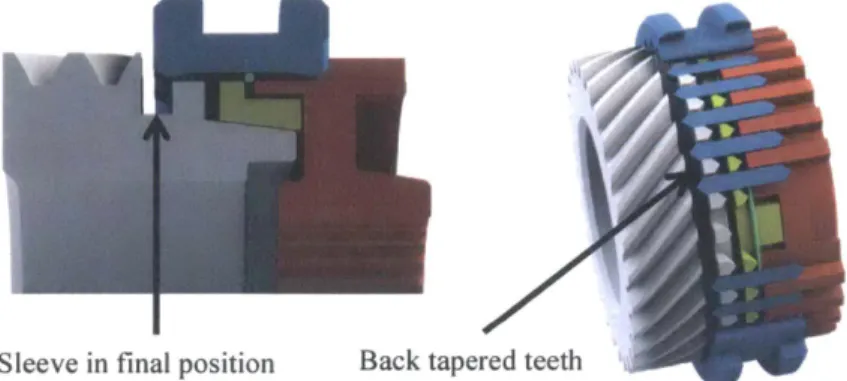
and gear dog teeth now aligned, the sleeve finally moves to its final, in-gear position. Its displacement is normally limited by a stop between the sleeve itself and the hub (see Figure 1-4). At this point, torque is transferred by the gear via the dog teeth to the sleeve and further via the hub to the output shaft [l]. To prevent decoupling under load, both dog teeth and sleeve splines are back tapered such that the torque between them also keeps them meshed [7]. Synchronization is concluded when the sleeve reaches its final position.

Sleeve in final position

Figure 1-10: Synchronization phase 6-Gear position assurance and torque transfer

The sleeve moves to its final position and is prevented from moving further by stops between

itself and the hub. Back tapers on the dog teeth and sleeve splines together with the transferred

torque maintain the sleeve in this meshed position.

1. 2. 3 Literature on mathematical model

In order to determine a synchronizer's braking capacity for a given vehicle and transmission, its equations of motion must be determined. Considering the entire vehicle dynamics as the system to be modeled is complex and requires models of many subsystems that are not available. Nevertheless, literature shows that simplifications can be made without risk of losing the important system characteristics. According to Paul D. Walker and N ong Zhang, if the synchronization time is small, and the inertia of the target gear is significantly smaller than that of the vehicle, it is possible to model the synchronizer as a rigid body with the inertia of the components to be synchronized reflected on that target gear [8]. This is the case in the clutchless transmission project. The inertia of the components of the synchronizer itself is negligible in comparison to the inertia of the system. Accordingly, in the simulations presented here these inertias are neglected, and the experiment introduced in Section 2 is designed to validate this assumption.

The synchronization process is described in 6 different stages, thus there is also the question of which are the significant sub-processes that should be taken into account to accurately describe the overall system behavior. However, the focus of this thesis is to characterize the

synchronizing potential and limitations of synchronizers in the configuration of the new

clutchless transmission. Then, the most important questions that this work aims to answer for a given synchronizer are the following: 1, whether the synchronizer, based on its geometry and material and the system's physical properties and starting conditions, can synchronize the speeds of the system and how fast it can do so; and 2, whether the material that makes up the synchronizer is strong enough to withstand the forces present during shifting in the new

transmission. The first question can be answered by looking into phases 2 and 3 of the synchronization process because the completion of these phases implies that the synchronizer is adequate. The experiment introduced in Section 2 addresses this. Section 6 addresses the second question.

Taking a look at phases 2 and 3 of the synchronization process, it is evident that what dominates the synchronization time is the action between cone surfaces that arises when an axial force is applied on the sleeve. Depending on the strength of the spring force of the detent mechanism, a fraction of the synchronization happens during phase 2. By varying the spring constant in simulations, A. P. Bedmar shows that a bigger portion of the synchronization is done in phase 2 with increasing spring constant, but with little change in total synchronization time [4]. Moreover the source of the synchronization torque is the same in phase 2 and phase 3, so without loss of generality, the synchronization can be assumed to occur solely in phase 3.

With the previous two assumptions, the most important torques in the system are the synchronization torque, the index torque, and the drag torque [8]. In addition, there is friction between the sliding fork and the rotating sleeve, which is expected to have a small effect compared to the cone torque. Then, the following differential equations describe the system:

Jhoh= -r -77f ₍₁₎

J hs ,-D,h

for the hub side, where Jh is the car inertia reflected on the hub side, (Oh is the angular velocity of

the hub, r, is the synchronization torque, TD,h is the drag torque of the engine reflected on the gear and Tf is the fork torque. And

Jcb = -T - TD,g ₍₂₎

for the gear side, where Jg is the engine inertia reflected on the gear, W2g is the angular velocity of

the gear, and TD,g is the drag torque of the engine reflected on the gear.

The synchronization torque is the central focus. The inertias, angular velocities, and drag torques are inputs that depend on the system to be synchronized, but the synchronization torque must be designed to meet the desired performance. According to A. P. Bedmar, it is a function of the axial force on the sleeve, the friction coefficients at the cone interface(s), and the geometry of the cones, and is given by

I c( -Rc I bL 2 2

rce = F(t)- (I+- - sin2 ac (3)

sin ac 3 Rc

where F is the fork force on the sleeve, pc is the coefficient of friction between cones, Re is the mean cone radius, ac is the cone angle measured from the shaft axis, and be is the half length of the cone generatrix [4]. This applies to a synchronizer with a single cone. The factor in parenthesis accounts for the change in radius across the surface of the cone, but it makes an insignificant difference and is neglected [5], [7]-[9]. If additional cones are present, each cone contributes with a torque given by the same expression as Eq. (3), but if multiple cones are

employed in the design, they are expected to have similar geometry and material properties. Then Eq. (3) can be rewritten as

T, = F (t) - )R (4)

sin ac

for the general case with Nc cones [7]. As for the angle ac, the smaller the value, the higher the torque it produces for a given force. But the constraint is that if it is too small, self-locking can occur as described in phase 4 of the synchronization. So the lower limit is

tan ac Mc ₍₅₎

to prevent self-locking [7].

The coefficient of friction between cone surfaces, p, is shown in Eq. (4) as a function of time

because it changes slightly at the beginning of phase 3 when the oil film has not yet been broken

and it is said to be in a mixed stage. This change in the value of the friction coefficient in the transition from hydrodynamic friction to solid friction is described by the Stribeck curve [4]. The simulation presented here neglects this edge effect because the mixed lubrication stage is assumed to last only a small fraction of the total synchronization time. Besides, all synchronizer rings are manufactured with grooves on the inside that are designed to break the oil film as fast as possible [9].

It has already been mentioned in the description of phase 3 that the synchronization torque must always be larger than the index torque, r1, while there is relative rotation of the gear with respect

to the hub. This blocking safety condition is met by designing the flank angles of the teeth

accordingly, such that ri< T, [10] where rj is given by

Fr RS 1-p tan( ' tan,/+,

where R, is the mean radius of the sleeve at the point of contact with the fork, ps is the coefficient of friction of the sleeve teeth, and f3 is the flank angle of the sleeve teeth. If the blocking safety is not met, clash between the sleeve splines and the gear dog teeth can occur [4], [7]. If it was not for this requirement, the flank angle fl could be designed smaller and that would make self-locking less of a problem because the same index torque is used for unlocking the ring from the gear cone in phase 4. In addition, the index torque must be larger than the drag on the gear during phase 5 to ensure that the drag does not take over once the friction ring is inactive [4]. The following condition must therefore be met.

r > TD,g ₍₇₎

Tf = pfFfR, (8)

where pf is the coefficient of friction between fork and sleeve. Lastly, the drag torques in Eqs. (1) and (2) are the reflected drag effects of the car and the engine on the hub and the gear respectively. Modeling drag torque precisely is complex as it has a high level of uncertainty and variability [8], but for the engine it can be approximated as being Coulombic [11] with the linear term proportional to the speed [4], [7], and for the hub side it can be estimated from the car drag (see Section 5.1).

2 Design of Experiment Setup 2.1 Purpose

Measuring a synchronizer's performance directly in the exact context in which it operates is complicated due to the complexity and inaccessibility of a vehicle transmission. Many aspects of a transmission that significantly affect the synchronization process such as vehicle and engine inertias, the drag generated by friction, thermodynamic effects [6], surface degradation [12] and vibration in the system are hard to model precisely. Nevertheless, the understanding of the basic mechanisms that dominate the behavior of the system as presented above permits to make approximations that can yield good estimates of the performance. The following experiment is designed to approximate the expected operating conditions of synchronizers in the clutchless transmission and monitor their performance given a set of known inputs. The results will make it possible to verify whether the analytical model of the system and the assumptions made above are valid for the clutchless transmission and to what extent.

2.2 Experiment requirements

The synchronizer is the object of the experiment, of course. The setup must allow for testing synchronizers of different sizes to ensure the results are generalizable. In addition, since lubrication is an important factor in the synchronization process, it must be included in the experiment. In order to emulate the engine inertia a flywheel with a large inertia is necessary. The flywheel represents the reflected inertia of the engine on the gear being synchronized. Also, it is important to model the drag of the engine, which is large. So the experiment should include a drag component. An axial force actuation mechanism is required for applying the input force on the sleeve fork while at the same time measuring this input force. The other two sensors needed are a tachometer for measuring the speed of the rotating components at all times and a timer for synchronizing the measurements and recording the time dependency of the process. The input variables to the system are the geometry and material properties of the synchronizer, the initial speed difference to be synchronized, the axial force exerted on the sleeve fork over time, and the inertia and drag of rotating components. The output is the synchronization time. Different values of the input variables need to be tested for the most reliable outcome.

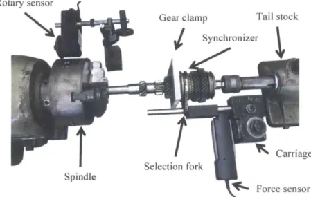
The experiment setup chosen is a manual lathe and is shown in Figure 2-1. The dynamic properties of a lathe fit the requirements that the experiment should implement a large inertia and include a drag component. Its versatility allows for mounting different sizes of synchronizers and shafts. The adjustability of the carriage makes it ideal for mounting different sleeve forks to provide the axial force for the different synchronizer sizes. Moreover, the ability of a lathe to change gear ratios between motor and spindle, provides a way of varying the inertia and drag of the system.

Rotary sensor

Gear clamp Tail stock

Selection fork Spindle

Figure 2-1: Lathe experiment setup for synchronizer engagement

The output shaft from a transmission is mounted between the spindle and the tail stock of a Monarch manual lathe. A custom clamp is used for restricting the rotation of the gear to be synchronized. The selection fork is mounted on the carriage such that the axial force can be measured with a force sensor. A rotary motion sensor measures the speed of the spindle.

The experiment is designed to obtain experimental data on synchronizers' braking performance

to compare to and verify the mathematical model. It is executed by starting the spindle with an

initial speed and then applying a known axial force to the sleeve towards the clamped gear,

thereby bringing the speed of the spindle to zero. In general in a transmission, both the engine side of the synchronizer and the wheels side are rotating during synchronization. This will

continue to be the case in the clutchless transmission. However, it is expected that the engine

side of the synchronizer will have a relatively much smaller reflected inertia, meaning that the wheels side is not expected to noticeably change its speed. In fact, from the perspective of the

comfort of a person in the vehicle, a perceptible deceleration of the car during an upshift (or

acceleration during a downshift) is undesirable. So the approximation that one side of the

synchronizer does not change speed during synchronization is adequate.

The fixed gear is a special case of a constant speed gear, but the speed difference between the

two sides is the variable of interest. Hence, the experiment is representative of all the cases in which one side of the synchronizer has an approximately constant speed during synchronization.

The only variable whose effect is different in the case of one side with a fixed, zero velocity with

respect to the case of one side with a fixed, nonzero velocity is the drag torque. The drag torque,

which is modeled as linear with velocity, has a larger impact at higher speeds. Nonetheless, the

and therefore it has a significant effect on the synchronization experiment. It is expected, then, that the model validity extends to the more general case of two spinning sides.

Multiple experiments were performed under different configurations in the following steps: The gears and synchronizers are assembled onto their corresponding shaft in the transmission. The shaft is mounted in the spindle on one end and supported by a revolving tailstock spindle on the opposite end. For each different synchronizer tested, an aluminum clamp was fabricated to fix the rotation of the related gear. To prevent the clamp from over-constraining the shaft, it restricts the rotation only by means of an extension rod that rests against the lathe bed (not visible in Figure 2-1). The selection fork is mounted on the tool post via a loosely fitted sleeve on a tool holder such that the motion parallel to the shaft is unrestricted. This allows the force sensor to be placed between the carriage and the synchronizer sleeve so that the input force is transmitted through it. A rotary sensor is placed behind the spindle and making contact with it to measure its angular velocity. Both sensors are connected to a computer through a LabPro data collection interface.

Each experiment run consisted of first starting the spindle with some initial speed and second applying an axial force on the selection fork using the lathe carriage to engage the synchronizer until the spindle speed decreased to zero. The data acquisition was triggered by the sudden increase in the applied force. Two synchronizers of different sizes were tested, and for each one the inertia and drag of the lathe were varied from a minimum, with the spindle disengaged from the gearbox, to a maximum, with the gearbox engaged. Multiple runs were executed for each unique configuration to ensure repeatability. Additionally, a few runs were executed without adding oil to the synchronizer to investigate the extent of the influence of lubrication. In the cases with the gearbox engaged, the electric motor was used to give the initial speed difference and in the case of the gearbox disengaged, the spindle was started manually.

3 Parameter Determination 3.1 Experiment parameters

In order to evaluate the model speed vs. time curves for the same inputs as the experimental curves, all the input parameters in Eqs. (1), (2), and (4) must be determined first. These parameters are not always available and in some cases it is not possible to measure them directly. While the synchronizer geometry (Re, be, ac, and

fi)

where Jpdl is the spindle inertia, cosad is the spindle angular velocity, r, is the manually induced

torque, Ddl/ is the rotational drag coefficient of the spindle, and -r,,, is the Coulombic drag torque of the spindle. Equation (9) is equivalent to Eqs. (1) and (2) except that in this case there is no synchronization torque. The drag torque is broken down into a linear component Dspdl-Owspd,

and a Coulombic (static) component Tc,spdl. Therefore, there are three parameters that need to be found in order to model the system correctly. Those are the spindle inertia Js dI, the linear drag

coefficient Dspd/, and the Coulombic friction Tespdl.

4

Figure 3-1: Experiment setup for parameter identification

(a) Setup for parameter determination experiment. A known torque input is applied to the lathe spindle using a force sensor and a string wound several turns around it. A rotary motion sensor measures the spindle speed over time. (b) Experimental data for spindle parameter determination.

Input torque (top) and speed response (bottom).

A simulator was created in Matlab (see Appendix A) to solve the above differential equation for

the same input torque vector of the experiment to find the three desired parameters that minimize the mean squared error with respect to the experimental response (effectively "fitting" the model to the experimental data). Figure 3-2 shows the resulting fit and parameters for the same data as Figure 3-1 (b), which corresponds to the spindle disconnected from the gearbox.

25 - _Experimental SimuLated 20 -J = 0.0427kg m2 - 5 - D,, =0.026kg -m2 ls 7d 1 T ,0. 177N - m S 10 -0 0.5 I 1.5 2 2.5 3 Time Is|

Figure 3-2: Simulated response of the spindle with optimized parameters

The experimental data is shown for the response of the spindle, disengaged from the gearbox, to a known, variable input torque. The speed increases up to about Is when torque is present and then decreases due to drag. The values found for inertia, drag coefficient, and Coulombic torque are shown. The mean squared error for this fit is 1.5134.

For each configuration tested, multiple runs were executed and the parameters were found in the

same manner. The results are given in Table 1 with 95% confidence interval.

Table 1-Dynamic parameters for configurations used in experiment

Parameter J,,, (kg -m2

) D,,11 (kg m2 / s) 7 ,, (N - m) Gearbox disengaged 0.0429 0.0002 0.026 0.002 0.18 0.01

(low inertia and drag) I I

Gearbox engaged 0.0895 0.0184 0.220 0.003 2.07 0.06

(high inertia and drag)

4 Evaluation of Experiment

Using the parameters found above and the model introduced in Section 1.2.3, a Matlab simulation was prepared (see Appendix B) for each of the different configurations of the experiment. The simulation was then compared to the experimental data to verify that the model is in agreement with the physical system and can be used to estimate synchronizer performance in a vehicle. Table 2 shows the relevant specifications of the synchronizers used in the experiments. The geometrical parameters where measured directly and the coefficients of friction

were taken from [9] for the cones and from [14] for the sleeve.

Table 2-Description of synchronizers used in experiment

Mean cone Cone COF Number Mean sleeve COF

diam. (mm) angle (0) cone (-) Cone material of cones diam. (mm) sleeve

Synchro. #1 49.1 6.7 0.13 brassalloy 1 71.0 0.12

4.1 Simulation results

Figure 4-1 shows the simulation result from an experiment for the lathe configuration with the smaller inertia and with synchronizer #1; Figure 4-2 for the same lathe configuration but with synchronizer #2; Figure 4-3 for the larger inertia configuration and with synchronizer #1; and Figure 4-4 for the larger inertia configuration with synchronizer #2.

---2(0 r 10 0 Simulated synchronized Experimental synchronized - Experimental unsynchronized 0.2 0.4 0.6 0.8 1 1.2 1.4 1.6 1.8 Time Isl Applied Force 0.2 0.4 0.6 0.8 Time 1.2 1.4 1.6 1.8 Isi

Figure 4-1: Small inertia experiment with synchronizer #1

(Top) The angular velocity of the spindle is plotted with respect to time for the unsynchronized and synchronized experimental data as well as for the simulated synchronization event. The unsynchronized data corresponds to the spindle slowing down due to its own drag. (Bottom) The corresponding input axial force on the fork is plotted.

0

300

r

200

-100 0

0 Simulated synchronized Experimental synchronized Experimental unsynchronized 2011 5 00 40 -4700 -~ 0 200 -0 1 1.2 1.4 1.6 1.8 Applied Force 0.6 0.8 1 1.2 1.4 1.6 1.8 Time Isl

Figure 4-2: Small inertia experiment with synchronizer #2

(Top) The angular velocity of the spindle is plotted with respect to time for the unsynchronized and synchronized experimental data as well as for the simulated synchronization event. (Bottom) The corresponding input axial force on the fork is plotted.

20 Ct 10 lo or 0 200 - 0 0-0

-K

(Top) The angular velocity of the spindle is plotted with respect to time for the unsynchronized and synchronized experimental data as well as for the simulated synchronization event. (Bottom) The corresponding input axial force on the fork is plotted.

I

30 2 20 S10 0 1 < 0 400 -Z 0 Simulated synchronized Experimental synchronized Experimental unsynchronized 0.1 0.2 0.3 0.4 0.5 0.6 0.7 Time Is| Applied Force 0 0.1 0.2 0.3 0.4 0.5 0.6 0.7 Time Isl

Figure 4-4: Large inertia experiment with synchronizer #2

(Top) The angular velocity of the spindle is plotted with respect to time for the unsynchronized and synchronized experimental data as well as for the simulated synchronization event. (Bottom) The corresponding input axial force on the fork is plotted.

4.2 Observations

These are some representative experiments of the 24 performed, all with similar results. Although every run is unique because the source of the force is manual (through the lathe carriage), these results show all the different configurations tested.

The diameter of the friction cone significantly affects the braking performance, in agreement with [4]. Comparing Figure 4-1 and Figure 4-2, it is evident that for a similar starting speed difference the synchronizer with the smaller diameter requires a substantially larger force to achieve a similar synchronization time.

The effect of the fork torque, which has been taken into account above, is small but not negligible. For example, not accounting for this torque in the case of a large inertia experiment with synchronizer #2 (Figure 4-4) results in an overestimation of the synchronization time by an extra 5%. _{This may or may not be significant depending on the desired accuracy. In this case,}

however, the synchronizers tested use only one friction cone, so the fork torque is expected to be less important in synchronizers with multiple cones.

Overall, the synchronization time tends to be slightly overestimated in the simulation with respect to the experimental data by up to about 7% (Figure 4-3). This may be a direct result of

the uncertainty of the coefficient of friction of the cone surfaces and the fact that it is assumed to

be constant in the simulation. Nevertheless, the results show that the proposed model does in fact describe well the most important characteristics of the synchronizing process. The model can

therefore be used to predict the performance of similar synchronizers in any transmission provided that the input parameters presented here are known.

5 Application in the Clutchless Transmission

In this section, the model validated above is used to estimate the performance of the available synchronizer in different possible scenarios in the clutchless transmission. The objective is to specify the relevant information needed for selecting and incorporating synchronizers in the new transmission. Normal operating conditions are assumed. Section 6 then gives an analysis of the possible extraordinaire conditions that may result in failure.

5.1 Parameters 5.1.1 Vehicle

In order to make predictions on synchronizer performance in a given transmission, the vehicle parameters must first be identified. The vehicle parameters of interest for a given upshift or downshift are the car and engine inertias and drags as reflected on the hub and the gear sides of the synchromesh. These principal parameters are represented in Figure 5-1.

Engine Transmission Differential Wheels

Synchromesh Gear

Figure 5-1: Schematic of the main inertial components

The most important parameters for the vehicle are the inertia of the engine, the inertia of the car as a whole, and their drags all reflected through gear ratios on the synchromesh. The inertia and drag of the engine (in red) is reflected on the gears depending on the gear ratio between them. The inertia and drag of the car and wheels (in green) is reflected on the shaft, and hence on the hub, through the differential.

The car inertia can be approximated from the mass of the car and the gear ratio between the

output shaft and the wheels. So the reflected inertia from the car on the hub J is given [15] by

R

M, = m, (10)

where the ratio in parenthesis is the apparent radius of the wheels at the output shaft of the transmission, mar is the mass of the car, R,, is the wheels radius, and r.,, is the final drive ratio between transmission output and wheels. The car drag accounts for the rolling resistance of the tires and the air drag. For the rolling resistance FD,,.r, the tires are approximated as equal and supporting an equal portion of the car's weight. It is given by the following equation [16]:

F = C,r(V>, mg (11)

1000

where C,.r is the rolling resistance coefficient of the tires and g is the gravitational acceleration. The rolling resistance coefficient Crr is a function of the speed of the vehicle vcar. From the data provided by the car manufacturer it can be described as linear as shown in Figure 5-2. The car tires are approximated to be all the same size and to contribute an equal amount of resistance.

15 Ofj

~1) Cr 14-t' 6

0 Data from car manufacturer

Linear best fit

0 20 40 60 80 100

Car speed I m/s I Figure 5-2: Rolling resistance of vehicle versus speed

The rolling resistance coefficient for the car is calculated for several speeds by averaging the front and rear wheel values provided by the car manufacturer. A linear to the data is made in order to make the calculations simpler.

The air drag coefficient C, as well as the frontal area Acar are provided by the car manufacturer. And the air drag, F),, is given by the following equation [17]:

F 7 -CIpAv4 V VZ11/ (12)

where Acar is the frontal area of the car and Vcar is the car speed. Combining Eqs. (11) and (12) and using the same apparent ratio in Eq. (10), the total reflected car drag on the synchronizer hub is

7 =

[ICpUA

A

which simplifies to 1 R3 4

s )('

(g

_m

The engine inertia is provided by the car manufacturer. And the reflected inertia on the gear, Jg depends on the gear ratio selected. The following simulations are calculated for shifts between ₁

st

J = rF,- JE (15)

where JE is the engine inertia. The engine drag is not provided and is difficult to measure. For the predictions in this section, it was estimated from [18] where the friction power of a 4-cylinder engine is determined. It is assumed that the engine friction is proportional to the number of cylinders, so the calculated drag coefficient from the 4-cylinder engine is scaled up to the 8-cylinder engine of the vehicle in question. Reference [18] does not directly calculate a drag coefficient of the engine but instead they give the friction power at different engine angular velocities. The drag coefficient is calculated under the assumption that the friction power is the product of the average friction torque over the piston cycle and the angular velocity of the engine. It is also noted from [18] that the friction power can be approximated as linear with respect to engine speed, with a constant Coulombic component and a linear one. The vehicle parameters used in the predictions are then given in Table 3.

Table 3-Vehicle parameters used for synchronizer performance predictions

Parameter Value

Car reflected inertia Jh=7.2028 [kg. m2]

Car reflected drag Ir, =0.000137[kg -m]$ +0.01045[kg . m2 /s] o +9.5982[N -m] Engine reflected inertia Jg =0.1052[kgm2] r,

Engine reflected drag T D,g = 0.1526[N -m -s] rETg + 35.0141[N -_{m] rET}

Before going into synchronization simulations, the engine behavior without any torque input other than its own drag is presented as a reference. Assuming that the engine starts at a speed co and is allowed to slow down by itself, using the estimated parameters in Table 3 the following is the expression for its speed over time.

O(t) = -229.45 - + w0 -229.45[ - e 1)38s (16)