A split Hopkinson pressure bar device to carry out confined friction tests under high pressures

HAL Id: hal-01564488

https://hal.archives-ouvertes.fr/hal-01564488

HAL is a multi-disciplinary open access archive for the deposit and dissemination of sci-entific research documents, whether they are pub-lished or not. The documents may come from

L’archive ouverte pluridisciplinaire HAL, est destinée au dépôt et à la diffusion de documents scientifiques de niveau recherche, publiés ou non, émanant des établissements d’enseignement et de

A split Hopkinson pressure bar device to carry out

confined friction tests under high pressures

Bastien Durand, Franck Delvare, Patrice Bailly, Didier Picart

To cite this version:

Bastien Durand, Franck Delvare, Patrice Bailly, Didier Picart. A split Hopkinson pressure bar device to carry out confined friction tests under high pressures. International Journal of Impact Engineering, Elsevier, 2016, 88, pp.54 - 60. �10.1016/j.ijimpeng.2015.09.002�. �hal-01564488�

A SPLIT HOPKINSON PRESSURE BAR DEVICE TO CARRY OUT CONFINED

1

FRICTION TESTS UNDER HIGH PRESSURES

2 3

Bastien Durand1_{, Franck Delvare}2_{, Patrice Bailly}3 _{and Didier Picart}4

4 5

1_{LMT, ENS-Cachan, 94235 CACHAN Cedex, France, bastien.durand@lmt.ens-cachan.fr,}

6

+33147402193 7

2_{Université de Caen, Normandie, Laboratoire N. Oresme, F-14032 Caen, France}

8

3_{INSA CVL, Laboratoire PRISME, F-18020 Bourges, France}

9

4_{CEA, DAM, Le Ripault, F-37260 Monts, France}

10 11

Abstract: Numerical simulations of mechanical loadings on pyrotechnic structures

12

require the determination of the friction coefficient between steel and explosives. Our study 13

focuses on contact pressures of around 100 MPa and sliding velocities of around 10 m/s. 14

Explosives are brittle materials which fracture when submitted to such pressures in uniaxial 15

compression. They have therefore to be confined to avoid any fracture during the tests. A new 16

Hopkinson bar device which simultaneously enables to confine a sample and rub it on steel 17

has therefore been designed. This device is composed of two coaxial transmission bars. It 18

consists in a cylindrical sample confined in a steel tube, the cylindrical sample being inserted 19

between the incident bar and the internal transmission bar, and the confinement tube being 20

leant against the external transmission bar. The high impedance of the external transmission 21

bar keeps the confinement tube quasi-motionless whereas the impedance of the internal 22

transmission bar is calculated to reach the desired pressure and the desired velocity at the 23

tube-sample interface. Tests have been carried out with an inert material mechanically 24

interface are deduced from strain measurements on the Hopkinson bars and on the external 26

face of the confinement tube, and from an analytical model. 27

28

Keywords: friction parameter, identification, confinement, split Hopkinson pressure bars

29 30

1 Introduction

31 32

Numerical simulations are performed to predict the ignition of confined explosives 33

submitted to accidental impacts [1], [2], [3]. Such impacts are characterised by velocities of 34

several tens of meters per second and are usually called “low-velocity impacts”. These 35

simulations are based on: 36

- An elasto-plastic model simulating the macroscopic behaviour, whose parameters are 37

identified from triaxial tests. 38

- A thermo-chemical model enabling the calculation of the local heat due to the irreversible 39

macroscopic strain and due to chemical reactions. 40

The parameters of the thermo-chemical model are identified from normalised experimental 41

tests supposed to reproduce accidental situations: the drop-weight test [4], the Steven-test [3], 42

[5], [6], the Susan-test [3] and the Taylor test [7] among others. Unfortunately, numerical 43

simulations of these normalised tests show that the ignition time of the explosive strongly 44

depends on the friction coefficient at the interface between the explosive and the contact 45

materials (generally steel). A test enabling the friction coefficient measurement between steel 46

and explosives under the “low-velocity impacts” conditions has therefore to be designed. 47

48

Numerical simulations display that the “low-velocity impacts” lead to contact 49

tribometers satisfy these requirements: tribometer with explosively-driven friction [8], target-51

projectile assembly with oblique impact [9], Hopkinson torsion bars [10], dynamometrical 52

ring with parallelepipedic specimen launched by a gas gun or an hydraulic machine [11] and 53

the friction of a pin on a revolving disc [12], [13]. With these classical tribometers, mainly 54

used on metals and ceramics, the friction samples are tested in simple compression and this 55

configuration is unfortunately not adapted to our situation, as explained above. 56

57

For safety reasons, our friction tests are carried out with an inert material mechanically 58

representative of an explosive. This material is named the I1. The I1 Young’s modulus is 59

2 GPa, its Poisson’s ratio  is estimated to 0.4 and its density is 1850 kg/m3 _{[14]. Its inelastic}

60

behavior has been studied by carrying out triaxial compression tests [14]. The material flow 61

when its plasticity threshold has been attained (for the sake of simplicity the maximal stresses 62

obtained using triaxial tests are used to define a plasticity threshold). The plasticity flow 63

threshold is defined by a Drucker-Prager criterion [14]: 64

65

(1) mis - P < C

66

where P is the hydrostatic pressure and mis the Von Mises equivalent stress.

67 68

Conventionally, the stress in the I1 is positive in compression and negative in traction. 69

A plastic incompressibility and a perfectly plastic behavior (i.e. C constant) are assumed. The 70

parameters have been determined: C = 25 MPa and α = 0.64 [14]. 71

72

According to relation (1), in the case of a simple compression loading, the maximum 73

axial stress is only 31 MPa. The I1 behavior is quasi-brittle, so when this limit stress is 74

tribometers because of the I1 fracture. The material has therefore to be confined during our 76

tests for two following reasons: 77

- The behavior of the confined material remains elastic even under high stresses. 78

- A confinement situation avoids any fracture to occur when the elasticity limit is reached. 79

A cylindrical I1 sample is thus enclosed in a steel tube. This technique is usually employed to 80

perform compression tests with quasi-uniaxial strain states [14], [15]. Our test bench has to be 81

designed to enables friction to occur between the I1 sample and the steel tube. Our 82

experimental configuration is similar to the compaction tests one [16], [17], [18]. 83

84

The Hopkinson bar set-up, its potential performances and the friction identification 85

from a test and from an analytical model are described in section 2. Then, the consistency of 86

this identification is verified in section 3 by performing numerical finite element simulations. 87

88

2 The Hopkinson bar set-up

89 90

2.1 Design and modeling 91

92

The Hopkinson bar device used for our friction tests has two coaxial output bars 93

(Figure 1). It consists in an I1 cylindrical sample confined in a steel tube, the sample being 94

inserted between the incident bar (via a plug, see Figure 2) and the internal output bar, and the 95

confinement tube being leant against the external output bar. The high impedance of the 96

external output bar keeps the confinement tube quasi-motionless whereas the impedance of 97

the internal output bar is calculated to reach the desired pressure and the desired velocity at 98

the tube-sample interface. Thus, the steel tube acts both as a confinement, which avoids any 99

fracture in the I1 sample, and as a friction surface. The radial pressure at the confinement 100

tube – sample interface is generated by the axial compression of the sample. 101

102

103

Figure 1: The Split Hopkinson Pressure Bar device. i: incident strain wave, r: reflected

104

strain wave, tu: strain measured on the confinement tube, et: external transmitted strain

105

wave, it: internal transmitted strain wave.

106 107

bar material Young’s modulus waves celerity diameters length external internal striker steel Ei = 166 GPa Ci = 4555 m/s 2Ri = 20 mm 1.05 m input 2.5 m internal output aluminum Eio = 72.8 GPa Cio = 5092 m/s 2Rio = 10 mm 1.46 m external output

steel Eeo = 205 GPa Ceo = 5162 m/s 2Reeo = 40 mm 2Rieo = 30 mm 1.5 m

Table 1: Young’s moduli, tensile/compressive waves celerities, diameters and lengths of the 108

bars. 109

110

The impact of the striker induces an incident compressive strain wave i in the input

111

bar (Figure 1). Reverberation occurs in the cell (cell details are given on Figure 2), which 112

leads to a reflected strain wave r in the input bar, to a transmitted compressive strain wave it

113

in the internal output bar and to a transmitted compressive strain wave et in the external

114

output bar. i and r are both measured by a longitudinal strain gauge glued on the input bar,

115

at 1.22 m from the plug interface, where the two waves are separated in time. it is measured

116

by a longitudinal strain gauge glued at 330 mm from the sample interface and et is measured

117

by a longitudinal strain gauge glued on the external face of the external output bar and at 118

295 mm from the confinement tube interface. 119

121

Figure 2 : Zoom on the mounting with the cell composed of the plug, the sample and the 122

confinement tube (axisymmetric cut view). 123

124

The sample has a diameter 2R and a length L equal to 10 mm, the confinement tube 125

has an external diameter 2Rt equal to 24 mm and the length scale is respected on Figure 2.

126

The confinement tube and the plug, made of steel, have a Young’s modulus Et and a Poisson’s

127

ratio t respectively equal to 200 GPa and to 0.29. The friction face of the confinement tube

128

has been reamed and the sample was turned on a sliding lathe. Both have a weak surface 129

roughness representative of the pyrotechnic structures roughness (arithmetic average of 130

absolute values Ra roughly equal to 0.8). The radial clearance between the plug and the tube

131

and between the internal output bar and the tube is of the order of 0.01 mm. Teflon sheets 132

have been inserted between the plug and the sample and between the internal output bar and 133

the sample in order to reduce the friction at these interfaces and thus increase the pressure at 134

the tube-sample interface. The circumferential gauge glued on the confinement tube is 2 mm 135

wide. The initial axial distance between the sample middle and the gauge middle is chosen 136

equal to 2.5 mm because the sample displacement relatively to the tube during the test is 137

supposed to be around 5 mm. Thus, the gauge is glued at the mean axial position of the 138

sample middle. 139

The force Fi applied by the input bar on the plug and the velocity Vi at the input bar -

141

plug interface can be determined from the Hopkinson formulae (2) and from strain waves i

142

and r measured by the gauge and virtually transported at the input bar - plug interface (see

143

Table 1 for symbols definitions): 144 145 (2)









The force Fio applied by the internal output bar on the sample and the velocity Vio at

148

the internal output bar - sample interface can be determined from the Hopkinson formulae (3) 149

and from strain wave it measured by the gauge and virtually transported at the internal output

150

bar - sample interface: 151 152 (3)         it io io it io io io C V E R F    2 153 154

The force Feo applied by the external output bar on the confinement tube and the

155

velocity Veo at the external output bar – confinement tube interface can be determined from

156

the Hopkinson formulae (4) and from strain wave et measured by the gauge and virtually

157

transported at the external output bar – confinement tube interface: 158 159 (4)





The equilibrium state of the cell (i.e. the confinement tube, the sample and the plug) 162 gives: 163 164 (5) Fi = Feo+Fio 165 166

The stationary state of the cell gives: 167

168

(6) Vi = Vio

169 170

In the case of a stationary state, the sliding velocity at the friction interface V can be 171 expressed as following: 172 173 (7) V = Vio - Veo or V = Vi - Veo 174 175

The sample behavior has to be modeled to obtain a second relation between the forces 176

Fi, Feo and Fio. The model used is similar of the Janssen’s one [19] and has been previously

177

used by the authors in [20] and [21]. The approach is based on three assumptions: 178

(i) the confinement tube is assumed to be perfectly rigid, 179

(ii) the sample behavior remains elastic, 180

(iii) in the sample, the axial, radial and circumferential stresses and strains do not depend on 181

the radial coordinate. 182

184

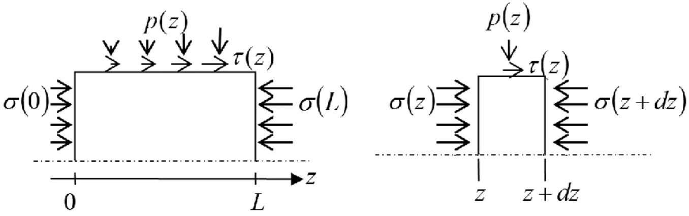
Figure 3: Stresses in the sample. z: axial coordinate, p(z): radial pressure, (z): friction stress 185

applied by the tube on the interface, (z): axial stress. 186

187

If the stresses in the sample (Figure 3) are positive in compression and negative in 188

traction, the Hooke’s law leads to the following relation: 189 190 (8)

 

_{ }

 being the I1 Poisson’s ratio. 192

193

The axial equilibrium of the sample slice between z and z+dz (Figure 3) leads to: 194 195 (9)

 

 

 

R being the sample radius.

197 198

A Coulomb’s law with a friction coefficient denoted f at the tube-sample interface 199

leads to: 200

203

The relations (8), (9) and (10) lead to a differential equation: 204 205 (11)

 

 





By taking into account the boundary conditions: 208 209 (12)

 

 





_

_

The incident strain wave i can be linked to the impact velocity of the striker Vs:

216 217 (14) i s i C V 2    218 219

Thanks to the Hopkinson formulae (2), (3) and (4), thanks to the equilibrium state 220

equation (5), thanks to the stationary state equation (6), and thanks to relation (13), the mean 221

pressure along the friction interface pmean and the sliding velocity V can be determined from

222

the impact velocity of the striker Vs, from the friction coefficient f and from the set-up

225 (15)













]

[

















Relations (15) and (16) enable to choose the apparatus dimensions (L, R, Ri, Rio, Reeo

230

and Rieo), the apparatus materials (Ei, Ci, Eio, Cio, Eeo and Ceo) and the striker initial velocity Vs

231

knowing the sample Poisson’s ratio , the friction coefficient f and the desired interface

232

solicitations (pmean and V). It must be highlighted that an accurate calculation of the apparatus

233

needs to know a priori an order of the friction coefficient f magnitude and needs to know 234

accurately the sample Poisson’s ratio . The striker of our apparatus can be launched at

235

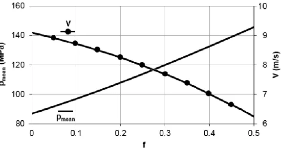
10 m/s. Figure 4 therefore displays the magnitudes of the mean pressure and of the sliding 236

velocity that can be reached with our set-up. Figure 4 shows that the mean pressure increases 237

and that the sliding velocity decreases when the friction coefficient increases. The desired 238

100 MPa pressure and the desired 10 m/s sliding velocity can almost be simultaneously 239

approached for very low friction coefficients (lower than 0.1). It could be noted that the 240

pressure and the sliding velocity cannot be simultaneously imposed to a desired value because 241

one depends on the other. 242

244

Figure 4 : Evolution of the mean pressure pmean and of the sliding velocity V as a function of

245

the friction coefficient f. 246

247

None of the former devices enables to reach such friction solicitations. The tribometer 248

used in [20] enables to reach a sliding velocity of around 10 m/s but limits the mean pressure 249

to 20 MPa whereas the tribometer used in [21] and in [22] enables to reach a mean pressure of 250

around 100 MPa but limits the sliding velocity to 2 m/s. 251

252

2.2 Analysis of measurements 253

254

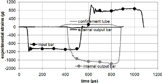
A test has been conducted to experimentally check if the sample reaches a stationary 255

equilibrium state as assumed in section 2.1. The time evolutions of the raw strains are shown 256

on Figure 5. The forces applied by the bars on the cell and the velocities at the bars-cell 257

interfaces are then determined from the Hopkinson formulae (2), (3) and (4). The input force 258

can be compared to the output force on Figure 6 and the sample input velocity can be 259

compared to the sample output velocity on Figure 7. 260

262

Figure 5: Time evolutions of the raw strains measured by the gauges glued on bars and on the 263

confinement tube. The strain measured on the external output bar is very low compared to the 264

others. 265

266

We can notice that the time beginning used on Figure 5 is different from the one used 267

on the other figures and will be no more used in the paper. 268

270

Figure 6: Time evolutions of the input force Fi and of the sum of the external output force and

271

of the internal output force Feo+Fio deduced from the measured strain waves in the bars and

272

from the Hopkinson formulae. 273

274

275

Figure 7: Time evolutions of the input velocity Vi, of the internal output velocity Vio and of

276

the external output velocity Veo deduced from the measured strain waves in the bars and from

277

the Hopkinson formulae. 278

A quite satisfactory stationary equilibrium state can be observed on Figure 6 and 280

Figure 7. The evolution of the experimental input force Fi during the transient phase (at the

281

beginning) can be explained by the time shifting of the incident and the reflected waves i and

282

r. These two waves being quasi-opposed (Figure 8), uncertainties are amplified when the

283

input force is calculated with formula (2). The experimental evolution of Fi will therefore not

284

be used to identify the friction coefficient f and we will focus only on the stationary phase 285

(approximately from 300 µs to 400 µs). 286

287

288

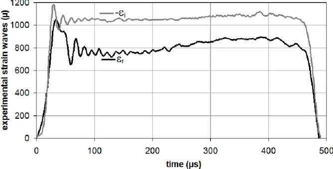
Figure 8: Time evolutions of the opposite of the measured incident strain wave i and of the

289

measured reflected wave r, both virtually transported at the input bar - plug interface.

290 291

Figure 7 shows that the sliding velocity V is of the order of 8-9 m/s during the 292

stationary phase. 293

According to relations (5) and (13), the friction coefficient f can be deduced from the 295

output forces ratio

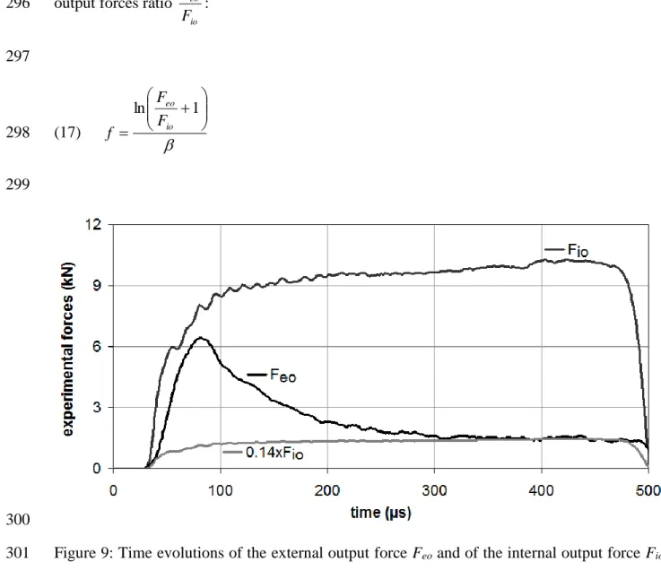
io eo F F : 296 297 (17)          1 ln io eo F F f 298 299 300

Figure 9: Time evolutions of the external output force Feo and of the internal output force Fio

301

deduced from the measured strain waves in the bars and from the Hopkinson formulae. 302 303 The io eo F F

ratio identified during the stationary phase on Figure 9 in roughly 0.14. By 304

using relation (17), it leads to  f  0.13 and if   0.4 to f  0.05. 305

306

The mean friction stress mean can be deduced from Feo which corresponds to the

309 (18) RL F_eo mean   2  310 311

The minimal pressure pmin is reached on z = 0 and the maximal pressure pmax in

312

reached on z = L (Figure 3). According to relations (5), (8) and (12), pmin and pmax can be

313

expressed from the output forces Feo and Fio:

314 315 (19)

 

 

According to relations (8), (9) and (10), the pressure p is an exponential function of 318 (f z): 319 320 (20)

_

_

For low magnitudes of f, p can thus be considered as an affine function of z, which 323 implies: 324 325 (21) 2 max min p p p_mean   326 327

The mean interface stresses are determined from the experimental output forces F 328

330

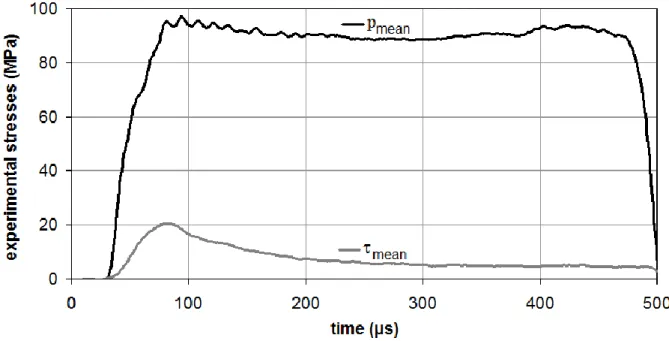
331

Figure 10: Time evolutions of the experimental mean pressure pmean and of the experimental

332

mean friction stress mean.

333 334

Figure 10 shows that the mean pressure pmean is of the order of 90-100 MPa.

335 336

3 Numerical simulations of the test: check of the results consistency

337 338

Finite element simulations (software: ABAQUS/Explicit) are performed in order to 339

check the consistency of the experimental results and of the friction coefficient magnitude 340

identified from our analytical model (f  0.05). The whole set-up except for the striker is 341

exactly reproduced in these simulations. As Teflon sheets have been inserted between the 342

plug and the sample and between the internal output bar and the sample, these contacts are 343

supposed to be frictionless. The experimental incident strain wave i is used as an imposed

344

loading by applying on the right-hand extremity of the input bar (Figure 1) a pressure equal to 345

input bar Young’s modulus Ei. The opposite of i can be seen on Figure 8. The strains r, tu,

347

et and it can be considered as the mechanical response of the set-up to i and the simulations

348

have been performed with several values of the friction coefficient f to study its influence on 349

the response. 350

351

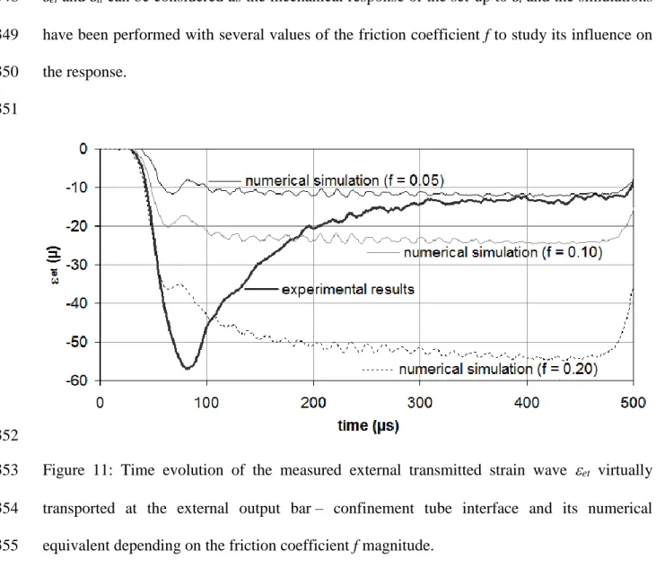
352

Figure 11: Time evolution of the measured external transmitted strain wave et virtually

353

transported at the external output bar – confinement tube interface and its numerical 354

equivalent depending on the friction coefficient f magnitude. 355

356

The numerical equivalent of the strain measured by the gauge glued on the 357

confinement tube tu is actually the mean value of the numerical circumferential strain along

358

the gauge width. 359

361

Figure 12: Time evolution of the strain measured by the gauge glued on the confinement tube 362

tu and its numerical equivalent depending on the friction coefficient f magnitude.

363 364

365

Figure 13: Time evolution of the measured reflected strain wave r virtually transported at the

366

input bar - plug interface and its numerical equivalent depending on the friction coefficient f 367

magnitude. 368

370

Figure 14: Time evolution of the measured internal transmitted strain wave it virtually

371

transported at the internal output bar - sample interface and its numerical equivalent 372

depending on the friction coefficient f magnitude. 373

374

The external transmitted strain wave et is proportional to the friction force and is

375

therefore the most friction dependent strain (Figure 11). During the stationary phase, f = 0.05 376

is a very good fit with the experimental et. The strain measured on the confinement tube tu is

377

also highly dependent on f, but a perfect fit cannot be obtained because of the numerical 378

strains high values (Figure 12). The reflected strain wave r and the internal transmitted strain

379

wave it are quasi-independent on friction (Figure 13 and Figure 14). During the stationary

380

phase, f = 0.05 is consistent with the measured r and with the measured it.

381 382

4 Discussion of the analytical model assumptions

383 384

Relation (17) leads to the following one: 385

(22)



 



387 388

389

Figure 15: Time evolutions of the numerical external output force Feo and of

390









392

Figure 15 shows that the analytical model slightly overestimates the friction force Feo.

393

Only this criterion finally matters because f is firstly identified from the

io eo F F ratio. 394 395 5 Conclusion 396 397

The purpose was to design a set-up enabling the friction measurement between an inert 398

material, mechanically representative of explosives, and a steel confinement. The desired 399

sliding velocities and the desired pressures were respectively 10 m/s and 100 MPa. A 400

confinement set-up using the split Hopkinson pressure bars technique had to be designed 401

compression of classical tribometers. Such a configuration does not enable to make direct 403

measurements. As a result, the stresses and the friction coefficient at the interface between 404

steel and the inert material were identified from indirect measurements, from an analytical 405

model and from the value of the inert material Poisson’s ratio. It has been shown that the 406

sliding velocity and the pressure reached roughly 8-9 m/s and 90-100 MPa whereas the striker 407

was launched at only 10 m/s. 408

409

A very low friction coefficient has been measured: only 0.05. In [20] and [21], a 410

sliding velocity of the order of 1 mm/min has been imposed and the corresponding friction 411

coefficient is roughly 0.2. In [22], the mean pressure is approximately 70 MPa and the sliding 412

velocity is of the order of 2 m/s. In [20], the mean pressure is approximately 20 MPa and the 413

sliding velocity is around 10 m/s. In both cases, the friction coefficient is of the order of 0.4-414

0.5. The reasons of such a variation should be studied in a future work. The friction drop at 415

the very beginning of the test could also be studied by using a time dependent friction model. 416

417

The measurements processing could also be improved by using an inverse method like 418

in [23]. Another prospect is the design of a compaction test enabling the friction force 419

measurement. Indeed, the study of the friction in compaction situations is an issue [16], [18] 420

and our device enables the simultaneous determination of the friction parameters and of the 421

compacted material parameters. 422

423

Acknowledgments: The authors would like to thank Maxime Biessy for his help and the

424

reviewers for their valuable comments. 425

6 References

427 428

[1]: Picart D, Delmaire-Sizes F, Gruau C, Trumel H. Ignition of a HMX-based PBX 429

submitted to impact: strain localisation and boundary condition. 16th _{Conference of the}

430

American Physical Society Topical Group on Shock Compression of Condensed Matter 431

(2009). 432

433

[2]: Picart D, Bouton E. Non-shock ignition of a HMX-based high explosive: thermo-434

mechanical numerical study. 14th _{International Detonation Symposium, Coeur d'Alène,}

435

USA (2010). 436

437

[3]: Picart D, Ermisse J, Biessy M, Bouton E, Trumel H. Modelling and simulation of 438

plastic-bonded explosive mechanical initiation. International Journal of Energetic 439

Materials and Chemical Propulsion, 12(6), 487-509 (2013). 440

441

[4]: Field JE, Swallowe GM, Heaven SN. Ignition mechanisms of explosives during 442

mechanical deformations. Proceeding of the Royal Society London A, 383, 231-44 443

(1982). 444

445

[5]: Gruau C, Picart D, Belmas R, Bouton E, Delmaire-Sizes F, Sabatier J, Trumel H. 446

Ignition of a confined high explosive under low velocity impact. International Journal of 447

Impact Engineering 36, 537–550 (2008). 448

[6]: Vandersall KS, Chidester SK, Forbes JW, Garcia F, Greenwood DW, Switzer LL and 450

al. Experimental and modelling studies of crush, puncture, and perforation scenarios in 451

the Steven impact test. Office Naval Research 333-05-02, (Eds.), Proceedings of the 452

12th _{International Detonation Symposium, San Diego, 131–139 (2002).}

453 454

[7]: Yodo A and al. Energetic materials for defense - Safety, vulnerability - Friability. 455

AFNOR NF EN 16701 (2014). 456

457

[8]: Kim HJ, Emge A, Winter RE, Keightley PT, Kim WK, Falk ML, Rigney DA. 458

Nanostructures generated by explosively driven friction: Experiments and molecular 459

dynamics simulations. Acta Materiala, 57(17), 5270-5282 (2009). 460

461

[9]: Rajagopalan S, Irfan MA, Prakash V. Novel experimental techniques for investigating 462

time resolved high speed friction. Wear, 225-229, Part 2, 1222-1237 (1999). 463

464

[10]: Huang H, Feng R. Dynamic Friction of SiC Surfaces: A Torsional Kolsky Bar 465

Tribometer Study. Tribology Letters, 27, 329-338 (2007). 466

467

[11]: Philippon S, Voyiadjis GZ, Faure L, Lodygowski A, Rusinek A, Chevrier P, Dossou E. 468

A Device Enhancement for the Dry Sliding Friction Coefficient Measurement Between 469

Steel 1080 and VascoMax with Respect to Surface Roughness Changes. Experimental 470

Mechanics, 51(3), 337-358 (2011). 471

[12]: Dickson PM, Parker GR, Smilowitz LB, Zucker JM, Asay BW. Frictional Heating and 473

Ignition of Energetic Materials. CP845, Conference of the American Physical Society 474

Topical Group on Shock Compression of Condensed Matter, 1057-1060 (2005). 475

476

[13]: Hoffman DM, Chandler JB. Aspect of the tribology of the plastic bonded explosive LX-477

04. Propellants, Explosives, Pyrotechnics 29, 368–373 (2004). 478

479

[14]: Bailly P, Delvare F, Vial J, Hanus JL, Biessy M, Picart D. Dynamic behavior of an 480

aggregate material at simultaneous high pressure and strain rate: SHPB triaxial tests. 481

International Journal of Impact Engineering, 38, 73-84 (2011). 482

483

[15]: Forquin P, Safa K, Gary G. Influence of free water on the quasi-static and dynamic of 484

strength of concrete in confined compression tests. Cement and Concrete Research, 40, 485

321-333 (2009). 486

487

[16]: Azhdar B, Stenberg B, Kari L. Determination of dynamic and sliding friction, and 488

observation of stick-slip phenomenon on compacted polymers during high velocity 489

compaction. Polymer Testing, 25, 1069–1080 (2006). 490

491

[17]: Burlion N, Pijaudier-Cabot G, Dahan N. Experimental analysis of compaction of 492

concrete and mortar. International Journal for Numerical and Analytical Methods in 493

Geomechanics, 25(15), 1467-1486 (2001). 494

[18]: Yong-Ming Tien, Po-Lin Wu, Wei-Hsing Huang, Ming-Feng Kuo, Chen-An Chu. Wall 496

Friction measurement and compaction characteristics of bentonite powders. Powder 497

Technology 173, 140-151 (2007). 498

499

[19]: Janssen HA. Versuche über Getreiedruch in Silozellen. Vereins Z Deutsch Eng 39, 1045 500

(1895). 501

502

[20]: Durand B, Delvare F, Bailly P, Picart D. Friction between steel and a confined inert 503

material representative of explosives under severe loadings. Experimental Mechanics 504

DOI 10.1007/s11340-014-9885-z (2014). 505

506

[21]: Durand B, Delvare F, Bailly P, Picart D. Identification of the friction under high 507

pressure between an aggregate material and steel: experimental and modelling aspects. 508

International Journal of Solids and Structures, 50(24), 4108-4117 (2013). 509

510

[22]: Durand B, Delvare F, Bailly P, Picart D. A friction test between steel and a brittle 511

material at high contact pressures and high sliding velocities. 10th International

512

DYMAT Conference (2012). 513

514

[23]: Durand B, Delvare F, Bailly P. Numerical solution of Cauchy problems in linear 515

elasticity in axisymmetric situations. International Journal of Solids and Structures, 21, 516

3041-3053 (2011). 517