Income and wealth concentration in Spain in a historical and fiscal perspective

HAL Id: halshs-00587714

https://halshs.archives-ouvertes.fr/halshs-00587714

Preprint submitted on 21 Apr 2011

HAL is a multi-disciplinary open access

archive for the deposit and dissemination of sci-entific research documents, whether they are pub-lished or not. The documents may come from teaching and research institutions in France or abroad, or from public or private research centers.

L’archive ouverte pluridisciplinaire HAL, est destinée au dépôt et à la diffusion de documents scientifiques de niveau recherche, publiés ou non, émanant des établissements d’enseignement et de recherche français ou étrangers, des laboratoires publics ou privés.

Facundo Alvaredo, Emmanuel Saez

To cite this version:

Facundo Alvaredo, Emmanuel Saez. Income and wealth concentration in Spain in a historical and fiscal perspective. 2007. �halshs-00587714�

WORKING PAPER N° 2007 - 39

Income and wealth concentration in Spain in a

historical and fiscal perspective

Facundo Alvaredo Emmanuel Saez

JEL Codes: D3, H2, N3, O1

Keywords: Income concentration, top incomes, behavioral response

P

-

S

E

L

’E

A

-

48,BD JOURDAN –E.N.S.–75014PARIS TÉL. :33(0)143136300 – FAX :33(0)143136310

www.pse.ens.fr

CENTRE NATIONAL DE LA RECHERCHE SCIENTIFIQUE –ÉCOLE DES HAUTES ÉTUDES EN SCIENCES SOCIALES

Income and Wealth Concentration in Spain in a

Historical and Fiscal Perspective

Facundo Alvaredo, Paris School of Economics and CREST Emmanuel Saez, UC Berkeley and NBER

Abstract

This paper presents series on top shares of income and wealth in Spain over

the 20th century using personal income and wealth tax return statistics. Top

income shares are highest in the 1930s, fall sharply during the first two decades of the Franco dictatorship, and have increased slightly since the 1960s, and especially since the mid-1990s. The top 0.01% income share in Spain estimated from income tax data is comparable to estimates for the United States and France over the period 1933-1971. Those findings, along with a careful analysis of all published tax statistics, suggest that income tax evasion and avoidance among top income earners in Spain before 1980 was much less prevalent than previously thought. Wealth concentration has been about stable from 1982 to 2004 as surging real estate prices have benefited the middle class and compensated for a slight increase in financial wealth concentration in the 1990s. We use our wealth series and a simple conceptual model to analyse the effects of the wealth tax exemption of stocks for owners-managers introduced in 1994. We show that the reform induced substantial shifting from the taxable to tax exempt status. This shifting has eroded the wealth tax base substantially and hence the tax exemption has generated large efficiency costs.

JEL Codes: D3, H2, N3, O1

Keywords: Income Concentration, top incomes, behavioral response

Facundo Alvaredo, PSE-ENS, 48 Boulevard Jourdan, 75014 Paris, France, alvaredo@pse.ens.fr, Emmanuel Saez, University of California at Berkeley, Department of Economics, 549 Evans Hall #3880, Berkeley, CA 94720, USA, saez@econ.berkeley.edu. We thank Tony Atkinson, Orazio Attanasio, Luis Ayala, Olympia Bover, Samuel Calonge, Juan Carluccio, Francisco Comín, Carlos Gradín, Jorge Onrubia, Cesar Perez, Thomas Piketty, Leandro Prados de la Escosura, Javier Ruiz-Castillo, Jesús Ruiz-Huerta, Mercedes Sastre, Rafael Vallejo Pousada, four anonymous referees, and many seminar participants at PSE, CREST (Paris), and IEF (Madrid) for helpful comments and discussions. Financial support from the Fundación Carolina (Facundo Alvaredo) and the Sloan Foundation and NSF Grant SES-0134946 (Emmanuel Saez) is thankfully acknowledged.

1. Introduction

The evolution of income and wealth inequality during the process of development has attracted enormous attention in the economics literature. A number of recent studies have constructed series for shares of income accruing to upper income groups for various countries using income tax statistics. Most of those studies are gathered in a volume edited by Atkinson and Piketty, 2007. The countries studied are Anglo-Saxon countries (United Kingdom, Ireland, United States, Canada, New Zealand and Australia) and continental European countries (Finland, France, Germany, Netherlands, Sweden, and Switzerland) and large Asian countries (China, India, Indonesia, and Japan). No such study has analyzed Southern European countries. This paper proposes to start filling this gap by analyzing the Spanish experience. Spain is an interesting country to analyze on several grounds.

First, there are very few studies on the evolution of inequality in Spain from a historical perspective. A number of studies have analyzed the evolution of income, earnings and expenditure inequality over the last three decades using survey data. Research has also been done using income tax data for

recent years.1 Survey-based studies point to a reduction in income or

expenditure inequality in the 1970s followed by relative stability in the 1980s and 1990s, while tax-based results display a worsening in the distribution of income in 1982-1991 and 1995-1998. Garde, Ruiz-Huerta, and Martínez,

1995, provide a survey of the literature until 1995.2 More recently, Prados de

la Escosura, 2006a, 2007b has constructed long historical series on income inequality such as ratios of GDP per capita to low skill wages or average wages, as well as industry wage differentials. Those estimates are not based

1 _{Those studies, which include Castañer, 1991, Lasheras et al., 1993, Ayala and Onrubia,} 2001, and Rodríguez and Salas, 2006, focus primarily on the redistributive power of the income tax. They estimate global inequality indices such as Gini before and after taxes and do not specifically focus on top income groups as we do here.

2 _{For key studies on income inequality in Spain over the last decades, see Alcaide, 1967,} 1974, 1999, Alcaide and Alcaide, 1974, 1977, 1983, Alvarez et al., 1996, Ayala and Onrubia, 2001, Ayala and Sastre, 2005, Ayala et al., 1993, Bosch et al., 1989, Budría and Díaz-Giménez, 2007, Cordero et al., 1988, Del Río and Ruiz-Castillo, 2001a,b, Escribano, 1990, Febrer and Mora, 2005, Goerlich and Mas, 2001, 2004, Gradín, 2000, 2002, Martín-Guzmán et al., 1996, Oliver I Alonso et al. 2001, Pascual and Sarabia, 2004, Ruiz-Castillo, 1987,

on micro-data but offer the best evidence to date on inequality trends in Spain from a historical perspective. Therefore, our study can be seen as the first serious attempt at compiling systematic and long run series of income concentration using primarily individual tax statistics, a source that has not been fully exploited by previous studies. It is also important to note that our series measure only top income (or wealth) concentration and hence are silent about changes in the lower and middle part of the distribution. As a result, our series can very well follow different patterns than broader measures of inequality such as Gini coefficients or macro-based estimates, an important point we will emphasize throughout.

Second, up to the 1950s, Spain was still largely an agricultural economy with a GDP per capita around $4,000 (in today dollars) similar to

developing countries such as Pakistan or Egypt today.3 Indeed, because of

the civil war shock and the poor economic performance during the first two decades of the Franco dictatorship, Spain GDP per capita did not reach the peak of 1929 before 1951. Starting in the 1950s and following economic liberalization and openness to trade, economic growth resumed at a very quick pace. Today, Spain’s GDP per capita is only about 20% lower than GDP per capita of the largest western European economies such as France, Germany, or the United Kingdom. Therefore, it is quite interesting to analyze income concentration during the stagnation years and during the economic boom starting in the late 1950s to re-assess the link between economic development and income concentration.

Third, Spain has undergone dramatic political changes since the 1930s. Spain was a republic from 1931 to 1939. A progressive government first ran the republic from 1931 to 1933, followed by a conservative government from 1933 to 1935, when some reforms of the previous years were abandoned. The reformist parties returned to power in 1935; however, the division between the advocates of the democratic changes and those

1998, Ruiz-Castillo and Sastre, 1999. A summary of the key findings can be found in the appendix.

3 _{Prados de la Escosura, 2003, 2006b, 2007a has constructed historical GDP and growth} series for Spain. He emphasizes that, before the economic stagnation of the 1930-1952 period, Spain experienced significant economic growth since 1850, in particular from 1850-1883 and in the 1920s. Maddison, 2001, 2003 also reproduces those historical series of real GDP per capita in Spain in his international compilation.

supporting a revolutionary process became evident soon. A military coup lead by General Franco, followed by a three year long civil war, transformed Spain into a dictatorship from 1939 till the death of Franco in 1975. Since then, Spain has returned to democracy and was run from 1982 to 1996 by the Socialist party, which tried to implement progressive policies such as the development of progressive income and wealth taxation, and of a welfare state with universal health coverage. The study of top income and wealth shares in Spain can cast light on the effects of the political regime and economic policies on inequality and concentration.

Finally, over the last twenty years, Spain has implemented large income and wealth tax reforms among which sharp reductions in top income marginal tax rates. Spain has also modified the wealth tax base by exempting corporate stocks and business assets for corporate and business owners actively involved in managing the business in 1994. Our constructed top income and wealth shares can be used to cast light on the effects of taxation on the economic and tax avoiding behavior of the affluent. We propose a detailed application in the case of the 1994 wealth tax exemption.

Our results show that income concentration was much higher during the 1930s than it is today. The top 0.01% income share estimated from reported incomes was about twice higher in the 1930s than over the last two decades. The top 0.01% income share fell sharply during the first two decades of the Franco dictatorship, and has increased slightly since the 1970s, and especially since the mid-1990s. Interestingly, both the level and the time pattern of the top 0.01% income share in Spain is fairly close to comparable estimates for the United States (Piketty and Saez, 2003) and France (Piketty, 2001, 2003) over the period 1933-1971, especially the post-World War II decades. Those findings, along with a careful analysis of all published tax statistics as well as a re-evaluation of previous academic work on income tax evasion in Spain, leads us to conclude that income tax evasion and avoidance in Spain before 1980 was much less prevalent than previously thought at the top of the distribution. As a result, those income tax statistics are a valuable primary data source for analysing income concentration.

Over the last two decades, top income shares have increased significantly due to an increase in top salaries and a surge in realized capital

gains. The gains, however, have been concentrated in the top percentile (and especially the top fractiles within the top percentile) with little changes in income shares of upper income groups below the top percentile. Financial wealth concentration has also increased in the 1990s due to a surge in stock prices, which are held disproportionately by the wealthy. However, real estate prices have increased sharply as well. As real estate wealth is less concentrated than financial wealth, on net, top wealth shares (including both financial and real estate wealth) have declined slightly during the period 1982-2002.

The data show that the wealth tax exemption of stocks for owner-managers since 1994 has gradually and substantially eroded the wealth tax base, especially at the very top: by 2002, the top 0.01% wealth holders could exempt about 40% of their wealth because of this exemption. We develop a simple conceptual model to explain this phenomenon, which we estimate using our wealth series. Our empirical results show evidence of very strong shifting effects whereby wealthy business owners were able to re-organize their business ownership and activities in order to take advantage of the reform. This suggests that this tax exemption both reduced the redistributive power of the progressive wealth tax and created substantial deadweight burden as business owners were taking costly steps to qualify for the exemption. The case study of the wealth tax exemption illustrates how our series can be used to cast light on the evaluation of tax policy reforms.

The paper is organized as follows. Section 2 describes our data sources, outlines our estimation methods, and discusses the issue of income tax evasion in Spain. In Section 3, we present and analyze the trends in top income shares since 1933 as well as the composition of top incomes since 1981. Section 4 focuses on top wealth shares and composition since 1982. Section 5 uses the wealth series to analyze the efficiency costs of the wealth tax exemption of 1994. Finally, Section 6 offers a brief conclusion. The complete details on our data and methods, as well as the complete sets of

results are presented in appendix.4

2. Data, Methodological Issues, and Context

2.1. Data and Series Construction

Our estimates are from personal income and wealth tax return statistics compiled by the Spanish fiscal administration for a number of years from 1933 to 1971 and annually from 1981 on. The statistical data presented are much more detailed for the 1981-2004 period than for the older period. Because the received wisdom is that the individual income tax was poorly enforced, especially in the pre-1981 period, we will discuss in great detail this issue in Section 2.2 and throughout the text in Section 3. Complete details on the methodology are provided in appendix.

Before 1981, because of very high exemption levels, only a very small fraction of individuals had to file individual tax returns and therefore, by necessity, we must restrict our analysis to the top 0.1% of the income distribution (and for 1933-1949 even the top 0.01%). From 1981 on, we can analyze the top 10% of the income distribution. Spain has adopted an annual personal wealth tax since 1978. Detailed statistics on the ‘new’ income and

wealth tax have started to be published in 1981 and 1982 respectively.5 The

progressive wealth tax has high exemption levels and only the top 2% or 3% wealthiest individuals file wealth tax returns. Thus, we limit our analysis of wealth concentration to the top 1% and above, and for the period 1982 to 2004. For 1981 to the present, estimates are based on Spain excluding two autonomous regions: Pais Vasco and Navarra, because they manage the income tax directly and hence are excluded from the statistics. Those two regions represent about 10% of Spain in terms of population and income. From 1933 to 1935, estimates are based on all Spain; Navarra is excluded since 1937 and Alava (one of the three provinces from the Pais Vasco) since 1943.

Our top groups are defined relative to the total number of adults (aged 20 and above) from the Spanish census (not the number of tax returns

5 _{The official publication exists since 1979 for the income tax and since 1981 for the wealth} tax. However, the statistical quality of the data for the first years is defective with obvious and large inconsistencies which make the data non usable.

actually filed). For example, in 2004, there are 30,718,000 adults in Spain (excluding Pais Vasco and Navarra) and hence the top 1% represents the top 307,180 tax filers, etc. The Spanish income tax is individually based since 1988 (although joint filing remains possible, it is always advantageous to file separately when both spouses have incomes). Before 1988, the Spanish income tax was family based. We correct our estimates for 1981-1987 using the micro-data (which allow to compute both family and individual income

after the reform) in order to account for this change in law.6

We define income as gross income before all deductions and including all income items reported on personal tax returns: salaries and pensions, self-employment and unincorporated business net income, dividends, interest, other investment income and other smaller income items. Realized capital gains are also included in the tax base since 1979 (but were excluded from the base in the earlier period). In order to create comparable series before and after 1979, we also estimate series excluding capital gains for the period 1981-2004. Our income definition is before personal income taxes and personal payroll taxes but after employers’ payroll taxes and corporate income taxes.

The wealth tax is a progressive tax on the sum of all individual wealth components net of debts with a significant top rate of 2.5% in the top bracket

for very large wealth holdings.7 _{In general, real estate wealth is not taxed}

according to its market value but according to its registry value (“catastro”) for property tax purposes. Market prices are about 2 to 3 times as high as registry value on average. Real estate wealth is a very large component of wealth in Spain. Therefore, we use two definitions of wealth, one including real estate wealth evaluated at market prices and one excluding real estate wealth (and excluding also mortgage debt on the passive side) which we call financial wealth. Total wealth is clearly a better measure of wealth but is not directly measured in the wealth tax statistics and hence requires making large

6 _{The old income tax was based on individual income from 1933 to 1939 and based on family} income from 1940 on. We do not correct estimates for the 1940-1971 period because, at the very top of the distribution, we expect spouses’ incomes to be small during that period where very few married women worked.

adjustments. Financial wealth is a more narrow definition of wealth but it is better measured in tax statistics.

Our main data consist of tables displaying the number of tax returns, the amounts reported, and the income or wealth composition for a large number of income brackets. As the top tail of the income distribution is very well approximated by Pareto distributions, we can use simple parametric interpolation methods to estimate the thresholds and average income levels for each fractile. This method follows the classical study by Kuznets, 1953 and has been used as well as in all the top income studies presented in Atkinson and Piketty, 2007. In the case of Spain, a very large cross-section of individual micro tax data over sampling high incomes is available for year 2002. A 2 percent panel of tax returns is also available from 1982 to 1998. Therefore, we use the micro data to check the validity of our estimations based on published tax statistics. We find that our tabulations based estimates are almost always very close (within 2-5 percent) to the micro-data based estimates, giving us confidence that the errors due to interpolation are

fairly modest.8

In order to estimate shares of income, we need to divide the income amounts accruing to each fractile by an estimate of total personal income defined ideally as total personal income reported on income tax returns had everybody been required to file a tax return. Because only a fraction of individuals file a tax return (especially in the pre-1979 era), this total income denominator cannot be estimated using income tax statistics and needs to be

estimated using National Accounts9 and the GDP series created by Prados de

la Escosura, 2003 for the pre-1979 period. For the recent period 1981-2004, we approximate the ideal income denominator as the sum of (1) total wages and salaries (net of social security contributions) from National Accounts, (2) 50% of Social Transfers from National Accounts (as pensions, which represent about half of such transfers, are taxed under the income tax), (3) 66.6% of unincorporated business income from National Accounts (as we

8 _{We also use the data to produce estimates on top wage income shares as the} micro-data allow us to rank tax filers by size of wages and salaries.

estimate that about 1/3 of such business income is from the informal sector and hence escapes taxation), (4) all capital income reported on tax returns (as capital income is very concentrated, non-filers receive a negligible fraction of

capital income10). Our denominator for the 1981-2004 period is around 66% of

Spanish GDP (excluding Pais Vasco and Navarra) with small fluctuations across years, which is comparable to other studies in Atkinson and Piketty 2007. For the pre-1979 period, because there are no detailed personal income series in the National Accounts series constructed by Prados de la

Escosura, we define our denominator as 66% of GDP.11 We proceed similarly

to compute wealth shares. In that case, we use estimates of aggregate financial net wealth and real estate wealth from the Bank of Spain.

Table 1 gives thresholds and average incomes for a selection of fractiles for Spain in 2004. As just mentioned, the average income is estimated primarily from National Accounts and hence is largely independent

of our tax statistics12 and hence not biased downwards because of tax

evasion or avoidance.

After analyzing the top share data, we turn to the composition of income and wealth. Using published information and a simple linear interpolation method, we decompose the amount of income for each fractile into employment income, entrepreneurial income (self-employment and small business income), capital income, and capital gains (we also check the accuracy of our estimation using the micro-tax data for the years when the micro-data is available). We divide wealth into real estate (net of mortgage

9 _{Using tax returns to compute the level of top incomes and national accounts to compute the} total income denominator dates from the famous Kuznets’ study (1953) on American inequality. This method is also used is most of the studies compiled in Atkinson and Piketty, 2007.

10 _{For example, in 2002, the top 10% income earners (representing about one fifth of all tax} filers as only about half of adults file taxes) obtained 65% of total capital income reported on tax returns. Capital income in personal income in National Accounts is substantially different from capital income on tax returns because of imputed rents of homeowners, imputed interest to bank account holders, returns on (non-taxable) pension funds, etc. That is why we use capital income from tax returns to define our denominator. See e.g. Park 2000, for a comprehensive comparison in the case of the United States where over 90% of adults file tax returns.

11 _{We take into account the exclusion of Navarra since 1937 and that of Alava since 1943.} 12 _{It is important to note that average incomes are low because they include a large number of} non working adults (such as non working wives or students) with either no or very small individual incomes who rely on other family members’ income.

debt), fixed claim assets, corporate stocks, and other components (net of non mortgage debts).

2.2 The issue of Tax Avoidance and Evasion

Income tax data have hardly been used before to study income concentration, especially prior to 1979, because there is a widely held view that income tax evasion in Spain was very high, and that consequently, the

income tax data vastly under-estimate actual incomes.13 A careful analysis of

the income tax statistics shows that evasion and avoidance in Spain at the

very top of the distribution during the first decades of existence of the tax was

most likely not significantly higher than it was in other countries such as the United States or France. It is therefore critical to understand the roots of this widely held view, which is based on two main arguments.

First, very few individuals were paying income tax and the individual income tax was raising a very small amount of revenue relative to GDP. Second, the administration did not have the means to enforce the income tax, especially when the exemption thresholds were significantly reduced in the 1960s, and when tax filers could very easily exaggerate their deductions to avoid the tax.

The first argument is factually true as only about 1,500 individuals paid taxes in 1933 (about 0.01% of all adults), and throughout the 1950s and 1960s the number of taxpayers rarely exceeded 40,000 (about 0.2% of all adults). Combined with relatively low tax rates (except at the very top brackets), it is therefore not surprising that the income tax was only raising

between 0.03% of GDP in 1933 and 0.22% of GDP in 1978.14 However,

extremely high exemption levels can very well explain such facts even in the absence of tax evasion. Indeed, in 1933, the filing threshold was 100,000

13 _{Comín, 1994 and Comín and Zafra Oteyza, 1994 provide a historical account on the issues} of fiscal fraud and tax amnesties over the last century in Spain; Díaz Fuentes, 1994 focuses on the period 1940-1990. For the view that income tax evasion was very high in the pre-1979 period, see Breña Cruz et al. 1974, Castillo Lopez, 1992, Instituto de Estudios Fiscales, 1973, Martí Basterrechea, 1974..

14 _{We report in appendix Table G the revenue (as a share of GDP) of each tax source in} Spain between 1930 and 2005, based on Comín, 1985 and Instituto de Estudios Fiscales-BADESPE.

Pesetas, that is, 66 times the average income per adult (equal to around 1,500 Pesetas based on our denominator estimation described in Section

2.1).15 _{Our series will show that income concentration based on those tax}

statistics was very high in the 1930s (about twice as high as in recent decades), and actually not much lower than levels estimated for the United States or France. Therefore, there is no reason to believe that the number of filers and income reported at the very top are unreasonably low.

The second argument that enforcement was poor also needs to be qualified. It is undoubtedly true that the 1964-1967 income tax reform that eliminated the high exemption levels failed to transform the income tax into a mass tax as the fiscal administration kept using de facto high exemption levels and did not try to make taxpayers with incomes below 200,000 or even 300,000 Pesetas pay the tax (Martí Basterrechea, 1974).

However, there are three main reasons to believe that enforcement for

very top taxpayers remained acceptable under the old income tax for most of

the period for which we have data. First, historically, early progressive income tax systems always use very high exemption levels and therefore only a very small fraction of the population at the top was liable for the tax. The rationale for using income taxes on the very rich only is precisely because, at the early stages of economic development with substantial economic activity taking place in small businesses with no verifiable accounts, it is much easier to enforce a tax on a small number of easily identifiable individuals. The rich are identifiable because they are well known in each locality and they derive their incomes from large and modern businesses with verifiable accounts, or from highly paid (and verifiable) salaried positions, or property income from publicly

known assets (such as large land estates with regular rental income).16

Therefore, the small size of the Spanish income tax is due to the fact that it

15 _{For further comparisons, in 1933, the annual salary of a qualified officer to the government} statistics bureau was 4,000 pesetas, while a high-ranking postal service employee received 11,000 pesetas per year (Gaceta de Madrid, 12/31/1933).

16 _{Seligman (1911) is the classical reference on the history of early income taxes. The studies} gathered in Atkinson and Piketty, 2007 all show that the early income taxes in Western countries were limited to a small number of tax filers. All those studies show that income concentration measures derived from those early income tax statistics are always very high suggesting that enforcement of the income tax on the rich was acceptable. The case of Japan, which started an income tax in 1887 shows that a pre-industrial economy significantly

was a tax limited to the very rich and should not be interpreted as the

consequence of poor enforcement.17 _{Indeed, official statistics show that the}

administration was able to audit a very significant fraction of individual tax returns in the pre-1960 period. The audit rates were on average around 10-20% and hence significantly higher than today (see Table F2 and Table F3 in appendix). It is likely that audit rates were even higher for the top 2,000 income earners in the top 0.01%.

Second, when the progressive income tax was started, Spain had already set in place schedule income taxes on wages and salaries, rents,

corporate profits, business profits, and capital income.18 As a result, most of

the income components of the rich were already being taxed through those schedule taxes, which offered an alternative way to verify the incomes of the

rich.19 Furthermore, like France, Spain also adopted and used presumptive

income taxation based on external signs of wealth (such as ownership of cars, planes, or yachts, or employment of domestic workers) in cases where the

administration suspected tax evasion or avoidance.20

Third, the administration also threatened to make public the list of taxpayers in order to shame prominent tax evaders (Albiñana, 1969a). Such

less advanced than Spain in the 1930s could successfully enforce a tax on the rich (Moriguchi and Saez, 2007). The Spanish case seems to follow this general pattern as well.

17 _{In the discussions leading to the creation of the income tax during 1932, it was recognized} that enforcement would be acceptable only if the exemption threshold was chosen high enough. The parliamentary debates show that, although some congressmen considered that the exemption level was too high, it was recognized that the tax authority lacked both the managerial capabilities and the necessary human resources to administer a broader income tax (Vallejo Pousada, 1995). Most Western countries broadened their income tax during extraordinary events such as the World Wars, and this required a very large administrative effort.

18 _{The time series of the revenue raised by each of those schedule taxes are compiled is} reported in appendix Table G.

19 _{Crosschecking of income tax returns with the schedule income tax returns did take place,} as stated, for instance, in Albiñana et al., 1974 and Gota Losada, 1966. Starting in 1933, the administration prepared personal listings with information from all schedule taxes in order to identify individuals with very high incomes. Along the same lines, in 1940 the government launched the ‘Registro de Rentas y Patrimonios,’ (Registry of Income and Wealth) in which information from personal wealth was gathered with the aim of assisting income tax audits. Additionally, the high level of land ownership concentration allowed local tax authorities to identify large estate proprietors and rents for rural rent tax purposes (see, for instance, Carrión, 1972, 1973, and Alvarez Rey, 2007).

20 _{According to Albiñana et al., 1974, Castillo Lopez, 1992 and Martí Basterrechea, 1974,} extraordinary deductions were among the main sources for tax evasion after the reform of 1964-1967. Tax statistics report the amount of extraordinary deductions, which are only around 5% of income in the late 1950s. Our series are estimated based on income before deductions and thus are not biased downwards due to excessive deductions.

lists were published for tax years 1933, 1934, and 1935 in the official state bulletin. Those lists show that virtually all the largest aristocratic real estate owners among the ‘Grandes de España’ (the highest nobility rank), were taxpayers, demonstrating that the traditional aristocracy could not evade

entirely the income tax.21

Contemporaneous observers (Albiñana 1969a,b, Gota Losada, 1970) suggest that enforcement deteriorated during the last decade of Franco’s

regime.22 This view is based primarily on the fact that the 1964-1967 reform

virtually eliminated exemptions and transformed the income tax in a mass tax, linked to schedule taxes. In practice however, the income tax remained a tax on very high incomes only as the mass tax was not enforced. Therefore, a much more accurate statement is that the Spanish income tax could not become a mass tax (as this happened in most Western countries around the

mid-20th century) without a significant administrative effort that the Franco

regime never seriously attempted, hence giving the impression that the tax

was primitive and poorly enforced relative to other countries.23 However, this

does not mean that the Spanish income tax was not properly enforced on very top incomes, and most of the hard evidence that we have been able to gather points toward enforcement levels and techniques for the very top of the

distribution, that were comparable to those used in other countries.

21 _{In 1932, the list of all the Grandes de España (who were part of the land reform} expropriation) was published in the Gaceta de Madrid (12/16/1932). Carrion, 1973, provides details of the land area owned by the largest estate proprietors among them. By comparing these lists and the income tax lists it turns out that 100% of owners of more than 3,000 hectares were income taxpayers (36 people). If proprietors of more than 1,000 hectares are considered (65 people), 92% are present in the tax lists. It should be pointed out that this does not imply that the missing 8% were necessarily evaders; in most cases their ascendants paid the income tax, which reflects different timing between land ownership transfers and nobility title transfers (due, for example, to male preference). Additionally, close inspection of the income tax lists shows that over one tenth of all taxpayers in 1933-1935 were either Grandes or close relatives.

22 _{The economic historian Francisco Comín reported to us a well-known story: during the final} period of the dictatorship, the commission in charge of redesigning the income tax asked the fiscal authorities for the list of top taxpayers. Strikingly, the top of list consisted in famous bullfighters and show business stars rather than bankers or large business owners. Unfortunately, there does not seem to be any written reference on this and it is possible that the story has been widely exaggerated as it was told and re-told overtime. As just discussed, the published lists of taxpayers in 1933-1935 provide hard evidence that goes in the opposite direction.

23 _{Fiscal inspectors were highly regarded from a social point of view, and their work should not} be questioned. Many of them have extensively written on income tax issues, as Albiñana, 1969a,b, Albiñana et al., 1974, Breña Cruz et al., 1974, Gota Losada, 1966, 1970, Martí Basterrachea, 1974, and many others.

3. Top Income Shares and Composition 3.1 Top Income Shares

Figure 1 displays the average personal income per adult estimated from National Accounts that is used as the denominator for our top income shares estimations along with the price index for the period 1932 to 2004. As discussed in the introduction and as shown in Prados de la Escosura, 2003, 2006b, 2007a, real economic growth (per capita) was negative from 1930 to the early 1950s. Rapid economic growth started in the 1950s. Growth was fastest in the 1960s. Economic growth stalled during the transition period to democracy and the first years of the democracy from 1975 to 1985, and then resumed again.

Figure 2 displays the top 0.01% income share from 1933 to 2004. The break from 1971 to 1981 denotes the change from the old income tax to the new income tax. Four important findings emerge from this figure.

First, the highest income concentration occurs in the 1930s. The top 0.01% share was around 1.5% and about twice as high as in the recent period. This finding is not surprising as Spain was a country with low average income and with high concentration of wealth and, in particular, land

ownership.24 _{However, lack of any statistics on income or wealth}

concentration made this claim impossible to establish rigorously. The use of the old income tax statistics demonstrates that Spanish income concentration

was indeed much higher in the pre-civil war period than it is today.25

Interestingly, tax statistics providing the composition of reported top incomes show that taxpayers in 1941 (representing the top 0.03%) obtained about 20% of their income from returns on real estate (rents), 35% from returns on financial assets, 25% from non farm business income, 5% from farm business income, and about 15% from employment income (see Table H in appendix).

24 _{The land reform of the Second Republic was not successful in redistributing large land} estates and was eventually abandoned (see Malefakis, 1971 and Carrión, 1973).

25 _{If tax evasion at the very top was higher in the 1930s than today, then this reinforces our} finding that income concentration was higher in the 1930s. However, as we argued above, we

This suggests that, at the beginning of the Franco regime, only a minority of top income earners were passive landowners deriving all their income from rents (the traditional image of the agrarian aristocracy of the ‘Grandes de España,’ mainly concentrated in the central and southern areas of the country). Top income earners were much more likely to be also owners of financial assets and non-farm businesses.

Second, the old income tax statistics display a large decrease in the top 0.01% income share from 1.4% 1941 to 0.6% in the early 1950s, during the first decade of the Franco dictatorship. We have argued in Section 2.2 that there is no compelling hard evidence suggesting a deterioration of enforcement at the very top of the distribution and, therefore, we conclude that the poor economic management and the turn toward economic autarchy did not benefit top incomes and actually reduced income concentration in Spain. By 1953, the composition of top incomes had changed significantly relative to 1941: the fraction of non-farm business income has dropped from 26% to 9% while the fraction of farm business income has increased from less

than 5% to over 20%.26 This suggests that the closing of the Spanish

economy in the 1940s lead to a sharp reduction in successful non-farm business enterprises and as a result, non-farm business owners were replaced by large farm business owners at the top of the distribution.

Third, top income concentration estimated with income tax statistics remains around 0.6% from 1953 to 1971, the last year for which old income tax statistics are available, suggesting that the high economic growth starting the 1950s did not bring a significant change in income concentration. Interestingly, the level of income concentration measured with the new income tax statistics in the early 1980s is quite similar to the level of 1971. Assuming again a constant level of enforcement from 1971 to 1981, this suggests that the transition from dictatorship to democracy was not associated with a significant change in income concentration. Comparing the change in income composition in the top 0.05% from 1961 to 1981 is interesting: in the capital income category, there is a dramatic shift away from

did not find compelling arguments showing that enforcement at the top was particularly poor in the 1930s.

real estate to financial assets and in the business income category, there is a dramatic shift away from farm income toward non farm business income. This shows that the very fast economic expansion from 1961 to 1981 made traditional land and farm owners fall behind other business owners at the top of the distribution. Our top income share series show, however, that such a shift took place with no change in overall income concentration.

Finally, Figure 2 shows that there are fluctuations in very top income concentration since 1981 with sharp increases in the late 1980s and the late 1990s. At the peak of 2000, top 0.01% income earners captured 0.86% of total income while they earned only 0.53% of total income in 1993.

In light of our discussion in the introduction about the specific economic and political trajectory of the Spanish economy relative to other western countries analyzed previously, it is interesting to compare the trends in income concentration between Spain and other countries. Figure 3 displays the top 0.01% income share in Spain, France (from Piketty, 2001 and Landais, 2007), and the United States (Piketty and Saez, 2003). Two points are worth noting.

First, Spain starts with a level of income concentration in the 1930s that is slightly lower than France or the United States. However, income concentration in France and the United States falls more sharply than in Spain during World War II. Therefore, from the mid-1940s to 1971, income

concentration across the three countries is actually strikingly close.27 _This

shows that the number of high income taxpayers is not inherently too low in Spain relative to other countries and supports our claim that enforcement at the top of the distribution was plausibly comparable across Spain and other Western countries. Second, although income concentration has increased in Spain in recent decades, this increase is very small relative to the surge experienced by top incomes in the United States. Thus, the Spanish

26 _{The share of capital income from financial assets drops slightly from 36% to 29% and the} share of labor income increases slightly from 13% to 19% from 1941 to 1953.

27 _{The series are estimated using similar methodologies across countries although there are} of course differences in the details. However, it is important to note that the denominator (as a fraction of GDP) is comparable across countries and around 60% to 65%. It is actually slightly higher in Spain (66% of GDP) than in France (around 60% of GDP on average).

experience is actually closer to the one of continental Europe countries such

as France than Anglo-Saxon countries such as the United States.28

3.2. Detailed analysis since 1981

The tax statistics since 1981 are much more detailed than the old income tax statistics. Thus, we can study larger income groups such as the top 10% since 1981.

Figure 4 displays top income shares for three groups within the top decile: the bottom half of the top decile (top 10-5%), the next 4% (top 5-1%), and the top percentile. In contrast to Figure 2, we now include realized capital

gains in the top income shares.29 The figure shows that those top income

shares have evolved quite differently: the top 1% increased very significantly from 7.7% in 1981 up to 10.2% in 2004. In contrast, the top 10-5%, and the top 5-1% shares actually slightly declined from 1981 and in 2004, with very modest fluctuations throughout the period. Therefore the increase in income concentration, which took place in Spain since 1981, has been a phenomenon concentrated within the top 1% of the distribution. This result could not have been derived from survey data, which have too small samples and top coding issues to reliably study the top 1%.

Figure 5 illustrates this concentration phenomenon further by splitting the top 1% into three groups: the top 1-0.5%, the top 0.5-0.1%, and the top 0.1%. As in Figure 4, the higher the fractile, the higher the increase in the share from 1981 to 2004: the top 1-0.5% increases modestly from 2.7 to 2.9 percent while the top 0.1% increases sharply by over 80% from 2 to 3.6 percent.

In order to understand the mechanisms behind this increase in income concentration at the top, we next turn to the analysis of the composition of top incomes.

28 _{The studies gathered in Atkinson and Piketty (2007) show that Anglo-Saxon countries} experienced a dramatic increase in income concentration in recent decades while continental European countries experiences either no or small increases in income concentration.

29 _{To a large extent, realized capital gains were not taxed (and hence not reported) under the} old income tax. Therefore, for comparison purposes, we also excluded realized capital gains in Figures 2 and 3 for the period 1981-2002.

Figure 6 displays the share and composition of the top 0.1% income fractile from 1981 to 2004. The figure shows that the increase in the top 0.1% income share is due solely to two components: realized capital gains and wage income. The remaining two components: business income and capital income have stayed about constant. The figure shows also that the 1986-1988 spike was primarily a capital gains phenomenon. In contrast, the wage income increase has been a slow but persistent effect, which has taken place throughout the full period. Capital gains tend to be volatile from year to year as they follow closely the large swings of the stock market. Indeed, Figure 7 displays the total real amounts of capital gains reported by the top 1% income earners along with the Madrid SE stock index from Global Financial data on a log scale from 1981 to 2004. The two series are strikingly correlated. Therefore, the capital gain component reflects largely stock market fluctuations. High-income individuals own a disproportionate fraction of corporate stock in the economy. When stock prices increase sharply as in the late 1980s or late 1990s, high incomes get a disproportionate share of the corresponding capital gains, explaining why top income shares tend to follow the stock market cycles.

Figure 8 reports series of wage concentration (based on micro tax statistics) for the period 1982-2002. It is important to keep in mind that those series capture only wage income concentration and hence are silent about changes in business and capital income concentration. The wage series for 1982-2002 based on tax return data show that there has been a steady increase in wage concentration during the last two decades. This increase has taken place primarily within the top 1%, which has increased significantly from 4.3% in 1982 to 6.5% in 2002.

4. Top Wealth Shares and Composition

In order to cast light on the capital income component of the income concentration series we discussed, we now turn to top wealth shares estimated from the wealth tax statistics. Figure 9 displays the evolution of average wealth (total net worth of the household sector divided by the total number of individuals aged 20 and above) and its composition from 1981 to

2004. Those average wealth statistics come solely from National Accounts and are hence fully independent from wealth tax statistics.

Three elements should be noted. First, wealth has increased very quickly during that period, substantially faster than average income: average wealth in 2004 is 2.4 times higher than in 1982 while average income in 2004 is only 1.5 times higher than in 1982. Second, real estate is an extremely large fraction of total wealth. It represents about 80% of total wealth throughout the period. Third and related, the growth in average wealth has been driven primarily by real estate price increases, and to a smaller degree by an increase in corporate stock prices. In contrast, fixed claim assets have grown little during the period.

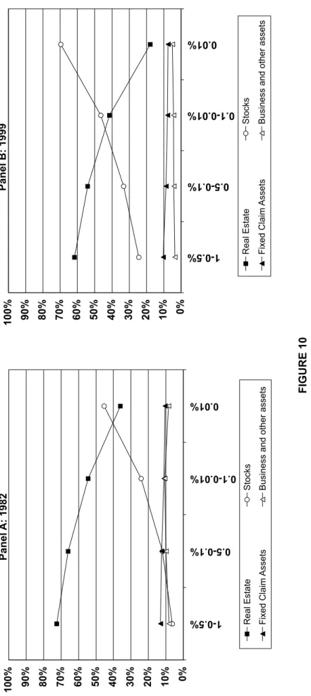
Figure 10 displays the composition of wealth in top fractiles of the wealth distribution in 1982 and 1999. As one would expect, the share of real estate is declining and the share of stocks is increasing as we move up the wealth distribution. It is notable that real estate still represents over 60% of wealth for the bottom half of the top percentile. Thus, only the very rich hold a substantial share of their wealth in the form of stock holdings. The patterns in 1982 and 1999 are quite similar except that the level of stock ownership is higher across the board in 1999, a year with high stock market prices. Those compositional patterns suggest that an increase in real estate price will benefit relatively less the very top and should therefore reduce the very top wealth shares. In contrast, an increase in stock prices will benefit disproportionately the very rich and should increase the very top wealth shares.

Figure 11 displays the top 1% wealth share (net worth including real estate wealth) along with the top 1% financial wealth share (net worth excluding real estate wealth and mortgage debts). Unsurprisingly, the top financial wealth share is larger than the top wealth share because financial wealth is more concentrated than real estate wealth. Top financial wealth concentration is stable around 25% from 1982 to 1990, decreases to about 21% from 1990 to 1995 and then increases again to about 26% by 2004. In contrast the top 1% wealth share including real estate is much more stable and fluctuates within a narrow band between 16 and 18 percent. In contrast to financial wealth, total wealth concentration does not fall from 1990 to 1995 because, as shown on Figure 9, real estate wealth also falls in that period,

and this advantages top wealth holders. The reverse happens from 1995 to 2004: in contrast to financial wealth, total wealth concentration does not increase because real estate prices increase sharply.

Figure 12 decomposes the top 1% total wealth share into three groups: the top 0.1%, the next 0.4%, and the bottom half of the top percentile. The graph shows that those top wealth groups have experienced different patterns. The top 0.1% share has fallen substantially from 8% in 1982 to 5% by 2004. In contrast, the top 1-0.5% has increased from 4.3 to 5.2 percent and the top 0.5-0.1% has slightly decreased from 7.6 to 7.2 percent. Those differential patterns are due primarily to composition effects: the bottom groups in the top percentile hold mostly real estate and have benefited from the surge in real estate prices. In contrast, the top 0.1% has been hit by the sharp real estate prices increases from 1986 to 1991 (see Figure 9). The improvement in real estate prices from 1997 to 2004 has been compensated by a surge in stock prices leading to an overall flat pattern for the top 0.1% wealth share during this period.

Figure 13 displays the wealth composition of top 0.1% wealth holders from 1982 to 2004. It shows that the shares of real estate, business assets, and fixed claim assets have been decreasing and that the share of stocks has been increasing but not enough to compensate for the fall in the other components. Therefore, over the last two decades, the dramatic increase in real estate prices has been the primary cause of the reduction in the concentration of wealth in Spain.

In 2002 the Bank of Spain conducted a household wealth survey whose preliminary results are presented in Bover, 2004. It is instructive to compare the wealth reported on wealth tax returns with the wealth reported in the survey. The complete comparison is reported in Table E3 in the appendix. Three important findings emerge.

First, we find that wealth reported on wealth tax statistics for top income groups such as the top 1% is higher than the wealth reported on the survey by the top 1%, even under the assumption that all the household wealth belongs to the head of household. For example, including real estate, the average top 1% wealth from tax returns is 1.8 million Euros while it is only 1.2 million in the survey. This shows that, in contrast to popular belief, it is not

clear that tax evasion for the wealth tax is pervasive as wealthy individuals seem to report more wealth for tax purposes than for the survey purposes.

Second, the total wealth reported in the survey (and especially financial wealth) is substantially lower than the aggregates from National Accounts that we use as the denominator. For example, the survey reports total wealth of about 2,000 billion Euros while National Accounts report total wealth of about 3,000 billions Euros. This suggests that households are under-reporting their wealth in the survey or that the survey might not have been sampled adequately to reflect a fully representative cross section of Spanish households.

Finally, because the gap in the aggregate between the survey and National Accounts and the gap for top groups between the survey and the wealth tax data are of comparable magnitude, our top wealth shares computed using wealth tax statistics and National Accounts for the denominator are relatively close to the top wealth shares computed internally from the survey (using as denominator total survey wealth).

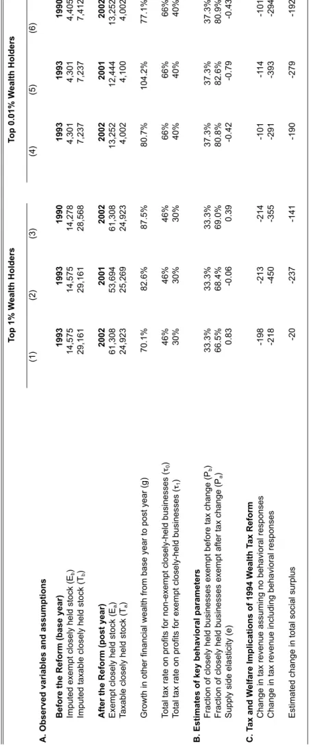
5. The Erosion of the Wealth Tax Base

In 1994, an exemption for business owners substantially involved in the management of their business was introduced in the wealth tax. More precisely, stocks of corporations where the individual owns at least 15%, or the individual and family own at least 20%, and where the individual is substantially engaged in this business activity (getting over 50% of his labor and business income from this activity) is exempted from the wealth tax. The value of those stocks still has to be reported to the fiscal administration and was included in our top wealth share series. The exemption was introduced in December 1993 for the first time, affecting wealth held by the end of 1994 (reported in 1995). Importantly for the empirical analysis below, the exemption criteria were relaxed for tax year 1995 (when the individual ownership

requirement was lowered from 20% to 15%) and in tax year 1997 (when the

20% family ownership criteria was introduced).30

5.1 Conceptual Model

In principle, the 1994 wealth tax reform could have two effects. First, the tax cut for exempted business might spur business activity in the exempted sector. We call this effect the supply side effect. Second, the tax cut for exempted business might induce some businesses, which did not originally meet the exemption criteria, to shift to the exempt sector in order to benefit from the tax cut. For example, business owners could increase their share of stock in the company in order to meet the 15% ownership threshold. Alternatively, they might become active managers in their businesses or drop other work activities outside the business. A business owner would be willing to shift to the exempt sector as long as the costs of shifting are less than the tax savings. We call this effect the shifting effect. In this subsection, we construct a simple model to capture those two effects and we propose an empirical application using our constructed wealth series in the following

subsection.31

We assume that business owners have an objective function of the form ! c " h(z) where ! z is pre-tax profits, !

c is net-of-tax profits, and

!

h(z) _{is an}

increasing and convex function representing the costs of earning higher profits. Those costs represent labor input costs (including the labor supply cost of the business owner if he is an active manager) and also capital input costs. The quasi-linear form of the objective function amounts to assuming away income effects or risk aversion effects, which simplifies the derivations

30 _{For tax year 2003 (beyond our study), the individual ownership requirement was further} reduced from 15% to 5%.

31 _{To the best of our knowledge, such a model has not been presented before in the literature} on the efficiency costs of taxation. It could be easily applied to other tax settings. For example, in the United States, the issue of shifting business profits from the corporate income tax base to the individual income tax base has received a lot of attention (see e.g., Slemrod, 1995, 1996, Gordon and Slemrod, 2000, Saez, 2004). Such shifting occurs because businesses meeting specific criteria (number of shareholders) can elect to be taxed directly at the individual level.

and the welfare analysis.32 _{Furthermore, we assume that the business owner}

can pay a cost

!

q " 0 in order to meet the tax exemption status. Such costs

represent for example the costs of increasing the business ownership to 15% or the opportunity costs of dropping outside work activities to meet the labor income requirement. We assume that

! q is distributed according to a cumulated distribution ! P(q). A fraction !

P0= P(q = 0) of businesses meet those

criteria even in the absence of the tax preference. In reality, businesses differ in size, which could be modeled through heterogeneity in the cost function

!

h(z)_{. However, as we consider only linear taxation (which is an approximation}

to the actual progressive tax system), the distribution of business sizes is irrelevant for the analysis and hence we assume that businesses differ only in

!

q.

We assume that the tax rate on profits

!

z in the taxed sector is

!

"0 and

that the tax rate in the exempt sector is

! "1 with of course ! "1#"0. Note that ! "1

is not necessarily zero as the business also faces corporate and individual income taxes. It is also important to note that we convert the wealth tax rate

!

t

into a tax rate

!

" on profits using the standard formula

!

"= t r where

!

r is the

normal annual return on assets. We denote by

!

l the tax status of the business

with

!

l = 0 denoting the standard taxable status and

!

l = 1 the exempt status.

The manager solves the following maximization problem:

!

max

l,z z(1"#l) " h(z) " q $ l

This maximization problem can be decomposed into two stages. First, conditional on ! l, ! z maximizes !

z(1"#l) " h(z) which generates the first order

condition

!

1"#l = h'(z). This equation captures the within sector supply side

effect, as a decrease in ! "l leads to an increase in ! zl with an elasticity ! e_l = 1"

(

₍

₎

)

₍

₎

(

( )

)

32 _{Including income effects would not change the qualitative nature of our findings but would} complicate the presentation, as we would have to introduce compensated elasticities to capture efficiency costs in our formulas. In the case of wealthy business owners who actively work in their business, it seems plausible to assume that income effects are small (if income effects were large, those business owners would not be working).

Second, the business chooses

!

l. We denote by

!

V_l = maxz

[

(

)

]

!

l = 0, 1 (not

including the cost

!

q of becoming tax exempt). Therefore, if

! q " V1# V0, then the exempt status ! l = 1 is optimal, while if ! q > V1" V0, then ! l = 0 is optimal. As a result, a fraction ! P*

= P(V1" V0) of businesses chooses the exempt status.

Using the envelope theorem, we have

! "Vl "#l = $zl. Therefore, ! "P* "#₀= p V

₍

₎

₍

₎

_{( )}

density of the distribution

!

P q

_{( )}

between the tax exempt and taxable status, then increasing the tax

!

"0 in the

taxable sector generates a shift toward the tax-exempt sector. Conversely, reducing the tax advantage of the exempt sector by increasing

!

"1 reduces the

number of firms in the tax-exempt sector. We denote by

!

T = 1" P

(

)

#1z1 the total tax revenue and by

!

W = 1" P

(

)

₍

₎

0 V1"V0

#

_{( )}

surplus is

!

SW = W + T . Routine computations show that:

! "T "#₀ = 1$ P *

(

)

(

)

(

)

The first term (equal to one) inside the square brackets of (1) and (2) represents the mechanical increase in tax revenue absent any behavioral response. The last two terms inside the square brackets represent the loss of tax revenue due to the supply side effect and the shifting effect respectively. The reduction in private surplus due to the tax change is equal to the

mechanical tax increase (absent behavioral responses).33 _{Therefore, the last}

two terms represent the net effect on social surplus SW of the tax increase or equivalently (minus) the marginal deadweight burden of increasing taxes. Absent shifting effects

!

p* = 0

showing that the marginal loss in tax revenue (per dollar) is proportional to the supply side elasticity

!

e and the tax rate

!

" . If the tax rate

!

"0 in the taxable sector is below the Laffer rate

maximizing tax revenue (when taking into account only supply side effects) then

!

"0z0>"1z1. Therefore, equation (1) shows that shifting effects increase

the marginal deadweight burden of increasing the tax in the taxable sector. In contrast, equation (2) shows that shifting effects decrease the marginal deadweight burden of increasing the tax in the exempt sector. The economic intuition is transparent: increasing the tax differential across the two sectors leads to more shifting: the marginal shifters spend

!

q for a tax saving equal to

!

q, which is pure deadweight burden. Strikingly, in the extreme case where

!

"1= 0,

34

!

"SW "#₁= p*#₀z₀ P*: social surplus increases with an increase in

!

"1

no matter how large the supply side effect in the tax exempt sector is. Therefore, providing a wealth tax exemption for businesses meeting some specific set of criteria has two opposite effects on social surplus. First, it has a positive effect on social surplus through the standard supply side effect: exempt businesses face lower taxes and hence might expand their economic activity. This effect is measured through the supply side elasticity

!

e. This

leads to an increase in business activity and hence reported business wealth in the exempt sector with no effect on the taxable sector. Second, however, the exemption might induce some businesses to shift to the exempt status and waste resources in doing so. This shifting effect leads to an increase in reported business wealth in the exempt sector, which comes at the expense of reported business wealth in the taxable sector. We propose an empirical estimation using our wealth composition series below.

5.2 Empirical Estimation

33 _{This can be seen directly from the fact that}

!

"Vl "#l = $zl, which is a direct consequence

of the envelope theorem.

34 _{As we discussed above, even though business owners benefiting from the exemption are} exempt from the wealth tax, business owners still pay income taxes on the profits so that in reality

!

Figure 14 displays the composition and share of financial wealth held by the top 0.01% wealth holders. Stocks are now divided into three components: publicly traded stock, taxable closely held stocks, and exempted closely held stock. In 1994, the first year the exemption was introduced, exempted stock represents only about 15% of total closely held stock reported by the top 0.01%. By 2002, the fraction has grown to 77%. Presumably, in 1994, individuals did not have time to reorganize substantially their business activity. Therefore, the 15% fraction of closely held stock benefiting from the exemption in 1994 must be close or just slightly above the fraction of closely held stock which would benefit from the exemption absent any behavioral

response to the introduction of the exemption.35 The fraction of business

exempt wealth grows enormously from 1994 to 2002, which is consistent either with a very large supply side effect or a significant shifting effect. However, the fraction of taxable closely held stocks shrinks significantly from 1994 to 2002 which strongly suggests that the great increase in tax exempt wealth comes, at least in part, at the expense of taxable wealth through the shifting channel. We use our series to quantify the relative size of each effect.

We propose a simple quantitative analysis using our estimated series and the model described above. Let us assume that, taking the tax or exempt status as fixed, business wealth is given by

!

z = z 1"

₍

₎

!

" is the total tax rate (including income and wealth taxes) on profits,

!

e is the supply side

elasticity, and

!

z is potential wealth absent any taxes. We assume that the

fraction of businesses in the tax-exempt sector is given by

!

P = P "

(

)

use subscript

!

b to denote before reform variables and subscript

!

a to denote

after reform variables. Hence

!

Pb is the fraction of businesses meeting the

exemption criteria just before the reform and

!

P_{a is the fraction of businesses}

meeting the exemption criteria after the reform. Hence

!

Pb " Pa captures the

shifting effect (purged from the supply side effect)

For a given top group (such as the top 1% or the top 0.01%), after the reform, we observe exempt closely held stocks

!

Paz a

(

)

and non-exempt

35 _{Those would be businesses for which the cost of shifting}

!

q was zero because the businesses already met the criteria.