HAL Id: halshs-00857945
https://halshs.archives-ouvertes.fr/halshs-00857945
Preprint submitted on 4 Sep 2013
HAL is a multi-disciplinary open access
archive for the deposit and dissemination of
sci-entific research documents, whether they are
pub-lished or not. The documents may come from
teaching and research institutions in France or
L’archive ouverte pluridisciplinaire HAL, est
destinée au dépôt et à la diffusion de documents
scientifiques de niveau recherche, publiés ou non,
émanant des établissements d’enseignement et de
recherche français ou étrangers, des laboratoires
Fair Retirement Under Risky Lifetime
Marc Fleurbaey, Marie-Louise Leroux, Pierre Pestieau, Grégory Ponthière
To cite this version:
Marc Fleurbaey, Marie-Louise Leroux, Pierre Pestieau, Grégory Ponthière. Fair Retirement Under
Risky Lifetime. 2013. �halshs-00857945�
WORKING PAPER N° 2013 – 31
Fair Retirement Under Risky Lifetime
Marc Fleurbaey
Marie-Louise Leroux
Pierre Pestieau
Grégory Ponthière
JEL Codes: I14, I18, J10, J22
Keywords: Risky lifetime, Mortality, Labour supply, Retirement, Compensation
P
ARIS
-
JOURDAN
S
CIENCES
E
CONOMIQUES
48, BD JOURDAN – E.N.S. – 75014 PARIS TÉL. : 33(0) 1 43 13 63 00 – FAX : 33 (0) 1 43 13 63 10
Fair Retirement under Risky Lifetime
Marc FLEURBAEY
yMarie-Louise LEROUX
zPierre PESTIEAU
xGregory PONTHIERE
{ kSeptember 4, 2013
Abstract
A premature death unexpectedly brings a life and a career to their end, leading to substantial welfare losses. We study the retirement deci-sion in an economy with risky lifetime, and compare the laissez-faire with egalitarian social optima. We consider two social objectives: (1) the max-imin on expected lifetime welfare (ex ante), allowing for a compensation for unequal life expectancies; (2) the maximin on realized lifetime welfare (ex post ), allowing for a compensation for unequal lifetimes. The latter optimum involves, in general, decreasing lifetime consumption pro…les, as well as raising the retirement age, unlike the ex ante egalitarian optimum. This result is robust to the introduction of unequal life expectancies and unequal productivities. Hence, the postponement of the retirement age can, quite surprisingly, be defended on egalitarian grounds –although the conclusion is reversed when mortality strikes only after retirement.
Keywords: risky lifetime, mortality, labour supply, retirement, com-pensation.
JEL codes: I14, I18, J10, J22.
The authors are grateful to Benoit Decerf for his comments on this paper.
yPrinceton University
zDép. des Sc. Economiques, ESG-Université du Québec à Montréal (UQAM), CIRPEE
(Canada) and CORE (Université catholique de Louvain, Belgium).
xUniversity of Liege, CORE, PSE and CEPR.
{Paris School of Economics and Ecole Normale Superieure, Paris. [Corresponding
au-thor]. Address: Ecole Normale Superieure, 48 bd Jourdan, 75014 Paris, France. E-mail: [email protected]. Tel: 0033-143136204.
kMarc Fleurbaey and Gregory Ponthiere acknowledge the …nancial support of the ANR
1
Introduction
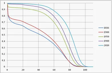
The continuous rise in life expectancy observed in industrialized economies in the last two centuries hides a fundamental feature of human life. Despite major advances in medical sciences, a human life remains a lottery, with a signi…cant variance in longevity outcomes. This point is well illustrated by survival curves, which give us the probabilities to reach all ages of life (based on the age-speci…c mortality rates prevailing at the year under study). As shown by Figure 1 for French males, provided mortality rates remain constant, more than 13 percent of the cohort born in 2010 will die before having reached the o¢ cial retirement age of 62 years.1 Moreover, about 20 percent will die before age 67.
Figure 1: Period survival curves: French males (1816 to 2010)
Average life expectancy statistics therefore hide this important uncertainty, and the induced inequalities in longevity outcomes. Only 61 percent of French males will reach the average life expectancy, equal to 78.04 years. The remaining 39 percent of the population will have a shorter life.
Those observations are not without consequences for optimal policy-making, in particular when considering the design of optimal pension system. From a policy perspective, the observed annual three-months increase in average life expectancy has often been used to justify postponing the legal retirement age in countries with Pay-as-You-Go pensions systems. Indeed, if individuals tend, "on average", to live longer, and if the retirement age remains the same, the sustainability of the pension system requires, under a constant fertility, either to increase the pension contributions, or to reduce the replacement ratio.2
The problem is that such a reasoning relies on a "on average" way of looking at things. In reality, there remain, as shown above, large longevity
inequali-1Sources: the Human Mortality Database (2013).
2On the potential gains from postponing the age at retirement, see Cremer and Pestieau
ties, and it is not at all clear that policy-makers should concentrate on average outcomes. An obvious reason why more attention should be paid to longevity in-equalities is that a signi…cant proportion of those inin-equalities are due to factors on which individuals have no in‡uence at all, and, thus, are circumstances for which agents can hardly be regarded as responsible.3 For instance, Christensen
et al (2006) claim that about one quarter to one third of longevity inequalities within a cohort can be explained by di¤erences in genetic background.
Given that longevity inequalities are, to a signi…cant extent, independent from individual behavior, there is a strong ethical support for a social security system that does not penalize the short-lived. The goal of this paper is to examine the design of the optimal retirement system in an economy with risky lifetime, with a social objective that incorporates a concern for inequalities.
In the context of risk, there are two main ways of taking account of in-equalities. One can …rst focus on inequalities in expected lifetime utility, and in particular give priority to people having lower life expectancy. This connects well to the policy proposal of making retirement age depend on working con-ditions which a¤ect longevity. But one can also look at the …nal distribution of longevity and realized utility across individuals, and thereby take account of the residual inequalities due to good or bad luck in the lottery of longevity. This relates to the policy discussions about giving less priority to the (lucky) elderly people who had their "fair innings". The former approach we call ex ante egalitarianism, and the latter ex post egalitarianism.
Here is a brief summary of our results. We …rst study the retirement decision in a two-period economy with identical agents and a risky lifetime. In such a simple framework, the laissez-faire allocation coincides with the ex ante egali-tarian social optimum, but not with the ex post egaliegali-tarian optimum because of the remaining longevity inequalities. The latter optimum involves a declin-ing consumption pro…le over the life cycle and a later retirement than in the laissez-faire. We then introduce inequalities in life expectancy which make the ex ante egalitarian approach depart from the laissez-faire, and show how the ex ante and the ex post approaches still di¤er signi…cantly. We …nally focus on the result that the ex post approach implies a later retirement, and we show that the opposite result can be obtained when mortality occurs mostly after retire-ment. The reason is that when mortality occurs early, a late retirement helps providing high consumption to the young, in order to help those among them who will have a short life. In contrast, when death strikes after retirement, it helps the short-lived to give them an early retirement. Finally, we study a more general model with wage heterogeneity and tax redistribution, and con…rm our results, qualitatively, in this setting.
In sum, the present paper suggests that adopting an ex post egalitarian social objective would lead to a strong reorganization of the lifecycle in terms of consumption and labour. As such, the present study complements the existing literature in several ways. First, it complements the existing positive literature
3See Fleurbaey (2008) on the distinction between circumstances and responsibility
on optimal labour and retirement age (see Sheshinski 1978, Crawford and Lilien 1981, Kahn 1988), by applying a model of labour and retirement decisions in a context of risky lifetime. Second, it also complements the normative literature on (socially) optimal labour and retirement age (see Cremer et al 2004), which relies on classical (Benthamite) utilitarianism, unlike the present, egalitarian ethical framework.4 Third, it complements recent attempts to apply ex post
egalitarian social criteria to economies with risky lifetimes (see Fleurbaey et al 2011), but which did not consider labor and retirement decisions.
The rest of the paper is organized as follows. Section 2 presents the basic framework where individuals who are identical ex ante turn out to have unequal longevity, and compares the laissez-faire with the social optimum under ex ante and ex post egalitarianism. Section 3 introduces unequal life expectancies and discusses several di¢ culties with the ex ante egalitarian approach. Section 4 studies the ex post approach under di¤erent assumptions about when mortality strikes in the lifecycle. Section 5 introduces a more general model with double heterogeneity: life expectancy and labour earnings. Section 6 concludes.
2
Identical individuals facing mortality risk
We consider a two-period model with risky lifetime. The population is a contin-uum of agents, with a measure normalized to 1. Agents live either one period or two periods. The old age (second period) is reached with a probability . During the young age (…rst period), agents supply their labour inelastically, consume and save resources for the old age. At the old age, agents can still work some subperiod, of length z, and are retired over the remaining subperiod of length 1 z.
We assume that lifetime welfare takes a time-additive form, and that old-age temporal welfare is additively separable in the utility of consumption and the disutility of labour. Assuming that agents have preferences satisfying the expected utility hypothesis, their preferences can be represented by:5
u(c) + [u(d) v(z)] ; (1)
where c and d denote …rst- and second-period consumptions, z denotes the retirement age, while u( ) is the temporal utility from consumption, whereas v( ) denotes the disutility of old-age labour. As usual, u( ) satis…es u0( ) > 0 and u00( ) < 0, and v( ) satis…es v(0) = 0, v0( ) > 0 and v00( ) > 0. Let u (c0) = 0
for a given c0> 0.
For analytical convenience, we assume that the labour market is perfectly competitive. Workers are paid at a wage rate w, which is taken as given by
4Utilitarianism also prevails in optimal retirement age studies in a dynamic setting (see
Michel and Pestieau 2002, Crettez and Le Maitre 2002, Lacomba and Lagos 2005).
5As usual, the utility of death is normalized to 0. Moreover, we assume away pure time
preferences for the simplicity of presentation. Note that the survival probability acts as a kind of "natural" discount factor.
them. There also exists a perfect annuity market, with actuarially fair returns. This amounts to assuming that consumption at the old age is:
d = Rs+ wz (2)
where R equals one plus the interest rate, while s denotes savings. For the sake of presentation, we will, throughout this paper, assume that R equals 1.
2.1
Laissez-faire and ex ante egalitarianism
In this simple setting, the laissez-faire allocation involves no ex ante inequality, and is therefore also the ex ante egalitarian optimum.
Agents choose their consumptions, savings and retirement age so as to max-imize their expected lifetime welfare subject to their budget constraint:
max
c;d;z u(c) + [u (d) v(z)]
s.t. c + d = w(1 + z) From the …rst-order conditions, we obtain:
u0(c) = u0(d) (3)
c = w(1 + z) d (4)
v0(z) = u0(d)w (5)
The laissez-faire involves a perfect smoothing of consumption across periods, i.e. c = d, as well as a retirement age such that the marginal disutility of old-age labour (LHS) equals the marginal welfare gain from working (RHS).
Let us provide the intuition for comparative statics with a few …gures. To study the impact of a change in , consider the following two equations, which derive from (4) and (5) after substituting c for d
c = w1 + z
1 + ; (6)
v0(z) = u0(c)w: (7)
From equation (7) one can write consumption as c = f (z), with f0(z) < 0 and
f00(z) > 0. This gives a decreasing convex curve (see Figure 2) that is intersected
by the line of equation (6) with intercept w= (1 + ) and slope w = (1 + ). When increases (raising life expectancy), only the budget equation (6) is a¤ected6 and this line goes down (its value at z = 1 remains unchanged, at w),
which implies that z goes up and c = d go down.
To study the impact of a change in w, consider the di¤erent system formed by (6) and the following equation, which derives from (7) after substituting w for its value in (6):
u0(c)c = v0(z)1 + z
1 + : (8)
6This, however, depends on our assumption of perfect annuities. Otherwise life expectancy
-z 6 c 6d 0 1 w 1+ w ? f (z) z c d
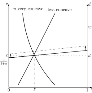
Figure 2: Impact of on laissez-faire
This equation provides a vertical line when u(c) = ln c; a decreasing curve if u is more concave than the logarithm, and an increasing curve when it is less concave than the logarithm (see Figure 3). In the former case, an increase in w, which raises the line of equation (6), triggers a decrease in z and an increase in c = d; in the latter case, provided that the curve of equation (8) is steeper than the line (6) at the intersection — this turns out to be always true— an increase in w triggers an increase in both z and c = d. When u(c) = ln c, z is una¤ected by a change in w.
As explained in the introduction, this allocation may not be satisfactory when it exhibits large welfare inequalities between the long-lived and the short-lived individuals. The latter’s lifetime welfare Usl equals u(c), whereas the
former’s lifetime welfare Ull equals 2u(c) v (z). Long-lived agents are better
o¤ than short-lived agents if and only if:
u(d) v(z) = u w(1 + z)
1 + v (z) > 0 (9)
that is, if the second period is worth being lived. We focus on this case here, and ignore the opposite case of poor economies in which it is a calamity to live in old age.
Let us brie‡y examine how this inequality depends on the parameters. As far as life expectancy is concerned, given that a rise in reduces d and raises z and, thus, v(z), it follows that lifetime welfare inequalities due to unequal lifetimes are smaller in economies with a higher expectancy.7
-z 6 c 6d 0 1 w 1+ w 6 6 u very concave less concave
z
c d
Figure 3: Impact of w on laissez-faire
When the e¤ect of productivity on retirement age is negative, or positive but small enough, a rise in w increases lifetime welfare inequalities between long-lived and short-lived.
The following proposition summarizes our results. Proposition 1 At the laissez-faire, we have:
c = d = w(1 + z) 1 + v0(z) = u0(d)w dz dw ? 0 () RR(c)7 1 dc dw = dd dw > 0; dz d > 0; dc d = dd d < 0;
where RR(c) = u00(c)c=u0(c) is the degree of relative risk aversion.
Long-lived agents enjoy a higher lifetime welfare than short-lived agents if and only if
u w(1 + z)
1 + v (z) > 0:
labour and less consumption at the old age, so that a premature death is necessarily less damaging there, in comparison with economies with worse survival conditions. This is, again, in‡uenced by the perfect annuity assumption.
Lifetime welfare inequalities between long-lived and short-lived are decreas-ing in life expectancy; they increase with productivity if
1
1 + 1 (1 + z)
v00(z)
v0(z) < RR(c):
Proof. See the Appendix.
Finally, note that, if the retirement age were …xed, i.e. z = z, then a rise in productivity would raise lifetime welfare inequalities between short-lived and long-lived, as this would increase consumption at the old age, and, hence, make premature death more damageable ceteris paribus. The endogeneity of the re-tirement decision prevents us from drawing such conclusions: agents may, under a higher productivity, work more or less, depending on whether the substitution e¤ect dominates the income e¤ect or not.
2.2
Ex post egalitarian …rst-best optimum
Let us now characterize the ex post egalitarian social optimum of this economy. Under this social objective, the social planner’s problem can be rewritten as:
max
c;d;zmin fu(c); u(c) + u(d) v(z)g
s.t. c + d = w(1 + z)
The objective function of that planning problem is continuous, but not dif-ferentiable. However, we can rewrite that problem in a simpler form assuming that the optimum features u(d) = v(z). This condition is necessary and su¢ -cient to insure the equality of lifetime welfare across individuals, whatever their longevity. Therefore, the social planner’s problem can be rewritten as maximiz-ing c under the constraints
u(d) = v(z)
c + d = w(1 + z):
This boils down to maximizing the quantity
c = w(1 + z) u 1 v (z) :
This is a concave function because u 1 v is convex. The …rst order condition
is
wu0 u 1 v (z) = v0(z) ; which is just (5) because u 1 v (z) = d.
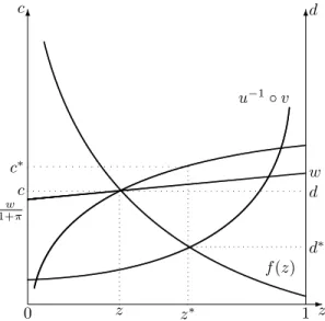
We focus on the case of an interior solution. As the FOC is just (5), it is easy to graphically compare the laissez-faire and the egalitarian optimum. From wu0(d ) = v0(z ), one derives d = f (z ), where, as in Figure 2, f (z ) =
u0 1(v0(z )=w), with f0(z ) < 0 and f00(z ) > 0. Moreover, c = w(1 + z ) d can be represented in the (z ; c ) space as a concave function c = w(1 +
z ) f (z ) that is below the line c = w(1 + z ) and has this line as an asymptote (see Figure 4).8 The socially optimum levels of d and z are obtained at the intersection of d = f (z ) and the egalitarian constraint u(d ) = v(z ), rewritten as d = u 1 v(z ).9 Given that lim
z!0f (z) > limz!0u 1 v(z) and
limz!1f (z) < limz!1u 1 v(z), such an intersection always exists. Then, for
that level of z , we obtain, from c = w(1 + z ) f (z ), the socially optimal consumption c . -z 6 c 6d 0 1 w 1+ w f (z) u 1 v z c d z c d
Figure 4: Comparing laissez-faire and social optimum
The ex post egalitarian optimum can be compared with the laissez-faire as follows. At the laissez-faire, the optimal level of z is characterized by the intersection of the decreasing curve d = f (z) with the increasing concave curve c = w(1 + z) f (z). On the contrary, at the ex post egalitarian optimum, the optimal level of z is determined by the intersection of d = f (z) with the increasing convex curve d = u 1 v(z). The intersection between d = f (z)
with d = u 1 v(z) is, in general, on the south east of the intersection between
d = f (z) and c = w(1 + z) f (z).10 Hence the retirement age at the ex post
egalitarian optimum exceeds its laissez-faire level, and that old-age consumption is lower than at the laissez-faire, whereas young age consumption is higher than at the laissez-faire. The following proposition speci…es our results.
Proposition 2 Comparing the ex post egalitarian optimum ( ) with the laissez-faire, if u(d) > v(z) at the laissez-laissez-faire, then:
c > c = d > d ; z > z:
8Observe that the curves of equations c = w(1 + z) f (z), c = f (z), and c = w(1 +
z)=(1 + )intersect at the same point.
9Note that, if z = 0, d = u 1(0) = c 0> 0: 1 0Exceptions include very poor economies (see supra ).
Proof. Both the laissez-faire and the egalitarian optimum satisfy
c = w(1 + z) f (z)
d = f (z);
where f (z) = u0 1(v0(z)=w). The …rst expression is increasing in z whereas the
second is decreasing. Therefore, c > c and d < d if and only if z > z: The laissez-faire, in addition, satis…es c = d; in contrast, the egalitarian optimum has u(d ) = v(z ).
At the laissez-faire, one therefore has w(1 + z) f (z) = f (z), i.e., f (z) = w(1 + z)= (1 + ). At the egalitarian optimum, one has u(f (z )) = v(z ), i.e., f (z ) = u 1 v(z ).
Under the assumption that u(d) > v(z) at the laissez-faire, then w(1 + z)= (1 + ) > u 1 v(z), which implies that f (z) > u 1 v(z). As f is
decreasing and u 1 v is increasing, the equation f (z ) = u 1 v(z ) requires
z > z.
The proof actually shows an "if and only if" fact: if u(d) < v(z) at the laissez-faire (a poor economy), then the inequalities are reversed, and the egalitarian optimum transfers resources from the young to the old in order to make life bearable in old age: c < c, d > d and z < z.
Hence, in the case of a- uent economies, ex post egalitarianism involves longer lifetime working periods. This somewhat counterintuitive result can be explained as follows. From an ex post egalitarian perspective, the only thing that matters is to maximize the welfare of the worst-o¤. In advanced economies with a su¢ ciently large output, the worst-o¤ is, unambiguously, the short-lived. Therefore, if one wants to minimize ex post welfare inequalities, all resources need to be targeted towards the short-lived individuals. Given that those can hardly be identi…ed ex ante, nor compensated after their death, the only solution is to allow young age consumption that is as large as possible. This is achieved by making the surviving old work longer than at the laissez-faire.
This has some consequences when one thinks about the direction of intertem-poral resource transfers, that is, the issue of positive or negative savings. The laissez-faire is characterized by positive savings, since c = w(1+ z)1+ < w for ; z < 1, leading to a transfer of resources from the young age of life towards the old age. On the contrary, under the ex post egalitarian optimum, the direc-tion of intertemporal resources transfers is the opposite: from old age towards the young age. Indeed, from the budget constraint, we have:
c = w + (wz d )
The curve of equation d = wz is an increasing linear curve that lies above the curve u(d) = v(z) at z = z if w is high enough, so that the factor (wz d ) is then positive, which implies the occurrence of negative savings. Thus, the ex post egalitarian optimum involves intertemporal transfers from the old age towards the young age, in su¢ ciently productive economies.
If, for some reason (e.g., political constraints), intertemporal transfers from the old age towards the young age are not possible, one can seek to obtain
a constrained egalitarian optimum, which has c = w and d = wz. One can show that z is then at an intermediate value between the laissez-faire and the unconstrained optimum. Inequalities are then not fully eliminated and long-lived agents are now better o¤ than the short-long-lived.
3
Unequal life expectancies
Not all human activities are characterized by the same mortality risks. Blanpain (2011) shows that, in France (2000-2008), life expectancy at age 35 is equal to 40.9 years for a blue collar, against 47.2 years for an executive. In this light, it makes sense to explore what our results become under unequal life expectancies. For this purpose, we introduce two kinds of individuals, with unequal mor-tality risks, in the two-period model:
Type-H agents, who have a high life expectancy 1 + H;
Type-L agents, with a lower life expectancy 1 + L, with L< H.
For simplicity, we assume that there exists an equal proportion of type-H agents and of type-L agents in the population (at the young age). We also assume that there exist type-speci…c annuity markets for the two types of in-dividuals. Hence type-i agents who survive to the old age bene…t from savings returns equal to 1
i.
3.1
Laissez-faire
In the laissez-faire, individuals of type i 2 fH; Lg face the following problem: max
si;zi u(w si) + i u
si i
+ ziw v(zi)
The FOCs are:
u0(ci) = u0(di) (10)
v0(zi) = u0(di)w (11)
From Prop. 1, we directly deduce that: cL= dL= w(1 + zL L) 1 + L > cH = dH = w(1 + zH H) 1 + H and that zL< zH.
Thus, type-L agents enjoy higher consumption at all periods and retire ear-lier. Despite this, type-L agents may have a lower expected utility, due to their greater mortality, i.e., it is possible to have
u(cH) + H[u (cH) v(zH)] > u(cL) + L[u (cL) v(zL)]
Proposition 3 At the laissez-faire, if u(cH) v(zH) > maxz2[zL;zH]v0(z)(1
z)= (1 + L), then
u(cH) + H[u (cH) v(zH)] > u(cL) + L[u (cL) v(zL)] :
Proof. Consider the comparative statics of Prop. 1. The expression u(c) v(z) is decreasing in . Therefore if u(cH) v(zH) > maxz2[zL;zH]v0(z)(1
z)= (1 + L), one has u(c) v(z) > v0(z)(1 z)= (1 + ) for all 2 [ L; H].
The expression u(c) + [u (c) v(z)] is increasing in if (1 + ) u0(c)dc
d v
0(z)dz
d + u (c) v(z) > 0: Using wu0(c) = v0(z), one obtains
u0(c) (1 + ) dc
d w
dz
d + u (c) v(z) > 0:
One has c = w(1 + z)= (1 + ). The expression in bracket is therefore equal to (1 + ) dc d w dz d = (1 + ) [ w(1 + z) (1 + )2 + wz 1 + + w 1 + dz d ] w dz d = [w (1 z) = (1 + )] :
The result is obtained by using wu0(c) = v0(z) once again.
Observe that it is not su¢ cient to have u(c) v(z) > 0 to make it a bene…t to have greater life expectancy. The reason is that with perfect annuities, the rate of return on savings decreases, making the initial consumption-labour bundle una¤ordable after an increase in . If we assumed that all agents faced the same rate of return, then it would be easier to obtain inequalities in expected utility to the bene…t of the agents with greater life expectancy.
3.2
Ex ante egalitarian optimum
A social planner whose aim is to maximize the minimum expected lifetime welfare faces the following problem:
max
ci;di;zimin fu(cH) + H[u (dH) v(zH)] ; u(cL) + L[u (dL) v(zL)]g
s.t. X i=H;L [ci+ idi] = X i=H;L [w + wzi]
We can thus reformulate the social planner’s problem as follows: max
ci;di;zi [u(cL) + L[u (dL) v(zL)]] + (1 ) [u(cH) + H[u (dH) v(zH)]]
s.t. X i=H;L [w + iwzi] X i=H;L [ci+ idi] = 0
where is set so as to ensure that we obtain:
[u(cL) + L[u (dL) v(zL)]] = u(cH) + H[u (dH) v(zH)]
We obtain the following …rst-order conditions:
u0(cL) = u0(dL) = (12)
u0(cH) = u0(dH) =
1 (13)
v0(zL) = u0(dL)w (14)
v0(zH) = u0(dH)w (15)
Under the objective of maximizing the utility of the worst-o¤ agent, and assuming that the type-L agent is the worst o¤, we have that > 1 , so that type-L consumptions are larger than the ones of a type-H agent.
We thus have consumption smoothing, but at di¤erent levels for the two types of agents. Type-L agents enjoy higher consumption at the two periods. Hence, from the last two FOCs, it follows also that type-H agents should also work longer, and retire later than type-L agents, on the grounds of the equal-ization of expected lifetime welfare.
Proposition 4 Under H > L, the ex ante egalitarian optimum involves:
cL = dL> cH= dH
zL < zH Proof. The proof follows from the FOCs.
Thus, at the ex ante egalitarian optimum, individuals with lower survival chances should consume more than individuals with high survival chances, and retire earlier than these. Unequal consumption patterns and retirement ages are indeed the only way to yield an equalization of expected lifetime welfare across groups with unequal survival prospects.
Let us mention that, under asymmetric information, there would be a con-‡ict between the ex ante egalitarian constraint and the incentive compatibility constraint. Indeed, if the social planner cannot observe individual survival prob-abilities, and proposes the …rst-best contracts, type-H agents have an interest in claiming to be type-L ones. Hence, under asymmetric information, one needs to add an incentive constraint of the form,
u(cH) + H[u (dH) v(zH)] [u(cL) + H[u (dL) v(zL)]] 0 (16)
to the …rst-best problem so as to prevent mimicking from type-H agents. In equi-librium, this constraint is binding and no contract f(cL; dL; zL) ; (cH; dH; zH)g
can satisfy both the incentive compatibility constraint (16) and the egalitar-ian constraint. There is thus a con‡ict between egalitaregalitar-ianism and incentive compatibility.
This analysis reveals two problems with ex ante egalitarianism.11 First, equalizing expected lifetime welfare across groups with di¤erent life expectancies may still leave large ex post welfare inequalities between long-lived and short-lived individuals. Indeed the above allocation of resources only equalizes the expected lifetime utility across groups, but there still remain large inequalities within groups, as a consequence of unequal lifespans.
The second problem is perhaps less apparent, but no less deep. It is assumed here that H, L are simultaneously the average survival rate in the two
sub-groups and the individual survival probability of each member of the group. In real-life applications, this assumption never holds. The average life expectancy of blue-collar workers is not the individual life expectancy of every blue-collar worker. It is in fact deeply problematic for the ex ante egalitarian approach to require de…ning individual life expectancies. First, individuals may not be trusted to have the best estimate of their own life expectancy, because average subjective life expectancy generally di¤ers from observed average life expectancy (Brouwer and van Exel 2005). Second, the very notion of an individual life ex-pectancy is problematic. In a deterministic world, individual life exex-pectancy and individual …nal longevity coincide. The ex post approach, by focusing on the distribution of actual longevities, may in fact be the best version of the ex ante approach, because it relies on the true individual life expectancy, not on subgroup average life expectancy. In a sense, the ex ante egalitarian approach remains utilitarian at the subgroup level (individual expected utility being abu-sively proxied by subgroup average utility). In welfare economics, individualistic approaches are better. If inequality aversion is introduced, it should be at the individual level, not at the subgroup level. Therefore, from now on we focus mainly on the ex post approach.
3.3
Ex post egalitarian optimum
From an ex post perspective, the planner’s problem is: max ci;di;zimin U ll H; UHsl; ULll; ULsl s.t. X i=H;L [ci+ idi] = X i=H;L [w + iziw]
We can rewrite the social planning program in a more convenient way, by adding egalitarian constraints. Three egalitarian constraints are needed: two constraints guaranteeing that long-lived and short-lived agents for a given type are equally well:
u (dL) v(zL) = u (dH) v(zH) = 0;
and one additional constraint guaranteeing that individuals with some equal longevity are equally well-o¤ across ex ante types: u(cH) u(cL) = 0. The
latter implies cH = cL = c .
1 1Additional rationality arguments against ex ante egalitarianism (i.e., it violates statewise
The budget constraint, supplemented with the egalitarian constraints, im-plies
2c = w (2 + HzH + LzL) Hu 1 v (zH) Lu 1 v (zL ) :
Maximizing c under this constraint implies w = u 1 v 0(z
H) = u 1 v
0(z L) :
Therefore, zH = zL , hence dH = dL. The two subgroups have the same consumption-labour bundle, independent of their survival rate:
c > dH = dL
zH = zL
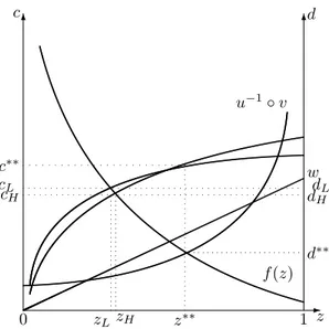
We thus have an equal optimal age at retirement, as well as equal old-age consumptions, which are inferior to …rst-period consumption.12
To compare this with the laissez-faire, remember …rst that the ex post egali-tarian optimum z is obtained as the intersection of the f curve d = f (z) with the egalitarian constraint d = u 1 v(z). This intersection determines d
i and
zi for the two types, which can then be substituted in the resource constraint, to obtain …rst-period consumptions, i.e., 2c = w(2 + Lz + Hz ) ( L+
H)f (z ).
The laissez-faire equilibrium is represented as the intersection of the f curve with the corresponding c curves, i.e. ci = w(1 + izi) if (zi). Observe that
the previous curve for c is the average of these two curves.
From Proposition 2 it is clear that, if u(dH) > v(zH) (which implies u(dL) >
v(zL)), cL = cH > cH, dL = dH < dH < dL, and zL = zH > zH > zL, but
the comparison between cL and cL (which is greater than cH) is ambiguous.
However, if one assumes that at the egalitarian optimum, wz > d , then z is greater than the solution z+ to wz+ = f (z+): At z+, the two curves
c = w(1 + iz) if (z) cross. When z > z+ > z, therefore, necessarily
c > cL; cH, as can be seen from Figure 5.
The following proposition summarizes our results.
Proposition 5 The ex post egalitarian optimum involves: cL = cH > dL = dH
zL = zH:
In comparison to the laissez-faire, assuming that u(dH) > v(zH), we have:
cL = cH > cH
dL = dH < dH < dL
zL = zH > zH > zL:
1 2As above (section 2.2), we focus here on the case of su¢ ciently rich economies. In very
poor economies, the optimal lifecycle consumption pro…le would be increasing rather than decreasing, as the low productivity level would not allow for u(di) v(zi) 0.
-z 6 c 6d 0 1 w f (z) u 1 v zH zL cH dH cL dL z c d
Figure 5: Comparing laissez-faire and social optimum If, in addition, one assumes that wz > d , we have:
cL = cH > cL> cH:
Proof. See above.
In sum, the introduction of unequal life expectancies does not a¤ect the ma-jor features of the ex post egalitarian optimum. Note also that this allocation is still implementable under asymmetric information, as the allocation is inde-pendent of the survival probabilities. In comparison to the ex ante egalitarian optimum, the ex post egalitarian optimum recommends more consumption at the young age (except possibly for type L), and less consumption at the old age. Moreover, the optimal retirement age is also later under the ex post egalitarian optimum than under the ex ante egalitarian optimum. Thus, adopting an ex post view leads to a deterioration of the living conditions of surviving type-L agents, that is, of lucky, long-lived agents who faced initially a lower life ex-pectancy, as well as a widening of consumption possibilities for type-H agents at the young age, on the grounds of a possible premature death even within the type-H group.
4
Egalitarianism and retirement age
The conclusion that egalitarian concerns require postponing retirement is driven by the fact that the worse-o¤ are individuals who die before retiring. The most one can do for them is to increase their consumption, and to this e¤ect it is ben-e…cial if the lucky long-lived work even more to provide for more consumption resources to transfer to the young.
This reasoning may not be very robust. It might be possible to improve the lot of the disadvantaged by granting them early retirement. This section explores variants of the model in which this opposite conclusion may arise.
The idea is to introduce three periods so that mortality may be described as striking primarily before or after retirement. Let us now assume that agents work in the …rst and second periods, retire during the second period and then, if still alive, enjoy their retirement in the third period. The probability to reach period 2 is now denoted by 2, whereas the probability to reach the old age,
conditionally on survival to period 2, is denoted by 3.
4.1
Laissez-faire
At the laissez-faire, the individual problem is now: max s1;s2;z u(w s1) + 2 u s1 2 + zw s2 v (z) + 2 3u s2 3
where s1, s2 denotes …rst- and second-period savings. Assuming an interior
solution, the FOCs can be rewritten as:
u0(c) = u0(d) = u0(b) (17)
v0(z) = u0(d)w (18)
c = w(1 + 2z) 2d 2 3b (19)
where b is third-period consumption. We thus have a perfect consumption smoothing across periods. Substituting in the budget constraint yields:
c = d = b = w(1 + 2z)
1 + 2+ 2 3
One can thus represent the laissez-faire as the intersection, in the (z; c) space, of the increasing line c = 1+ 2+w
2 3 + w 2
1+ 2+ 2 3z with the decreasing curve
d = f (z) obtained from v0(z) = u0(d)w. A rise in productivity w pushes the d curve up, and raises both the intercept and the slope of the c line. Hence, it contributes to increase consumption, but has an e¤ect on retirement age that depends the elasticity of u0, as in Prop. 1. A rise in
2 leaves the function
d = f (z) unchanged, but lowers the c line, implying a later retirement age, as well as a lower consumption (see Figure 2 — the only di¤erence here is that the …xed point of the c line when 2changes occurs for z = 1 + 3instead of z = 1).
Similarly, a rise in 3 leaves the function d = f (z) unchanged, and lowers the c
line, implying a higher z, as well as a lower consumption. Thus changes in 2
and 3have qualitatively similar e¤ects on retirement age at the laissez-faire.
Regarding welfare inequalities, individuals who live the maximum length of life are better o¤ than those who die after the second period if and only if:
u w(1 + 2z)
1 + 2+ 2 3
Moreover, individuals who live only two periods are better o¤ than those who live only one period if and only if:
u w(1 + 2z)
1 + 2+ 2 3
v(z) > 0
From this, it follows that, if agents who live only two periods are better-o¤ than those who live only 1 period, agents living the maximum life will also be better o¤ than those living the minimum life. When considering lifetime welfare inequalities between agents with di¤erent longevity, it appears that a rise in productivity, by raising consumption at all ages of life, raises the welfare inequalities between those living three periods and those living only two periods. A rise in 2, by implying a later retirement and a lower consumption, will
reduce welfare inequalities between those living only one period and the other individuals, who enjoy longer lives. The same is true for a rise in 3.
Proposition 6 At the laissez-faire, we have:
c = d = b = w(1 + 2z) 1 + 2+ 2 3 v0(z) = u0(d)w dz dw 7 0; dz d 2 > 0; dz d 3 > 0
Agents with the minimum longevity are the worst-o¤ if and only if
u w(1 + 2z)
1 + 2+ 2 3
v (z) > 0
Lifetime welfare inequalities between agents living 3 periods and agents living 1 period are increasing in w, but decreasing in 2 and 3.
Proof. See the Appendix.
4.2
Egalitarian …rst-best optimum
Here again, we will not focus on the ex ante egalitarian optimum, which yields the same allocation as the laissez-faire, and focus instead on the ex post welfare of the worst-o¤ individual.
Note that, under 2< 1, that egalitarian constraint includes two parts:
u(d) v(z) = 0 and u(b) = 0
The …rst part states that individuals living one more period are not better o¤ than those who die after period 1, whereas the second part states that individu-als living two more periods are not better o¤ either. This implies that b = c0.
agents who live two periods and those who live only one. As in the previous section with only two periods, the social planning problem can be written in a simple form:
max
z c = w (1 + 2z) 2u
1 v (z)
2 3c0:
As far as z is concerned, this boils down to maximizing w (1 + 2z) 2u 1
v (z), a problem that has already been studied in Subsection 2.2. If 2< 1, we
thus obtain a decreasing consumption pro…le over the lifecycle:13
c > d > b = c0:
But let us now examine the special case in which there is no premature death during the career, so that 2= 1. In that case, the egalitarian constraint is only
u(b ) = 0, leading to b = c0. Hence the social planner’s problem becomes:
max
c;d;zu(c) + u(d) v(z) + [w + zw c d 3c0]
where is the Lagrange multiplier associated to the resource constraint of the economy. Hence the FOCs are now:
u0(c ) = u0(d ) (20)
v0(z ) = u0(d )w (21)
w + z w = c + d + 3c0 (22)
From which we now have:14
c = d > b = c0
Hence, in that case, there is perfect consumption smoothing during the active life (1st and 2nd life-periods), which is akin to what happens in the laissez-faire. But c = d are greater than at the laissez-faire (in a- uent economies), because they determine the well-being of the short-lived. Given the relationship v0(z ) = u0(d )w, a greater d implies a lower z : Therefore we now obtain that optimal retirement occurs earlier than at the laissez-faire.
This result can be understood as follows. As death strikes only during re-tirement, the goal is to enhance the well-being of the active and the young pensioners. As e¢ ciency requires retirement to occur when working more has a marginal disutility equal to the marginal utility of the consumption it pays, a better situation for these people means that they have a lower marginal utility of consumption, therefore should stop working before marginal disutility rises
1 3We leave aside the extreme case of very poor economies, where the low productivity
level would always make the long-lived worse o¤ than the short-lived, and where the ex post egalitarian optimum would involve an increasing optimal consumption pro…le, contrary to what prevails under non-poor economies.
1 4Once again, we assume here that the productivity level is su¢ ciently large, so as to allow
too much. Their extra welfare (compared to the laissez-faire) is split between extra consumption and extra leisure.
In sum, the extent to which the egalitarian optimum di¤ers from the laissez-faire depends on the timing of premature deaths. If premature deaths occur during the career, the retirement age should be postponed from an egalitarian perspective. However, if death only arises at the end of the career, then the retirement age should be advanced.
Proposition 7 Suppose that 2< 1. Comparing the ex post egalitarian
optimum ( ) with the laissez-faire, we have:
c > c; d < d; b < b; z > z
Suppose that 2 = 1. Then, comparing the ex post egalitarian optimum
( ) with the laissez-faire, we have:
c > c; d > d; b < b; z < z Proof. See above.
In any case, consumption at the young age is always too low at the laissez-faire in comparison with the ex post egalitarian optimum. But the crucial di¤er-ence lies in the treatment of individuals in the second part of their career. The ex post egalitarian optimum recommends to reduce their consumption and to postpone their retirement with respect to the laissez-faire when some premature deaths occur during the active life, whereas it recommends the opposite when death only occurs once the career is fully completed. Our advanced societies are still very much concerned with the …rst case, but, over time, may come closer and closer to the second case, as illustrated on Figure 1 for French males.
4.3
Moderate egalitarianism
The above analysis reveals a tension between the interests of the very worse-o¤ who die at the end of the …rst period, and for whom increasing consumption (therefore postponing retirement) is bene…cial, and the slightly less disadvan-taged who die one period later and would bene…t from earlier retirement.
Full egalitarianism focuses only on the very worse-o¤, but if one considered a moderate form of egalitarianism, it may happen that the fate of the less disadvantaged looms larger, for instance if they are su¢ ciently many while the worse-o¤ are few. It is therefore worth exploring the possibility to obtain a policy of early retirement even when mortality strikes at all periods, provided that mortality in period 2 is small and that the degree of priority for the worse-o¤ is moderate.
A moderate egalitarian social planner seeks to maximise the following social welfare function, where G( ) is an increasing concave transform:
subject to the following resource constraint:
w (1 + 2z) c + 2d + 2 3b
The …rst order conditions of this problem are written as follows: @$ @c = [(1 2)G 0(U 1) + 2(1 3) G0(U2) + 2 3G0(U3)]u0(c) = 0 @$ @d = [(1 3) G 0(U 2) + 3G0(U3)]u0(d) = 0 @$ @b = G 0(U 3) u0(b) = 0 @$ @z = [(1 3) G 0(U 2) + 3G0(U3)] v0(z) + w = 0
where Ut is the ex post utility of an agent living t = 1; 2; 3 periods of life:
U1= u(c); U2= u(c) + u(d) v(z); U3= u(c) + u(d) v(z) + u(b).
The above FOCs do not allow us to draw unambiguous results about the form of the moderate egalitarian optimum. In the following, we provide a numerical example aimed at comparing the moderate egalitarian optimum with the full egalitarian optimum. To do so, we use the following functional forms: u (c) = ln(c), v(z) = 2z2 and G(u(x)) = u(x)"
" . We also assume that w = 10 and 2 = 0:9 and 3 = 0:8. We make the parameter of inequality aversion " vary
between 1 and 30.15 The following table contrast the laissez-faire (Section 4.1)
with the full egalitarian optimum (Section 4.2) and the moderate egalitarian optimum, under di¤erent degrees of inequality aversion.
LF Moderate Egalitarianism Full Egalit.
" 1 0.5 0.1 -0.5 -1 -2 -3 -10 -30 c 5.41 5.41 5.67 5.93 6.40 6.85 7.76 8.58 11.30 12.58 13.26 d 5.41 5.41 5.37 5.32 5.21 5.09 4.83 4.58 3.78 3.43 3.25 b 5.41 5.41 5.12 4.87 4.48 4.15 3.55 3.07 1.74 1.23 1.00 z 0.46 0.46 0.47 0.47 0.48 0.49 0.52 0.55 0.66 0.73 0.77 U1 1.69 1.69 1.73 1.78 1.86 1.92 2.05 2.15 2.42 2.53 2.59 U2 2.95 2.95 2.98 3.01 3.05 3.07 3.09 3.08 2.88 2.70 2.59 U3 4.63 4.63 4.62 4.59 4.55 4.49 4.35 4.20 3.43 2.91 2.59
Under full and moderate egalitarianism, …rst-period consumption should be increased with respect to the laissez-faire, whereas second- and third-period consumptions should be decreased.16 However, the extent to which optimal and
laissez-faire levels di¤er depends on the degree of aversion toward inequality: the di¤erence between …rst-period and subsequent-periods consumption levels is maximum under full egalitarianism, but decreases as " increases.
1 5Assuming " = 1 under moderate egalitarianism is equivalent to assuming a utilitarian
social planner maximising ex ante utilities.
Regarding the optimal retirement age, we also obtain that, under moderate egalitarianism, the optimal z increases with the degree of inequality aversion. To interpret those results, one can assume that each period lasts 25 years, with the active life starting when the individual is aged 25. At the laissez-faire, the age at retirement is equal to about 61.5 years. When " is remains high, the optimal retirement age under moderate egalitarianism is close to the one at the laissez-faire. For instance, the optimal age at retirement when " = 1 is equal to about 62.5 years. The largest retirement age under moderate egalitarianism, obtained under " = 30, is equal to 68.25 years. This remains below the optimal retirement age under full egalitarianism, which is equal to 69.25 years. The underlying intuition behind those higher retirement ages under a higher inequality aversion is the following: making individuals work longer tends to reduce the welfare di¤erentials between those who live a short life and those who enjoy a longer life. Note, however, that the optimal retirement age remains, even under full egalitarianism, limited, because of the high desutility of old-age labour postulated in this numerical example.
Note also that, while inequalities in utilities between individuals living one, two and three periods are maximum under the laissez-faire and utilitarianism, those inequalities are reduced as inequality aversion increases. Under full egal-itarianism, we …nd, not surprisingly, that ex post utilities are equalized across individuals having unequal realized longevity.
How would an improvement of survival conditions a¤ect the social optimum under moderate and full egalitarianism? To answer that question, the following table shows the laissez-faire, the moderate egalitarian optimum and the full egalitarian optimum when 2 is as high as 0:99.
LF Moderate Egalitarianism Full Egalit.
" 1 0.5 0.1 -0.5 -1 -2 -3 -10 -30 c 5.28 5.28 5.36 5.43 5.56 5.68 6.01 6.43 9.63 12.16 13.59 d 5.28 5.28 5.33 5.36 5.41 5.45 5.47 5.43 4.46 3.65 3.25 b 5.28 5.28 5.07 4.90 4.62 4.38 3.91 3.47 1.90 1.25 1.00 z 0.47 0.47 0.47 0.47 0.46 0.46 0.46 0.46 0.56 0.68 0.77 U1 1.66 1.66 1.68 1.69 1.71 1.74 1.79 1.86 2.26 2.50 2.59 U2 2.88 2.88 2.91 2.94 2.98 3.01 3.08 3.13 3.13 2.86 2.59 U3 4.54 4.54 4.53 4.52 4.51 4.49 4.44 4.37 3.77 3.08 2.59
An interesting result concerns the optimal age at retirement. At the laissez-faire, the age at retirement is now larger than under 2= 0:9. However, under
full egalitarianism, the optimal age at retirement remains, under 2 = 0:99,
exactly the same as under 2= 0:9, and equal to 0.77 (or, in usual units, 69.25
years). On the contrary, under moderate egalitarianism, the optimal retirement age is, under 2 = 0:99, signi…cantly lower than under 2= 0:9. Hence, while
an improvement in survival conditions makes individuals work longer at the laissez-faire, the two kinds of egalitarian optima have very di¤erent implications in terms of the optimal age at retirement.
In sum, this non-exhaustive numerical illustration shows that moderate egal-itarianism involves, depending on the degree of inequality aversion, a large span of intermediate social optima including di¤erent optimal retirement ages -between two extreme situations: on the one hand, the laissez-faire (equivalent here to the utilitarian optimum), and, on the other hand, the full egalitarian optimum. Moreover, an improvement of survival conditions is shown to have quite distinct e¤ects on the optimal age at retirement under the laissez-faire and under the two egalitarian optima considered. While raising 2 leaves the
optimal age at retirement unchanged under full egalitarianism, this raises the re-tirement age at the laissez-faire and reduces the rere-tirement age under moderate egalitarianism.
5
Unequal life expectancy and productivity
Whereas the previous sections relied on a unique source of heterogeneity ex ante - unequal life expectancy -, let us conclude this study by studying the dou-ble heterogeneity case, where both individual survival prospects and individual productivities di¤er. For that purpose, we turn back to the baseline 2-period model, but introduce four types of agents ex ante, who di¤er in their survival type i 2 fH; Lg and in their productivity type j 2 fh; `g. We have:
H > L
wh > w`
Hence, there exist four distinct groups of agents ex ante: types Hh, H`, Lh and L`. For simplicity, we assume that there exists an equal proportion of the four types of agents in the population (at the young age).
5.1
Laissez-faire
As in the previous sections, there exists a perfect annuity market, which yields a return on annuities, 1= i where the gross interest rate is R = 1. Individuals
of type fi; jg face, at the laissez-faire, the following problem: max
sij;zij u(wj sij) + i u
sij i
+ zijwj v(zij)
and the FOCs are:
u0(cij) = u0(dij) (23)
v0(zij) = u0(dij)wj (24)
As in the previous cases, consumption should be equalized across time so that cij= dij=
wj(1 + zij i)
1 + i
Using the results of Proposition 1, we obtain the following ranking cLh = dLh> cHh= dHh cL` = dL`> cH`= dH` cLh = dLh> cL` = dL` cHh = dHh> cH`= dH` or equivalently cLh> cHh? cL`> cH`
The ranking of retirement ages follows that of Proposition 1 so that dzij=dwj7 0
(depending on the value of RR(c))) and dzij=d i> 0. Hence, it is not possible
to have a complete ranking of the retirement ages as a function of the di¤erent sources of heterogeneity. Only it is possible to show that:
zHj> zLj 8j 2 fh; `g
Long-lived agents are better o¤ than short-lived ones if and only if: u(dij) v (zij) > 0
Using results from section 2.1 (and the conditions set in Proposition 1), we obtain that welfare inequalities between long-lived and short-lived agents of the same ex ante type ij are smaller for agents with higher life expectancy and higher for agents with higher productivity under the condition on RR(c)) set in
Proposition 1. Putting together these results, we obtain that welfare inequalities between short- and long-lived agents according to their types are as follows:
u(dLh) v (zLh) > u(dHh) v (zHh)7 u(dL`) v (zL`) > u(dH`) v (zH`)
Agents with high productivity and low life expectancy face a higher welfare loss if they die at the end of the …rst period than, at the other extreme, agents with low productivity and high life expectancy.
5.2
Perfect information
5.2.1 Ex ante egalitarian optimum
A social planner whose aim is to maximize the minimum expected lifetime welfare faces the following problem:
max
cij;dij;zijmin fu(cij) + i[u (dij) v(zij)]g
s.t. X i=H;L X j=h;` [cij+ idij] = X i=H;L X j=h;` wj[1 + izij]
The problem can be formulated as follows: max cij;dij;zij X i=H;L X j=h;` ij[u(cij) + i[u (dij) v(zij)]] + [cij+ idij wj(1 + izij)]g
where the ijrepresent the weights which ensure the equality in ex ante utilities
for all types fi; jg. Assuming that low productivity and low survival probability agents are the worst-o¤ agents (as it would be the case with standard utilitari-anism), the ranking of ij is such that:
L`> H`7 Lh> Hh:
We obtain the following …rst order conditions: u0 cij = u0 dij = ij (25) v0(zij) = wj ij (26) from which we obtain the following ranking:
cL` = dL`> cH`= dH`7 cLh= dLh> cHh= dHh zL` < zH`7 zLh< zHh
This ranking reproduces what we had in the one-source of heterogeneity cases and ensures the equalization of ex ante utilities across types.
For each type ij, consumption is smoothed across the lifecycle. The con-sumption pro…le of agents with low life expectancy and low productivity (i.e. type L`) is higher than the one of agents with high life expectancy and high productivity (i.e. type Hh), whereas there is no clear ranking in terms of con-sumption for the intermediate types (i.e. types H` and Lh). In their case, one needs additional assumptions on the relative size of di¤erences in longevity and productivity (i.e. whether inequalities are higher in one or the other dimension of heterogeneity) in order to obtain a clear ranking of their consumptions.
Regarding the optimal retirement ages, we obtain that agents with low pro-ductivity (i.e. type i`) should, ceteris paribus, retire earlier than agents with high productivity (i.e. type ih). That result is standard in the literature. We obtain also that agents with low life expectancy (i.e. type Lj) should, ceteris paribus, retire earlier than agents with high life expectancy (i.e. type Hj). That earlier retirement would be a kind of compensation for the lowest survival prospects. Here again, there is no clear ranking when considering the opti-mal retirement ages for the intermediate groups: low productivity / high life expectancy, and high productivity / low life expectancy.
5.2.2 Ex post egalitarian optimum
In this section, we thus have eight types of agents, depending on whether they are long-lived or short-lived. The planner’s problem is thus written as follows:
max
cij;dij;zijmin U sl ij; Uijll s. t. X i=H;L X j=h;` (cij+ idij) = X i=H;L X j=h;` wj(1 + izij)
where as before, one has
Uijsl = u(cij)
Uijll = u(cij) + u (dij) v(zij)
As in the preceding sections, we can rewrite this problem in a more convenient way by expliciting the egalitarian constraints. First, short-lived and long-lived of given types must be equally well:
u dij v(zij) = 0 8i; j (27)
Note that this corresponds to a case where one can have sij 0.17 Second,
short-lived agents have to be equally well: u(cij) = u 8i; j
The latter constraint implies that cij = c for every agent. Using the same approach as in section 3.3, we have that
4c = X
i=H;L
X
j=h;`
wj(1 + izij) iu 1 v(zij)
Maximising c with respect to zij yields:
wj = u 1 v 0(zij) (28)
and thus, that zLh = zHh > zL` = zH`. From (27) this implies that dLh = dHh > dL` = dH`: That allocation is independent of survival rates. This is a direct consequence of the ex post egalitarian approach, as what matters is the realized outcome and not the expected one. Regarding the form of the lifecycle consumption pro…le, and focusing on the case of su¢ ciently rich economies, we obtain, as in the baseline model, that the optimal consumption pro…le is, in general, decreasing over time for each type, so that c > dih; di`. Finally, note that ex post utilities are the same for short and long-lived agents and across types. This is a direct consequence of the …rst period consumption equalization and of (27).
The following proposition summarizes our results under perfect information. Proposition 8 Consider a two-period economy with risky lifetime, and inequal-ities in terms of life expectancy ( H > L) and productivity (wh> w`).
The laissez-faire involves:
cij = dij 8i 2 fH; Lg ; 8j 2 fh; `g
cLh > cHh? cL`> cH`
dLh > dHh? dL` > dH`
zHj > zLj 8j 2 fh; `g
1 7If s
ijwas constrained to be positive, one would have that second period utility would be
The ex ante egalitarian optimum involves:
cij = dij 8i 2 fH; Lg ; 8j 2 fh; `g cL` > cH`? cLh> cHh
dL` > dH`? dLh> dHh zL` < zH`7 zLh< zHh
The ex post egalitarian optimum involves, if u (dij) v (zij) > 0 for all
i; j at the laissez-faire:
cij = c > dij 8i 2 fH; Lg ; 8j 2 fh; `g dLh = dHh> dL` = dH`
zLh = zHh> zL`= zH` Proof. See above.
The laissez-faire and the ex ante egalitarian social optimum exhibit a smoothed consumption pro…le, unlike under the ex post egalitarian social optimum. The main dissonance between the three allocations concerns the retirement age. At the laissez-faire and at the ex ante egalitarian optimum, agents with a higher life expectancy should retire later on, in comparison with agents with low life expectancy. That result does not prevail under the ex post egalitarian optimum, where agents with the same productivity level should retire at the same age, independent of their life expectancy. Hence di¤erences in survival chances are irrelevant under the ex post egalitarian optimum. The only relevant piece of information is productivity: high productivity agents should retire later than low productivity agents. That result was also prevailing under the ex ante egal-itarian optimum. Therefore the main source of tension between ex ante and ex post egalitarianisms remains the treatment of life expectancy di¤erentials, exactly as in the model without wage heterogeneity (see section 3.3).
5.3
Asymmetric information
We now study the planner’s problem under asymmetric information. For that purpose, we will proceed in two stages. In a …rst stage, we will show that, with both ex post or ex ante egalitarianism, under asymmetric information, the equalization of utilities is not incentive compatible (as it was already shown in Section 3.2). Whereas in the …rst-best, the maximin criterion implies equal utilities, in the second-best the self-selection constraint implies utilities that are necessarily unequal. Then, in a second stage, we will derive the maximin solution under asymmetric information.
To make our point, we assume a positive correlation between life expectancy and productivity.18 That assumption is in line with the existing literature, which suggests that there exists, in general, a positive correlation between labour
1 8We make this assumption so as to avoid unecessary complexi…cation of the analysis when
earnings and life expectancy (see Duleep 1986, Deaton and Paxton 1998). We assume that type-H agents have better survival prospects as well as a higher productivity, while it is the reverse for type-L agents.
5.3.1 Incentive constraints and egalitarianism
Under asymmetric information, if agents were proposed the …rst-best alloca-tions, type-H agents would always have interest in claiming to be L-type agents. Hence, one needs to add to the previous problem the following incentive con-straint: u(cH) + H u (dH) v( yH wH ) u(cL) + H u (dL) v( yL wH )
This constraint has to be binding in equilibrium. This is clearly not compatible with the equality of ex ante utilities, that is
u(cH) + H u (dH) v( yH wH ) = u(cL) + L u (dL) v( yL wL ) : The same problem arises with ex post egalitarianism. The only di¤erence is that …rst-period consumptions are the same across types, so as to ensure that there is no inequality among agents who live for only one period. Saying this di¤erently, mimicking is possible only in the second period. The incentive constraint leads to setting:
u(c) + u (dH) v( yH wH ) u(c) + u (dL) v( yL wH )
which is binding in equilibrium. This is obviously not compatible with the egalitarian constraint, u(c) + u (dH) v( yH wH ) = u(c) + u (dL) v( yL wL ):
All in all, under asymmetric information, the egalitarian and the incentive constraints cannot be satis…ed at the same time. This result is independent of whether we use an ex ante or an ex post approach.
In the following, we will thus use an alternative social welfare criterion, i.e. the maximin criterion so as to solve the planner’s problem under asymmetric information.
5.3.2 The maximin ex ante solution
Under asymmetric information, the ex ante maximin solution is obtained from solving the following problem:
max ci;di;yi u(cL) + L u (dL) v( yL wL ) s. to ( i(ci+ idi) iwi(1 + izi) u(cH) + H h u (dH) v(wHyH) i u(cL) + H h u (dL) v(wHyL) i
The …rst-order conditions for this problem can be rearranged so as to obtain the following marginal rates of substitution:
u0(c H) u0(d H) = 1 (29) v0(y H=wH) u0(d H) = wH (30) u0(c L) u0(d L) = 1 H L 1 < 1 (31) v0(y L=wL) u0(d L) = wL 2 4 1 H L 1 H L wL wH v0(y L=wH) v0(y L=wL) 3 5 < wL (32)
where is the Lagrange multiplier associated to the incentive constraint. First, note that we obtain the usual result of no distortion at the top for the type-H agent. For this agent, consumptions are equalized across periods and the marginal rate of substitution between consumption and labour is equal to his productivity. In contrast, type-L agent consumptions should be decreasing over time, i.e. cL > dLand the retirement age should be distorted downwards. Under asymmetric information, it is optimal to put an implicit tax on the retirement age of type-L agents, so as to avoid mimicking from type-H agents.
Finally, note that we have the following ranking of utilities between the short- and the long-lived:
u(cH) + H u (dH) v( yH wH ) = u(cL) + H u (dL) v( yL wH ) > u(cL) + L u (dL) v( yL wL )
Clearly, at the second-best optimum, the type-H agent needs to have higher utility than type-L agents, so as to avoid mimicking behavior.
5.3.3 The maximin ex post solution
Let us now turn to the ex post approach. As in the perfect information case, we want to avoid inequalities in …rst-period consumption, i.e., cH = cL = c , to ensure that short-lived agents are equally well-o¤. Yet, as we showed before, under asymmetric information, the equalization of utilities is not possible, since incentive constraints lead to:
u (dH) v( yH wH ) = u (dL) v( yL wH ) > u (dL) v( yL wL ) = 0
where we got rid of the utility of …rst-period consumption. The …rst part of the equality ensures that type-H will not be tempted to pretend to be a type-L, while the second inequality ensures that the long-lived and short-lived of type L are equally well o¤. Obviously, under asymmetric information, one cannot
avoid that the long-lived H-type is better-o¤ than the rest of the population. Because of the incentive problem, one has to leave him some rent. This being said, the problem of the planner can be written as follows:
max di;yi 2c = wH+ wL+ HyH+ LyL HdH LdL s.to u(dH) v( yH wH) = u (dL) v( yL wH) u (dL) v(wLyL) = 0
We assume that the social planner does not use the information revealed in the previous period regarding wage levels, as otherwise the planner could observe who is e¤ectively of type L or H.
Denoting by and the Lagrange multipliers associated with respectively the incentive constraint and the egalitarian constraint, we obtain the following marginal rates of substitution between the retirement ages and second-period consumption: v0(y H=wH) u0(d H) = wH (33) v0(yL=wL) u0(d L) = wL 2 4 wL wH v0(y L=wH) v0(yL=wL) 3 5 < wL (34)
Hence the trade-o¤ between consumption and retirement is not distorted for type-H agent (this is the usual result of no distortion at the top), but we …nd that it is distorted downwards for the type-L. Hence taxation of the retirement age would be justi…ed on equity grounds.19
Let us look at the ranking of second-period consumptions. Using the fact that: v0(y H=wH) u0(d H) >v0(yL =wL) u0(d L)
and the binding incentive constraint, one can show that the only possible solu-tion is such that yH > yL and dH > dL.
The following proposition summarizes our results at the second-best. Proposition 9 Consider a two-period economy with risky lifetime, and inequal-ities in terms of life expectancy ( H> L) and productivity (wh> w`). Assume
asymmetric information about agents types ij, and a positive correlation between life expectancy and productivity, implying two types H and L. We obtain:
The equalization of expected or realized lifetime utilities across ex ante types violates incentive compatibility constraints.
Under the ex ante maximin, we have: cH = dH; cL> dL
v0(zH) = wHu0(dH); v0(zL) < wLu0(dL)
1 9See Gruber and Wise (1999) for reviewing evidence of the existence of an implicit tax on
Under the ex post maximin, we have:
cH = cL = c
dH > dL, yH > yL
v0(zH) = wHu0(dH); v0(zL) < wLu0(dL)
Proof. See above.
The introduction of asymmetric information a¤ects the form of the ex ante egalitarian optimum at three levels. First, the optimum now involves inequal-ities in terms of the expected lifetime welfare between types H and L, since equalizing expected lifetime welfare is incompatible with incentive constraints. A higher expected lifetime welfare for type H is necessary to prevent type-H agents from pretending to be of type L. Second, the optimal consumption pro-…le is no longer ‡at for type-L agents, but is now decreasing, unlike at the …rst-best. Moreover, type-L agent’s optimal retirement age is here distorted downwards. Making type-L agents consume less and retire earlier at the second-period makes mimicking unappealing for type-H agents. Regarding the ex post egalitarian optimum, the same incompatibility with incentive constraints holds, and therefore inequalities in realized welfare remain at the optimum, between type-H and type-L agents. Those inequalities are not related to the young age, since …rst-period consumptions are equalized across all agents. On the con-trary, second-period consumptions are not equal, since type H enjoy a higher consumption than type L. Here again, the age at retirement is distorted down-wards for the type-L agent, in such a way as to make mimicking by type-H unappealing.
Note, however, that, although asymmetric information makes both the equal-ization of expected lifetime welfares and realized lifetime welfares across agents incompatible with incentive constraints, the major di¤erence between the two social optima remains: their di¤erent sensitivity to life expectancy di¤erentials. Under the ex post planning problem, survival probabilities H and L matter
only through the economy’s resource constraint. On the contrary, under the ex ante planning problem, survival probabilities a¤ect not only the resource con-straint, but, also, how a given (cij; dij; zij) bundle turns out to be valued by
agents. As shown above, that di¤erent treatment of demographic information is far from neutral for the design of the optimal age at retirement. That general result remains valid under asymmetric information.
6
Concluding remarks
Despite major medical advances, human lives remain inherently risky. The corollary of that uncertainty consists, in a laissez-faire world, in large inequalities in lifetime welfare between those who enjoy a long life, and those who su¤er from a premature death. Given that a signi…cant part of longevity inequalities are due to factors on which individuals have no in‡uence at all, there is a strong