RESEARCH OUTPUTS / RÉSULTATS DE RECHERCHE
Author(s) - Auteur(s) :
Publication date - Date de publication :
Permanent link - Permalien :
Rights / License - Licence de droit d’auteur :
Bibliothèque Universitaire Moretus Plantin
Institutional Repository - Research Portal
Dépôt Institutionnel - Portail de la Recherche
researchportal.unamur.be
University of Namur
Towards a systematic approach for cognitively efficient configuration visualizations
Sauvage-Thomase, Céline; Biri, Nicolas; Perrouin, Gilles; Heymans, Patrick
Publication date: 2014
Document Version
Early version, also known as pre-print
Link to publication
Citation for pulished version (HARVARD):
Sauvage-Thomase, C, Biri, N, Perrouin, G & Heymans, P 2014, 'Towards a systematic approach for cognitively efficient configuration visualizations', Paper presented at Journée Ligne de Produits '14, Luxembourg,
Luxembourg, 9/12/14 - 9/12/14.
General rights
Copyright and moral rights for the publications made accessible in the public portal are retained by the authors and/or other copyright owners and it is a condition of accessing publications that users recognise and abide by the legal requirements associated with these rights. • Users may download and print one copy of any publication from the public portal for the purpose of private study or research. • You may not further distribute the material or use it for any profit-making activity or commercial gain
• You may freely distribute the URL identifying the publication in the public portal ?
Take down policy
If you believe that this document breaches copyright please contact us providing details, and we will remove access to the work immediately and investigate your claim.
efficient configuration visualizations
Céline Sauvage-Thomase
* —Nicolas Biri
* —Gilles Perrouin
** 1 —Patrick Heymans
*** CRP - Gabriel Lippmann, Luxembourg
{thomase,biri}@lippmann.lu
** PReCISE, Faculty of Computer Science, University of Namur, Belgium
{firstname.lastname}@unamur.be
ABSTRACT. In Software Product Line Engineering, the configuration process consists in deriv-ing products from a variability model, usually a feature model. Configuration is difficult for stakeholders because of numerous features to choose and complex constraints relating them. If analysis tools assist in getting consistent products, they do not improve the cognitive effort to be carried out by stakeholders. Data visualization techniques are known to be helpful in this respect. However, choosing the right amongst thousands of visualizations available is often done in an ad-hoc way. In this paper, we present a systematic approach which, from a study of the data relevant to the configuration process, leads us to select an appropriate visualization for understanding configuration decisions.
KEYWORDS:Product Line, Configuration, Visualization
1. FNRS Postdoctoral Researcher
1. Problem
During Software Product Line Engineering (SPLE), the configuration stage allows to customize a product to suit the customer’s needs according to a given variability model. The most common variability model is the Feature Model (FM) [KAN 90], a tree-shaped graph expressing commonalities and differences amongst SPL products in terms of features and constraints applied to them. A product line stakeholder carries out the configuration by making some decisions depending on the constraints existing between features. In some domains [STE 04], FMs can be composed of thousands of features and numerous complex constraints [SHE 10]. Complex constraints include in particular, cross-tree ones that are scattered over the whole FM.
Such large and heavily constrained FMs make the configuration process difficult even when analysis tools are available. Such tools propagate automatically the conse-quences of a given decision and check consistency but explain barely for example why they need to extend or alter user decisions regarding the product. Configuration issues have been reported in the SPL literature such as unclear consequences of a choice [DEE 04] or non-functional aspects of decision [MUR 13] that eventually affect prod-uct price or delivery time. Additionally, when the number of features is great, being able to distinguish a set of features depending on some criteria is key because features are not always presented in a relevant way [DEE 04].
One way of dealing with such cognitive issues is to use appropriate visualization methods to efficiently represent the configuration process [CAR 99]. Several research works have suggested the integration of visualization techniques to assist the users in analysing the configuration process. C2O, a decision oriented configuration tool intro-duced in [NÖH 10] contains a view where the size of the nodes representing questions is related to their potential of minimizing the configuration process. In [MUR 13], several synchronized views are proposed to analyse some non functional properties of product line variants. Pleuss and Botterweck propose S2T2 [PLE 12], a configuration tool which contains multiple visualization techniques. Despite the interest of these integrated visualization solutions, no methodology was presented explaining the ap-proach which allowed to find them. Considering the magnitude and the complexity of the visualization domain [SCH 11], the choice of a visualization solution which suits the specific configuration issues is not straightforward. Finding a method which leads us to adapted and cognitively efficient visualization solutions for the configuration process is the challenge that we want to tackle.
The remainder of the paper is structured as follows. Section 2 introduces our sys-tematic approach to design cognitively-effective visualization solutions. We illustrate the benefits of this approach on an example in Section 3. Finally, Section 4 wraps up with conclusions and outlines future perspectives.
2. Approach
We want to find appropriate visualization solutions for the configuration issues. For a given problem, defining an adapted visualization requires to answer to three questions: "What is presented ?", "Why is presented ?" and "How is presented ?" [AIG 11]. We will use the dataset concept which is a collection of data forming the input of a visualization [TEL 08]. We will answer to the first question (“What?") by defining a dataset relevant for the configuration process. In a second part, we will introduce a methodology which addresses the second (“Why") and third (“How") questions in a systematic manner by considering respectively the dataset part specific to a particular configuration issue and then defining a visualization of this dataset part.
2.1. Characterization of the dataset
We propose to see the configuration process as an evolving dataset having some properties we can precisely specify. Such properties relate to the type, hierarchy or the size of the information chunks to be visualized. In this paper, we deliberately omit size issues and focus on the data types. To define these types we need to observe the configuration process applied on a feature model. We use the “classic” FODA [KAN 90] feature model here, without considering any extension (such attributes or cardinalities).
We also rely on multi-dimensional models [RAV 10] to characterize datasets: – A dimension is an analyse axis, a point of view that will be used by the end-user to analyse data. A dimension is usually a tree structure populated with members which are the elements of that dimension.
– A measure is a data that we want to analyse. A measure is related to a set of dimensions and can be either quantitative (related to a quantity) or categorical (belonging to a non-numeric enumerable set of values).
– A fact is the valuation of a measure or a set of measures for one member of each dimension involved in these measures.
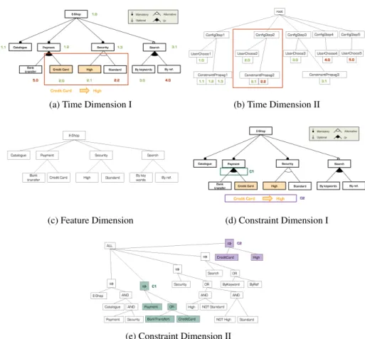
Based on these definitions, we have defined three dimensions and four measures which characterize a product configuration process. We illustrate them by taking a configuration process for the simple feature model E-Shop illustrated in Figure 1a. The numbers noted on the feature model correspond to the choices either explicitly made by a user (steps: 1.0, 2.0, 3.0, 4.0, 5.0), or propagated automatically by config-uration tool to satisfy constraints (steps: 1.1, 1.2, 1.3, 2.1, 2.2, 3.1). Figures 1a to 1e depict the elicited dimensions.
2.1.1. The dimensions
Time dimension. The configuration process can be seen as a succession of steps in a workflow [HUB 09], where each step relates to one or more choices. Thus, under-standing a configuration state requires consequently to analyse when a feature choice
(a) Time Dimension I (b) Time Dimension II
(c) Feature Dimension (d) Constraint Dimension I
(e) Constraint Dimension II
Figure 1. Feature Model Configuration Dimensions
has been made or propagated. Thus, we introduce the time dimension to describe this succession of steps. Each configuration step is composed by a stakeholder feature choice which may be automatically followed by a constraint propagation. Figure 1b, illustrates the time dimension for the E-Shop example. In this figure, the content of the red rectangle illustrates the organization of the configuration step two contained inside the red rectangle of Figure 1a. The configuration step two is composed by the sub-step Credit Card user choice (2.0) and by the sub-step propagation of constraints which causes the automatic selection of the feature High (2.1) and the automatic rejection of the feature Standard (2.2).
Feature dimension.As the goal of the configuration task is to decide which fea-tures will be included in or excluded from the final product, the feature concept is key to the configuration concept. Figure 1c shows the hierarchical organization of the feature dimension which is identical to the feature model structure.
Constraint dimension.The presence of constraints amongst features restrains the possible configuration choices. Resultantly, a stakeholder needs to know during his configuration task if a constraint is already resolved or not. The constraint dimension gathers two types of constraints defined in the feature model: the constraints between a parent feature node and its child feature nodes and the cross-tree constraints. In the constraint dimension, the representation of a constraint is an algebraic tree whose the leafs are logical literals involving a feature and the internal nodes are logical opera-tor. Figure 1e illustrates the hierarchical organization of the constraint dimension. In particular the colored parts C1 and C2 highlight the constraints representation respec-tively contained in the frames C1 and C2 of Figure 1d.
2.1.2. The measures
As introduced above, measures are defined with respect to one or more dimensions. Feature state. This categorical measure is defined regarding time and feature dimensions. Feature state is quite straightforward considering the configuration task: it aims at informing a feature state (selected, rejected or choice free).
Feature state origin.This categorical measure is defined on the time and feature dimensions and allows to ascertain if a feature state change is due to a stakeholder choice (chosen) or to a propagation of constraint (deduced). For example, in Figure 1a, the selection of the feature Credit Card (2.0) is chosen by a user and consequently the selection of the feature High (2.1) is deduced.
Constraint state. This categorical measure is defined on the time and constraint dimensions and allows to know if a constraint is resolved or not. For example, in Figure 1d, the constraint C2 is not resolved before the configuration step two and becomes resolved after this step.
Feature-constraint involvement.This categorical measure is defined on the fea-ture and constraint dimensions and allows to analyse if a link exists between a feafea-ture state and a constraint state. For example, in Figure 1e, the features Credit Card and High are involved in the constraint C2.
Our dataset is limited to simple configuration process, more sophisticated situa-tions will lead to the extension of this dataset by adding other measures.
2.2. Methodology
To create dedicated visualizations, it is necessary but not sufficient to characterize a generic dataset for the whole process, we need to precisely relate visualizations to user tasks and objectives within the configuration process. Here, we offer some methodological insights to do so.
2.2.1. Dataset restriction
The first step consists in choosing the most suitable dimensions, dimension mem-bers and measures relevant for a given task of the user within the configuration pro-cess, yielding a subset of the dataset. For example, finding at a given point in time t which choices have been made by a user and which choices have been automatically deduced from the propagation of constraints involves the feature dimension, only the member t of the time dimension and the measure feature state origin. Knowing in which constraints a given feature is involved does not need the time dimension. Ad-ditionally some measures can be derived from the subset thus defined. We will see an illustrative example of this kind of measure in section 3.
2.2.2. Visualization solution elicitation
We intend to find an adapted visualization for the data subset identified which con-tains some dimensions or part of dimensions and some measures. The characterization of the dimensions/measures in section 2.1 and the number of elements contained in the subset influences the selection of the visualization solution.
Proposing a complete visualization solution for the restricted dataset requires to consider a static view and to integrate some dynamic aspects allowing the user to understand the configuration process in a customized way.
In order to elaborate the static part, we have to define a visualization for all the subset elements defined in section 2.2.1.
A visualization can be a simple element like a shape, a color, a texture, an orientation [BER 83]. The visualization elements are classified depending on their perceptual qualities [MOO 09]. The choice of a particular visualization element must be related to the type of measure to visualize. For example, the visualization of a categorical measure requires the distinction between its different values. As a color variation is appropriate to highlight the difference between two elements [MOO 09], we can use color to encode the different values of a categorical measure. We must also take into account the number of different measures to visualize at the same time. Indeed, in the case of different measures, we can combine the visualization elements. For example, the visualization of a red rectangle combines a shape and a color elements and can thus represent two different measures.
A visualization can also be a particular visualization design (see for example the nu-merous representations of hierarchical data available in [SCH 11]). The choice of a particular visualization design is influenced by the number of dimensions involved in the subset and by the type of the dimensions. For example, the presence of the time dimension needs a visualization design adapted for the time-oriented data [AIG 08]. Moreover, the number of members contained in the dimensions (i.e the size of the di-mensions) have an impact on the visualization design as it determines the data quantity to display. Several space-filling visualization design exists [STA 00] which optimize the number of elements displayed on the space screen.
We consider now the dynamic part. We have to integrate interactive visualization techniques which offers the user to modify temporarily some chosen aspects of the proposed view. During the task management process, some data can be less important than the others. We need to identify this data in order to give the user temporarily the possibility to hide it or to make it less visible. The user can thus focus on the crucial data for his configuration task. To this purpose, several mechanisms [SPE 00] offer to display in detail or highlight the relevant information and to skip or overview less relevant information.
3. Example
We illustrate our approach on a specific configuration task issue: understanding the impacts of a feature selection or rejection. We are therefore in the following sit-uation: a stakeholder makes a new configuration choice. We intend to represent the consequences (propagations) of such a choice on the other feature states so that the stakeholder can better understand them. As an illustrative example, we have chosen the feature model of a Graph Product Line (GPL).
3.1. Subset definition
Showing the consequences of a given choice leads to presenting the feature model state before the choice and then the resulted changes on the feature states after this choice.
We will define firstly the dimensions and secondly the measures required to illus-trate the targeted problem.
As we need to present the feature model, the feature dimension is required in the subset. The time dimension is also involved since we have to present the state of the feature model at a given point in time t (before the choice) and at a given point in time
t + 1 (after the choice). We are only interested by the specific t and t + 1 members of
the time dimension.
Regarding measures, feature state, defined over time and feature dimensions is naturally the most relevant here and we need to know its values for each features at the given points in time t and t + 1. Additionally, we want to distinguish at the given point in time t + 1 the feature state change chosen by the user from the feature state changes which are the consequences of this choice. For this purpose, the measure
feature state origin defined as well over time and feature dimensions is interesting
at the given point in time t + 1. According with the definitions mentioned in 2.1, we select resultantly for each feature member, the fact containing the value of the measure feature state related to the t time dimension member and the fact containing the values of the measures feature state and feature state origin related to the t + 1 time dimension member.
Additionally, we have to catch the feature states changes between the given point in time t (before the choice) and t + 1(after the choice). For each feature member of the feature dimension, we compare the fact corresponding to the t time dimension member and the fact corresponding to the t + 1 time dimension member. We check if the feature state measure value has changed. Resultantly, we obtain a list of the feature states which have been modified between t and t + 1. This list is an illustrative example of a measure derived from the existing subset as mentioned in section 2.2.1.
Therefore, the subset contains the feature dimension, the members t and t + 1 of the time dimension, the feature state measure values for all the features at the point in time t, the values of the measures feature state and feature state origin for all the features at the point in time t + 1 and the deduced list of modified feature states. We need now to find a visualization solution for this subset in mapping the subset data to visualization elements.
3.2. The visualization solution
We explained in section 2.2.2 that the choice of the visualization solution depends on the type of dimensions/measures but also on the size of the dimensions. For this example, we focus on the type of dimensions/measures contained in the data subset and we do not consider the size of the dimensions.
We need to construct the visualization static part. To this purpose, we associate the subset of dimensions/members/measures with selected visualizations.
The presence of the time dimension in the subset is generally a major element to take into account for the choice of a visualization design [AIG 08]. The solution must indeed be able to represent the data evolution over time. In this example, as only two time dimension members are involved in the subset, the only data evolution to visualize is the difference of the feature state measure values between this two points in time.
For the subset elements, the mapping is thus the following:
The feature dimensionis essential for the feature model visualization. It has a hierarchical organization and resultantly we need a visualization design adapted for the hierarchical data. We choose a classical horizontal tree visualization design whose the feature nodes are represented with a circle and an affixed feature name text label. A feature state measure valueis categorical. We choose to represent a feature state with a color visualization element: the color of the feature node circle circumference (green for selected, blue for free and red for rejected). A feature state origin measure value is categorical. We choose to distinguish the only feature state chosen by the user at the given point in time t + 1. For this purpose, the name text label of the corresponding feature is in bold and in the color corresponding to the feature state whereas the other name text labels are not in bold and in black color. The feature state changes between the points in time t and t + 1 are important elements to visualize the impacts of a feature choice. As the color is particularly adapted to show the difference between
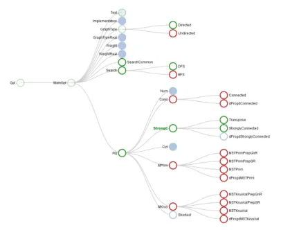
Figure 2. Derived Visualization
two elements [MOO 09], we choose to represent the feature state changes with a color visualization element. We keep the color code already used for the feature state but we modify the color transparency. We add transparency to the circle circumference color for the unmodified feature state changes whereas the circle circumference color for the feature state changes is opaque.
Concerning the dynamic part, we want to optimize the space screen and to focus the user attention on the changes. We add a visualization technique which by default, folds all the tree branches which do not contain a feature state change. We obtain a temporarily view where only the tree parts containing feature state changes are dis-played. Obviously the user can then unfold the branches as it sees fit. To that purpose, the user must know if, for a given node, there are folded children to unfold or if the node is a leaf. As we have only used the circle circumference color to represent the feature state, we can use the inner circle filling to indicate a children presence.
Figure 2, is a screenshot of our visualization solution, which we implemented using the D31javascript library.
Figure 3. FeatureIDE Visualisation
3.3. Comparison with an existing configuration tool
We want to compare our feature model configuration view in Figure 2 with the Feature IDE [THU 12] advanced configuration view in Figure 3 and with the S2T2 [PLE 12] configuration view. However S2T2 does not manage the complex cross-tree constraints implying more than two features. Our example contains this type of constraints, consequently it was not reproducible on S2T2 and we compare only our configuration view with the Feature IDE advanced configuration view.
The initial state of the feature model contains the selection of the features Gpl, MainGpl, GraphType, Test, StartHere and Base. A user select the feature StrongC and we aim at visualizing the twenty-three feature impacts due to this selection. The screenshots presented in Figure 2 and in Figure 3 show the configuration view after the choice of the feature StrongC. For the two screenshots the screen resolution used is 1280*1024 px and the configuration view space screen is 1000*842 px.
In Figure 2, as explained in section 3.2, only the tree branches containing the feature impacts are unfold by default. Resultantly, the whole feature model can be displayed on the space screen and the impacts are highlighted. The text label of the StrongC selected feature is in green and bold. Moreover, the feature selections which were already validated before the new StrongC feature selection appear in transparent green whereas the new StrongC feature and its impacts appear in opaque green (if the feature is selected) or in opaque red (if the feature is rejected). The feature state
StartHere and Base are folded under the node Test as these selections of features were accomplished before the new StrongC choice.
In Figure 3, we notice that the Feature IDE configuration tool unfolds by default all the branches of the feature model tree. Consequently, on the space screen, the whole feature model can not be displayed and in particular, the twenty-three impacts are not visible even if the screenshot focuses on the tree part with the maximum of visible impacts. The user can not visually identify his last feature state choice given that the StrongC feature is not distinguishable from the other features. Additionally, as the new choice and its impacts are not highlighted, a stakeholder can not make the distinction between the feature model state before the new StrongC feature selection and after.
We strongly believe that reasoning in terms of dimensions, measures and facts, helps us asking the right questions the visualizations should answer and avoid the pitfalls encountered above.
4. Conclusion
In this paper, we delineated a systematic approach to design cognitively-effective visualization solutions for configuring products in SPLE context. In particular, we ex-plained how to decompose configuration information in terms of an evolving dataset, defined basic dimensions and measures helping human understanding of the config-uration process and eliciting the most suitable visualizations. We illustrated our ap-proach by explaining how, from a configuration task issue example, we found a simple visualization solution adapted to the configuration data involved in this specific task issue. We are just defining the initial steps of our method and there is therefore room for future work. First, we would like to extend our dataset to take into account more expressive feature modelling constructs such as attributes and cardinalities, to visual-ize e.g. non-functional properties of configured products [SIE 13]. Second, we want to study the impact of quantitative measures on the derived visualizations.
5. References
[AIG 08] AIGNERW., MIKSCH S., MULLER W., SCHUMANNH., TOMINSKIC., “Visual methods for analyzing time-oriented data”, Visualization and Computer Graphics, IEEE
Transactions on, vol. 14, num. 1, 2008, p. 47–60, IEEE.
[AIG 11] AIGNERW., MIKSCH S., SCHUMANNH., TOMINSKIC., Visualization of
time-oriented data, Springer, 2011.
[BER 83] BERTINJ., Semiology of graphics: diagrams, networks, maps, University of Wis-consin press, 1983.
[CAR 99] CARDS. K., MACKINLAYJ. D., SHNEIDERMANB., Readings in information
[DEE 04] DEELSTRAS., SINNEMAM., BOSCHJ., “A product derivation framework for soft-ware product families”, Software Product-Family Engineering, p. 473–484, Springer,
2004.
[HUB 09] HUBAUXA., CLASSENA., HEYMANSP., “Formal modelling of feature configura-tion workflows”, MUTHIGD., MCGREGORJ. D., Eds., Software Product Lines, 13th
In-ternational Conference, SPLC 2009, San Francisco, California, USA, August 24-28, 2009, Proceedings, vol. 446 of ACM International Conference Proceeding Series, ACM, 2009,
p. 221–230.
[KAN 90] KANG K. C., COHEN S. G., HESS J. A., NOVAK W. E., PETERSON A. S., “Feature-oriented domain analysis (FODA) feasibility study”, report , 1990, DTIC Doc-ument.
[MOO 09] MOODYD., “The Physics of Notations: Toward a Scientific Basis for Constructing Visual Notations in Software Engineering”, Software Engineering, IEEE Transactions on, vol. 35, num. 6, 2009, p. 756-779.
[MUR 13] MURASHKINA., ANTKIEWICZM., RAYSIDED., CZARNECKIK., “Visualization and exploration of optimal variants in product line engineering”, Proceedings of the 17th
International Software Product Line Conference, ACM, 2013, p. 111–115.
[NÖH 10] NÖHRER A., EGYEDA., “C2O: a tool for guided decision-making”, Proceed-ings of the IEEE/ACM international conference on Automated software engineering, ACM,
2010, p. 363–364.
[PLE 12] PLEUSSA., BOTTERWECKG., “Visualization of variability and configuration op-tions”, International Journal on Software Tools for Technology Transfer, vol. 14, num. 5, 2012, p. 497–510, Springer.
[RAV 10] RAVATF., TESTEO., ZURFLUHG., “Algebre OLAP et langage graphique”, arXiv
preprint arXiv:1005.0213, , 2010.
[SCH 11] SCHULZH., “Treevis. net: A tree visualization reference”, Computer Graphics and
Applications, IEEE, vol. 31, num. 6, 2011, p. 11–15, IEEE.
[SHE 10] SHES., LOTUFOR., BERGERT., WASOWSKIA., CZARNECKIK., “The Variability Model of The Linux Kernel.”, VaMoS, vol. 10, 2010, p. 45–51.
[SIE 13] SIEGMUNDN., ROSENMÜLLERM., KÄSTNERC., GIARRUSSO P. G., APEL S., KOLESNIKOVS. S., “Scalable prediction of non-functional properties in software product lines: Footprint and memory consumption”, Information & Software Technology, vol. 55, num. 3, 2013, p. 491–507.
[SPE 00] SPENCER., PRESSA., Information visualization, Addison Wesley, 2000.
[STA 00] STASKOJ., CATRAMBONER., GUZDIALM., MCDONALDK., “An evaluation of space-filling information visualizations for depicting hierarchical structures”, International
Journal of Human-Computer Studies, vol. 53, num. 5, 2000, p. 663–694, Elsevier.
[STE 04] STEGERM., TISCHERC., BOSSB., MÜLLERA., PERTLERO., STOLZW., FER
-BERS., “Introducing pla at bosch gasoline systems: Experiences and practices”, Software
Product Lines, p. 34–50, Springer, 2004.
[TEL 08] TELEAA. C., Data visualization: principles and practice, Ak Peters, 2008. [THU 12] THUMT., KSTNERC., BENDUHNF., MEINICKEJ., SAAKEG., LEICHT.,
“Fea-tureIDE: An extensible framework for feature-oriented software development”, Science of