HAL Id: tel-00002076
https://tel.archives-ouvertes.fr/tel-00002076v2
Submitted on 3 Jan 2003
HAL is a multi-disciplinary open access archive for the deposit and dissemination of sci-entific research documents, whether they are pub-lished or not. The documents may come from teaching and research institutions in France or abroad, or from public or private research centers.
L’archive ouverte pluridisciplinaire HAL, est destinée au dépôt et à la diffusion de documents scientifiques de niveau recherche, publiés ou non, émanant des établissements d’enseignement et de recherche français ou étrangers, des laboratoires publics ou privés.
Options Réelles et Options Exotiques, une Approche
Probabiliste
Laurent Gauthier
To cite this version:
Laurent Gauthier. Options Réelles et Options Exotiques, une Approche Probabiliste. Mathématiques [math]. Université Panthéon-Sorbonne - Paris I, 2002. Français. �tel-00002076v2�
UNIVERSITE PARIS I PANTHEON-SORBONNE
U.F.R. M
ATHEMATIQUES ET
I
NFORMATIQUE
OPTIONS REELLES ET OPTIONS EXOTIQUES,
UNE APPROCHE PROBABILISTE
T
HESE
Pour le Doctorat de l'Université Paris I en Mathématiques
par
Laurent GAUTHIER
Presentée le 27 Novembre 2002
Directeurs de recherche :
M. Marc CHESNEY, Professeur à HEC
M. Elyes JOUINI, Professeur à l'Université Paris IX et à l'ENSAE
Membres du Jury :
Mme. Monique JEANBLANC-PICQUE, Professeur à l'Université d'Evry, rapporteur
M. François QUITTARD-PINON, Professeur à l'Université Lyon I, rapporteur
M. Nizar TOUZI, Professeur à l’Université Paris I
M. Marc YOR, Professeur à l'Université Paris VI
Cette thèse a été entamée en 1996 et sa rédaction s’est étalée sur environ cinq ans: 2 ans
d’écriture, et 3 ans relecture et corrections. Je tiens à remercier mon directeur de thèse Marc
Chesney qui, tout ce temps, m’a encadré et aiguilloné. C’est grâce à son intérêt pour les options
réelles que j’ai pu découvrir ce domaine depuis 1994. Marc Chesney m’a très judicieusement
conseillé, soutenu et aidé ; je lui en suis très reconnaissant.
J’ai beaucoup apprécié qu’Elyès Jouini accepte de co-diriger ma thèse et m’accueille à la
Sorbonne en 1997, après que j’ai suivi quelques cours du DEA de Modélisation Mathématique
de Paris-I. Elyès Jouini m’a inspiré dans mon approche des coûts de transaction, et je lui suis
aussi reconnaissant de m’avoir aidé à orienter mes recherches, tout en me laissant une grande
liberté.
Je tiens à remercier très chaleureusement Monique Jeanblanc-Picqué et François Quittard-Pinon,
mes rapporteurs. Monique Jeanblanc-Picqué a décortiqué cette thèse, et sans elle de nombreux
résultats dans ce travail seraient soit faux, soit démontrés de manière un peu trop heuristique.
Parmi mes agréables souvenirs d’étudiant, le cours de calcul stochastique de Monique
Jeanblanc-Picqué au doctorat HEC occupe une place particulière.
François Quittard-Pinon a accepté d’être un rapporteur, et je lui sais gré de son temps. J’espère
sincèrement que cette lecture l’a intéressé et en valait la peine.
Je remercie également Marc Yor de faire partie de mon jury de thèse. Je le remercie aussi et
surtout pour l'enseignement qu'il m'a dispensé en DEA. C’est à lui que je dois mes quelques
connaissances sur l’étude fine du mouvement brownien.
Nizar Touzi a eu la gentillesse d’accepter de participer à mon jury de thèse, et je lui en suis
reconnaissant. Les aspects mathématiques et les applications financières de cette recherche, je
l’espère, l’intéresseront.
Je n’oublie pas Erwan Morellec, mon collègue doctorant et co-auteur, avec qui j’ai toujours eu
des discussions intéressantes et fructueuses.
Finalement, les arbitres des revues auxquelles j’ai soumis differente parties de cette thèse ont
réellement contribué à la qualité de mon travail, en relevant de nombreuses erreurs ou bien tout
simplement en remettant en question ma première approche.
OPTIONS REELLES ET OPTIONS EXOTIQUES, UNE APPROCHE PROBABILISTE
Cet ouvrage se concentre sur la valorisation et la couverture d'options financières non traitées sur les marchés, les options réelles, qui servent à évaluer des décisions optimales d'investissement en capital pour des entreprises. L'existence pour une entreprise d'un projet d'investissement s'apparente en effet à la possession d'une option financière: l'entreprise possède l'option d'attendre le moment le plus favorable pour lancer son projet. Pour valoriser l'intérêt économique d'un projet, il convient alors de calculer la valeur de l'option d'investir. L'objectif de cette thèse est de montrer comment la théorie des options réelles peut bénéficier des apports des méthodes habituellement employées pour les options exotiques.A la différence de l'approche classique dans le domaine des options réelles, qui privilégie l'utilisation de techniques d'équations différentielles, nous proposons dans cette thèse d'évaluer des projets d'investissement en applicant des méthodes très probabilistes. Cette distinction de méthode permet non seulement de généraliser l'approche classique du problème, mais encore d'obtenir des résultats analytiques dans des situations ou une technique d'équation différentielle ne permettrait pas de résoudre le problème. Egalement, c'est un pont jeté entre la recherche académique en finance d'entreprise et la floraison de nouveaux résultats sur les options exotiques, très souvent obtenus par des approches probabilistes.
Dans cette thèse, nous abordons spécifiquement des problèmes
•= de valorisation de projets d'investissement sous certaines contraintes particulières : lorsqu'il existe un délai incompressible entre la prise de décision et sa mise en oeuvre, lorsqu'il existe une compétition entre deux acteurs économiques de caractéristiques différentes, et lorsque l'information sur le marché de l'entreprise est imparfaite.
•= de couverture de ces projets d'investissement : comment couvrir des options réelles qui sont un peu complexes de la manière la plus efficace lorsqu'il existe des coûts de transaction sur les actifs financiers, et comment une nouvelle classe de produits dérivés qui s'apparentent aux options barrières permet de couvrir le risque lié à l'exercice des options réelles.
•= de décision optimale d'investissement lorsque l'on peut manipuler le marché : un agent économique qui possède une information privilégiée sur la valeur d'une entreprise peut intervenir sur le marché afin de l'utiliser, et par la même occasion influencer la valeur des titres émis par l'entreprise. Quelle est sa stratégie optimale ?
Les outils mathématiques utilisés sont surtout probabilistes, essentiellement la théorie des excursions, les temps locaux et le contrôle stochastique. Le principal souci est l'obtention de résultats analytiques, au détriment du développement de méthodes numériques.
This work focuses on valuing and hedging financial options that are not traded, called real options, and that are used to assess corporations' optimal capital investment decisions. For a company, the existence of an investment project is similar to owning a financial option: the company possesses the option to wait for the most favorable time to launch its project. Assessing the economic attractiveness of a project therefore requires to value this option. Our objective is to show how real option theory can benefit from exotic options methods.
Unlike the classical approach in real options, which favors using differential equations techniques, we propose to value investment projects with probabilistic methods. This distinction allows not only to generalize the approach, but also to obtain analytical results in cases when a differential equation approach would not prove tractable. Also, it relates a corporate finance research domain with the very flourishing field of exotic options, a field where most results are obtained through probabilistic tools.
Specifically, we tackle
•= the valuation of investment projects when there is a delay between the decision to invest and its actual implementation, when there is a competition between two economic agents with different delay-related constraints, and when the information available to the firm is noisy,
•= the hedging of investment projects: how to hedge real options in the most efficient manner when there are transaction costs on the underlying assets, and how a new class of derivatives products that are related to barrier options allow to hedge the risk related to exercising real options
•= the optimal investment decision of an agent who has an impact on the market. An economic agent possessing privileged information on a company can trade its stock with profit, while pushing the market price towards the price that reflects the information. What is the agent's optimal strategy?
The mathematical tools used are essentially probability, the theory of excursions, local times, and stochastic control. We are especially interested in obtaining analytical results, rather than in finer modeling or developing numerical methods.
Contents
1 Introduction 11
2 Decision Delays and Embedded Options1 17
The traditional approach . . . 19
General model of delayed investment decisions . . . 20
Implementation delay and embedded options . . . 23
Implementation delay with no exit option: . . . 23
European abandonment option . . . 25
The Parisian abandonment option . . . 26
American abandonment option with an exponential exercise barrier 30 Concluding remarks . . . 32
References . . . 33
3 The Mathematics of Delayed Investment Decision2 35 A simple and interesting stopping time . . . 35
Computation of the first instant where d units of time after having hit a level, the Brownian Motion is above another level . . . 35
Laplace transforms for a drifted Brownian motion . . . 39
Computation of the first instant when the Brownian Motion spends more than d units of time over a non-constant barrier, while having to go back to zero . . . 40
Laplace transforms for the drifted Brownian motion . . . 42
The Parisian stopping time . . . 43
The Laplace transform of the first time a positive Brownian excur-sion reaches a certain length . . . 43
A second proof of Chesney, Jeanblanc, Yor’s theorem . . . 45
Excursion theory related stopping times . . . 47
Reformulation of the integral . . . 47
A useful path decomposition based on the balayage principle . . . 48
Computations of the path integral related to the longest excursion 48 A third proof of Chesney, Jeanblanc, and Yor’s theorem . . . 50
References . . . 51
1The original version of this chapter was co-written with Erwan Morellec and is to appear in Real Options and Investment under Uncertainty, Eds. E. Schwartz and L. Trigeorgis, MIT Press.
2
The part of this chapter that focuses on the alternative proofs of the Theorem of Chesney, Jeanblanc and Yor is to appear in the Advances in Applied Probability, under the title ”Parisian Options: A Simplified Approach without Excursions”
4 Decision Delays in Asymetric Dual Competition3 53
The model . . . 54
Investment decision and options . . . 55
Competition between a large and a small companies . . . 56
The up and out Parisian call . . . 56
The case of an already started excursion . . . 59
On the length and height of excursions . . . 60
Exploiting the links between the three expressions . . . 61
Reformulation of Ehe−ρHD+∧Ta i . . . 64
Explicit computation of Itô measure integrals . . . 67
Expression of the desired quantities . . . 72
The large company’s strategic behavior . . . 72
If both firms have full information . . . 73
If the big firm has limited information . . . 74
Concluding remarks . . . 75
References . . . 76
An application to delayed investment decision . . . 77
5 Noisy Information and Investment Decision4 79 The model . . . 80
The noisy model . . . 80
Optimal investment decisions with noisy uncertainty . . . 81
Noisy information and real options values . . . 83
Concluding remarks . . . 84
References . . . 85
6 Hedging Real Options with Transaction Costs: a Convergence Result5 87 The model . . . 89
Derivatives redundant hedging . . . 89
Leland’s hedging strategy . . . 93
The risk-related hedging strategy . . . 96
The path-dependent case with transaction costs . . . 99
Proof of the convergence results . . . 100
Applications to options pricing . . . 108
Existence of solutions to the pricing equations . . . 109
Approximating the solution of the non-linear PDE . . . 111
Reducing the set of possible replication strategies . . . 112
Concluding remarks . . . 113
References . . . 113
Appendix: the path-dependent case . . . 114
3A different version of this chapter has also been co-written with Marc Chesney, using a more analytical approach. The technical part of this chapter that focuses on the lenth and height of excursions is to appear in the Journal of Applied Probability in December 2002, under the title ”Excursion Length and Height and Application to Finance”.
4A version of this chapter, co-written with Erwan Morellec, has been published under the title ”Noisy Information and Investment Decision: a Note”, Finance (PUF) 1999, 20(2).
5
A shorter version of this chapter has been published under the title ”A Transaction Cost Convergence Result for General Hedging Strategies” in Stochastic Models (Dekker), 17(3), pp. 313-339 (2001).
7 Hedging Entry and Exit Decisions6 119
Real options: entry and exit decisions . . . 120
The pricing of switch options . . . 124
Relationship between Switch options and real options. . . 129
Switch options as a replication tool . . . 129
Switch options to hedge entry and exit costs . . . 129
The joint law of the Brownian meander and its running supremum . . . 131
Concluding remarks . . . 132
References . . . 132
8 Manager’s Opportunistic Trading7 133 A model for the market impact of transactions . . . 134
Infinite market size model . . . 135
Remarks on the infinite size market model . . . 137
The case of a market with a limited number of assets . . . 140
Some remarks on the limited size market model . . . 141
Controlling the BM in a tunnel . . . 142
The law of the controlled Brownian Motion . . . 142
Distribution of the cost of control . . . 145
Market manipulations and arbitrage . . . 146
The setting of the model . . . 146
The value of a strategy in the infinite market model . . . 147
The value of the strategy in the finite-size market . . . 150
Imperfect information . . . 151
The optimal strategy . . . 152
The impact of informed trading on the evolution of prices . . . 155
Concluding remarks . . . 157
References . . . 157
Appendix . . . 159
Platen and Schweizer Theorem . . . 159
The case of a singular control . . . 159
9 Conclusion 163
6This chapter has been published in the Journal of Applied Mathematics and Decision Sciences (Erlbaum), 6(1), pp. 51-70 (2002), under the title ”Hedging Entry and Exit Decisions: Activating and Deactivating Barrier Options”.
7A shorter version of this chapter is to appear in the International Journal of Applied and Theoretical Finance under the title ”Informed Opportunistic Trading and Price Optimal Control”.
List of Tables
2.1 Valuation of the European Entry Option . . . 27
2.2 Valuation of the Parisian Entry Option . . . 29
5.1 Effect of Noise on Valuation . . . 83
5.2 Combined Effect of Noise and Volatility . . . 84
7.1 Valuation of an Active Project . . . 124
7.2 Valuation of an Inactive Project . . . 124
8.1 Value of Manipulation vs. Maximal Trade Size . . . 154
8.2 Influence of v on Manipulation Value . . . 154
List of Figures
1 Implementation Delay and no Exit Option . . . 24 2 Implementation Delay with European Exit Option . . . 26 3 Implementation Delay with Parisian Option . . . 27 4 Implementation Delay with Exponential Exercise of the Exit Option 31
Chapter 1 INTRODUCTION
The study of probability has been historically linked to decision problems. Pascal’s motivation in 1654 when he wrote his ”Adresse à l’Académie Parisienne” was to assess the fairest repartition of the bets if a random game was interrupted. Probability at its birth was closely associated with financial and economic issues. In 1900 Bachelier in his ”Théorie de la Spéculation” provided a basis for Markovian diffusion processes, that were to be rediscovered in 1933 by Kolmogorov. Finally, Black, Merton and Scholes published in 1973 a series of fundamental papers where they valued financial products by calculating the expectation of a function of a Brownian Motion.
Since then, financial mathematics have become a flourishing branch of proba-bility and mathematical analysis. Black, Merton and Scholes’s result allowed for the development of new financial markets, inducing a significant need for research in this field. Throughout the past 25 years, considerable resources were allocated to adapting original models to new problems. It clearly appears that a symbiotic evolution took place: markets develop and mature thanks in part to new models and technical paradigms, which pushes financiers towards innovating and creating new markets so that they can maintain profitability in the business, and these new markets require new models.
A large majority of mathematical finance research has been carried out in the field of financial derivatives. These products give their owners future income streams that are a function (specified in advance) of other products’ value. These other financial products are called the underlying of the derivative. From a math-ematical perspective, the value of an underlying is modeled as a diffusion process, and the value of the derivative is often the expectation, under a certain probability, of a functional of this underlying process. Since 1973, the thorough study of the Brownian Motion has allowed the valuation of more and more complex derivatives, such as ”barrier options” that are related to hitting times, or ”mean options” re-lated to exponential integrals of the Brownian Motion. Besides, accounting for realistic market-related constraints required the intensive use of stochastic con-trol, in particular of the notions of viscosity solution or optimal stopping. Market ”non-completion” problems (the fact there always exist a risk against which one cannot be insured) have induced significant research on the existence of equivalent probabilities, or on projections onto semi-martingale spaces.
Financial derivatives, which are traded on many markets with extremely high volumes, can also be used to model micro-economic decisions. There is a simple analogy: a company that wishes to invest in a project possesses the option to wait for better conditions to implement this investment. This option is in fact very much like a financial derivative, and its underlying consists of the economic variables that will condition the future value of the project (such as the market share, the value of the products sold or bought or the intensity of demand). This option is a so-called ”real option” and its valuation is similar to that of financial derivatives. The theory of real options was developed through the 1980s, benefiting from the wide success of financial derivatives. Real options have been mentioned in Business Week1. For managers, real options appear as superior to the traditional
method of discounting future cash flows so as to decide whether to invest or not.
1Coy, Peter, ”Exploiting Uncertainty: The ’Real Options’ Revolution in Decision-Making,” Business Week, June 7, 1999, pp. 118-124.
As written in Business Week,
”[By] boiling down all the possibilities for the future into a single sce-nario, NPV [Net Present Value] doesn’t account for the ability of ex-ecutives to react to new circumstances - for instance, spend a little up front, see how things develop, then either cancel or go full speed ahead”
However, as much as the field of probability benefited from the new problems posed by financial derivatives, the mathematical methods used to study real op-tions were not demanding in terms of mathematical research. Real opop-tions being from the start more related to corporate finance than market finance, most of the research in their field has been performed on a more economic tradition. From a technical perspective, it translates into a generalized use of differential equations, rather than pure probabilistic tools. This work focuses on the frontier between ex-otic options and the probabilistic methods associated to them on one side, and real options on the other side. Unlike financial derivatives that are traded on various markets, there is no limit to the complexity with which the decision to invest, or the constraints under which this decision is made, can be modeled. Approaching the problem from a probabilistic angle allows a greater freedom in modeling these constraints, as we will see.
Our goal is to show how the analysis of real options can benefit from con-cepts and methods that are usually employed for exotic options-related problems. So as to exploit the relationships between real options, probability, and exotic options, we will articulate our work as follows. The first part of this thesis fo-cuses on the valuation of investment projects under different constraints by the use of mathematical techniques usually applied to exotic derivatives. This part comprises Chapters 2 through 5. The second part focuses on the hedging of the risks related to investment decisions using financial options-related methods, and comprises Chapters 6 to 8.
The second chapter introduces the technical aspects of basic real option analy-sis from a probabilistic perspective. Then we proceed and study the effect, on the value of an investment project, of the delay existing between the decision to invest and its actual implementation. Numerous investment decisions are charac-terized by significant implementation delays. These delays can be linked to the search for an investment project, to the length of the decision process itself within the company, or to the time necessary to gather funding. We show that these implementation delays have an important impact on optimal investment decision rules as well as on the investment projects value. We show in particular that this loss of value can become negligible if the firm has the possibility to abandon the project during its implementation. From a technical perspective, we calculate the generating function of several stopping times related to the Brownian Motion. For example, we need to consider the first instant when a Brownian Motion spends continuously more than a given amount of time (the delay) above a barrier (the threshold that triggers the investment decision). We derive the value of this option for various exercise policies corresponding to different levels of freedom with re-spect to the abandonment of the project and analyze its effects on the investment policy of the firm. The mathematical results used in this Chapter are not new, but our application to real options and delay modeling had not been derived before.
The third chapter discusses the mathematical methods that can be used to study delay-related investment decision constraints. The probabilistic approach
we propose allows an unequaled flexibility in specifying the various constraints faced by investing firms or managers. Some results, as we will see, cannot be reached using conventional analytical approaches. This chapter presents no fun-damentally new mathematical result, but proposes a varied range of approaches to the computations involved by stopping times related the Brownian Motion and its excursions. Using mainly excursion theory, we show how to derive the generating function of some stopping times related to the modeling of delays in investment decisions. We show several proofs of the main result we used in Chapter 2 on the first instant the Brownian Motion spends consecutive time above a barrier.
The fourth chapter focuses on the competition situation between two firms interested in the same investment project, when they have different kind of con-straints. The real option approach fits very well the monopolist case. However, in a competitive case, the strategic behaviors of different firms is more complex to account for. Some authors have already tackled this problem and studied the preemption of investment projects in a real option framework. The aim of this chapter is also to consider this question, but in the case where the competitors have different constraints in terms of investment delay and flexibility: one firm is large, the other is small. In our setting, the large firm suffers a delay in its investment decisions, whereas the smaller firm’s decisions are instantaneously im-plemented. Calculating the value of the investment project, depending on the level of information available to each firm on its competitor, requires to study the first instant when a Brownian Motion spends more than a given amount of time above a certain level (that would model one firm’s investment, accounting for delay) or hits another higher level (that would represent the other firm’s decision). We de-rive the generating function of this stopping time and of other functionals by using excursion theory. To our knowledge, this result is new.
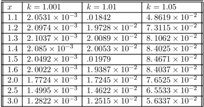
The fifth chapter studies the investment decision when the information on the underlying project is ”noisy”. When we look at empirical evidence, the option premium detected in those models seems to have a great statistical significance. However, most tests find that the option premium generated by the data is gen-erally spread over and under the value generated by the models. In competitive markets the winner’s curse can account for the undervaluation of the real option models. Another reason for this undervaluation may be that many models de-veloped so far are very simple and do not account for the investment projects ’embedded options such as the option to expand the investment size or the option to abandon the project. We show in this paper that the noise in the informa-tion available to the investor can account for their overvaluainforma-tion. The revenues associated with the exploitation of petroleum leases or mines is typically noisy as the extraction rate or the amount of reserves are subject to large forecasting errors. This chapter examines the effects of noise on investment decisions. We use the computation of first passage times to derive closed-form formulas relating the value of the investment opportunity to the noisy decision variable. Our setting for the description of the noise is simple but brings out the generality of the idea. We show that the value of real options, when we account for the noise, is lower than the option value computed in the perfect forecast case. For reasonable parameter values, our model can generate values for the investment opportunities very close to that observed in reality.
The sixth chapter considers the hedging of derivatives, whether they are fi-nancial derivatives or real options, using other fifi-nancial derivatives. As there are transaction costs, there is a balance between the frequency of transactions and
the quality of a financial product as a good hedge. For many firms, especially in the mining, oil, or commodities industries, the value of investment projects can be determined with real option theory. In these cases, an important argument underlying the valuation of projects is that the business risk, being linked to a traded product, can be hedged. Real options in that case can be considered as equivalent to complex options written on a commodity. In this paper, we address the issue of hedging such options, and more generally hedging complex options, using an optimal combination of underlying product and other derivatives written on it. The optimal hedging basket should minimize transaction costs, which can be important for derivatives, as well as for the underlying. There is a trade-off between hedging with a derivative that replicates locally well the real option but with a high transaction cost, or with the underlying at a lower transaction cost but a higher frequency of rehedging. This chapter generalizes the result of Leland (1985) to hedging strategies that use not only the underlying but all kinds of op-tions. These hedging strategies are a generalization of static hedging. In addition, the result is valid for all shapes of payoff, including path-dependent. Two cases of hedging methods are studied. The first one, as in Leland, assumes rehedging takes place at fixed time intervals. The second one supposes rehedging takes place when the delta moves by more than a fixed proportion. The pricing of securities in that frame can be done by solving a non-linear partial differential equation, and optimal hedging strategies, using various kinds of options, can be found so as to minimize transaction costs. The convergence result for the replication strategy is shown in detail.
The seventh chapter introduces a new sort of financial derivatives, which we christen ”switch options”. These products can hedge the risk related to the acqui-sition or to the business risk of an investment project. We define Switch options as path-dependent derivatives written on a single underlying that are activated every time the underlying hits a barrier and deactivated every time it hits another barrier. At maturity, if the option is activated, the holder receives a payoff that is a function of the underlying at that time; if it is not activated, the payoff is a different and lower function of the underlying’s price. The number of times such an option can be activated and deactivated is not bounded. Unlike a standard barrier option, the Switch option is never totally cancelled when the underlying hits the barrier, as there is always a chance it will go back and hit the other bar-rier. In this chapter we will first focus on the relationship between real options and Switch options. We also price these options and compare them with standard barrier options. The technical analysis makes use of the Brownian Meander, and in particular we derive the joint law of the Brownian Meander and its maximum. The eighth chapter focuses on the behavior of an informed investor. In this chapter we address the issue of quantifying the incentive to invest or disinvest from an equity investment to benefit from discrepancies between its real value and its market price. There exists an ”insider option” for informed agents: the option to arbitrage the market price based on privileged information about the firm’s projects. The decision of when to invest or disinvest and how much is indeed a real option based on market conditions. The exercise of such an option entails an effect on market prices. In this chapter we study the optimal arbitrage transactions an informed agent carries out and their influence on the market price. We model the discrepancy between the market price and the real value, known to the informed agent (maybe with some noise), and the impact on the market price of the trading strategy that maximizes the agent’s wealth. The effect of a
transaction on the price of a security determines how much it costs to trade this security, as well as the evolution of this price, which conditions future trading gains. We focus on the particular case of a manager trading his company’s own stock. An existing models for the impact of transactions on prices is extended to the case of discrete transactions. It is derived from simple assumptions on the behaviour of market participants. A probabilistic approach is proposed to determine the optimal control applied to the market price by the informed agent. Analytical solutions are derived to calculate the value of ”realigning the price” for an informed market participant, and the properties of the controlled market price are discussed.
Chapter 2 DECISION DELAYS AND
EMBEDDED OPTIONS
1
Since the early 80’s, advances in the real options literature have completely changed the way we evaluate investment opportunities. As shown in this literature, firms should not invest in projects which are expected to earn only the opportunity cost of capital. Managers can make choices about the project’s characteristics and this flexibility creates embedded options. These options add value to the project and invalidate the traditional net present value (NPV) rule. Among them, we can quote the option to defer the investment spending (McDonald and Siegel (1986)), the option to abandon an active project (Majd and Myers (1990)), the option to expand or to reduce the production capacity (Abel and Eberly (1996)) or the option to choose the production technology (He and Pindyck (1992)).
Although this literature has made a great step toward a better understand-ing of investment decisions, little research has focused on the practical side of the investment spending. One of the major characteristics of the capital budgeting process is the delay existing between the investment decision and its implementa-tion. This implementation delay is generally associated with the decision process within the firm or the gathering of the financing funds necessary to undertake the investment spending. Harris and Raviv (1996), citing Taggart (1987), assert that projects are generally initiated from the bottom up, suggesting a centralization of the capital allocation process. Depending on the nature and the size of the investment, projects that have been approved at the division level may have to be submitted to headquarters. Although all these intermediary steps take time, this point has been ignored without exception in the real options literature whereas it can have important consequences. Depending on the evolution of the decision variable during this implementation lag, the investment opportunity may have lost part of its attractiveness.
Beyond the analysis of the effects of capital budgeting practices within firms, typical applications of our model include the services offered by specialized invest-ment funds or the cost of the recourse to outside financing. For large projects it often takes considerable time to gather all the financing funds as the decision process within the institutions involved can be highly time consuming. For ex-ample, the time necessary to gather investors for a closed-end investment fund typically reaches one year during which the economic and market conditions can completely change. The type of financing funds may have an impact over the investment policy of firms as they condition the availability of the option to aban-don investment opportunities during the implementation delay. The use of outside funds, which typically destroys such options for reputation concerns in a classic manager-investor conflict as described in Jensen and Meckling (1976), reduces the value of the investment opportunity. There is nevertheless room for negotiation: if funds are raised externally the firm can pay the right to cancel the investment process, depending on the evolution of the decision variable. In the same way, the services offered by specialized investment funds constitute a typical application of these options. Investment opportunities on emerging markets can take time to be
1
THE ORIGINAL VERSION OF THIS CHAPTER WAS CO-WRITTEN WITH ERWAN MORELLEC AND IS TO APPEAR IN REAL OPTIONS AND INVESTMENT UNDER UN-CERTAINTY, EDS. E. SCHWARTZ AND L. TRIGEORGIS, MIT PRESS.
realized and an investment specialist can reduce the delay between the investment decision and its real implementation by providing a dedicated vehicle. The best example in that case is an open-ended fund. The price to pay for the immediacy of the opportunity is reflected in the bid-ask spread for the fund as opposed to a closed-end investment which prevents the early withdrawal of funds.
This paper analyses in a single unifying framework the valuation and behavioral consequences of the real options’ implementation delay. We use the computation of first passage times2 to derive closed-form formulas relating the value of the in-vestment opportunity and the inin-vestment threshold to the size of the delay. We find that the implementation delay can reduce the value of the investment oppor-tunity by a large amount when there are no ”minimum profitability requirements” once the investment decision has been taken. This result shows that the delay creates by itself the embedded option to abandon the investment project during its implementation should the decision variable evolve unfavorably. If the option is readily available, its value equals the increase in expected payoffs it permits. When the availability of this option depends on outside parties, its value consti-tutes the maximum price at which the agent holding the investment opportunity will be willing to negotiate it.
Using this general valuation framework, we compute the value of this option under alternative exercise policies corresponding to different minimum profitabil-ity requirements during the implementation period. We show that profitabilprofitabil-ity requirements generate a higher project value only if they apply to the whole im-plementation lag. Minimum profitability requirements at the imim-plementation date do not increase the welfare of investors when the investment decision is taken op-timally. Therefore, it is not optimal for the headquarters of a firm to force the operational division to invest only if the decision variable is above a new cutoff level at the end of the implementation delay. In the same way, there is no interest for the investing firm to negotiate with its partners a covenant allowing for its withdrawal from the project when all the financing funds are gathered. On the contrary we find that ”American” abandonment options increase the value of the investment project. Considering the difficulty of writing and enforcing contracts, we derive a so called ”Parisian3” abandonment rule that can be implemented at a low writing cost on the contrary to the value maximizing abandonment rule.
In the following section, we review the traditional approach where there is no implementation delay and the value of an investment opportunity is the solution to a free boundary problem similar to that of an American financial option. In section two, we use a general valuation framework to describe the effects of the implementation delay on investment decisions. Section three provides the optimal value of the investment opportunity under various abandonment policies associated with this implementation delay. Section four concludes the paper and presents possible extensions.
2
First passage times have already been used in the paper by Mauer and Ott (1995) in order to compute the mean replacement time of corporate assets. To our knowledge, our paper is the first that makes a systematic use of them. This singularity is due to the difficulty associated with the resolution of highly non linear ODE.
3See Chapter 3 and/or Chesney, Jeanblanc and Yor (1997) for a detailed presentation of Parisian options.
The traditional approach
We study the investment decision of a firm in a stochastic environment. At any time t the firm can invest in a project yielding an operating profit that depends on a decision variable (St, t ≥ 0) ruled by the diffusion process
½
dSt= St(µdt + σdZt)
S0= x
(2.1)
where µ and σ are constant and (Zt, t ≥ 0) is a Brownian motion defined on a
filtered probability space ³
Ω, F, (Ft)t≥0, P
´
4
. Ftrepresents the information
avail-able at time t.
The literature on real options describes the investment decisions of firm thanks to two technics closely related to each other: dynamic programming and contin-gent claims analysis. These technics essentially differ about the assumptions they involve concerning investors, the financial markets and the discount rates used by investors. Due to these differences, the results they yield are similar although not identical5.
One common characteristic of these models is the implicit assumption that actions are taken instantaneously: the project is started as soon as the investor has decided to invest. Using the stationary property and the Markovian property of the cash flows generated by the project, traditional real options models consider that the investment starts as soon as the decision variable (St, t ≥ 0) hits some
constant optimal level6.
The first valuation method used in the real options literature amounts to find-ing the optimization program of an investor through dynamic programmfind-ing argu-ments. This investor is generally risk neutral and has rational expectations. He maximizes the present value of the cash flow generated by the investment through an appropriate timing of the investment decision. Let us denote V (St, t) the value
of the investment project, f (St, t) the bounded monotonic profit flow function,
c+ (respectively c−) the investment cost for a positive (respectively negative)
in-vestment, and ρ the investor’s required rate of return i.e. the opportunity cost of capital7. The maximization program of this investor over an infinite time horizon can be written V (x, t) = max {h∗,l∗}E ½Z +∞ 0 e−ρs¡f¡Ssx,t, s¢ds − c+dPt+s+ c−dNt+s ¢¾ where Pt (Nt) is a non-decreasing (non-decreasing) function of time representing
the cumulation of positive (negative) investment spending up to time t, and (h∗, l∗) is the pair of values of the underlying variable corresponding to optimal investment decisions. The Bellman equation associated with this optimization problem in the continuation region is8
1
dtE [dV (St, t)] + f (St, t) = ρV (St, t) for St∈ ]l
∗, h∗[ (2.2)
4
(Ft, t ≥ 0) is the filtration generated by the Brownian motion 5
See Harchaoui and Lasserre (1995).
6Dixit and Pyndick (1994) provide a detailed presentation of this principle. 7
If the investor discounts all its future cash flows at a constant rate ρ then we must have ρ > µ for the expected present value of the payoffs generated by the project, E©Rt∞exp (−ρ (u − t)) Sudu/Ft
ª
, to be finite at any time t, t ≥ 0 when f is the identity. 8
subject to familiar value-matching and smooth-pasting conditions9 at S = h∗ and
S = l∗. The LHS of this equation is the expected return on the investment project whereas the RHS is the investor’s required return. The solution of this equation yields the optimal investment thresholds h∗and l∗and the value of the investment
opportunity.
The other valuation method relies on an analogy between real and financial investment decisions. The firm has an option to invest in a project and the value of this option can be found thanks to the usual contingent claim valuation framework. By an application of Theorem 3 of Cox, Ingersoll and Ross (1985), the value of the investment opportunity satisfies the following fundamental valuation equation
rV (St, t) =
1
2dtVSS(St, t) d hS, Sit+ 1
dtVS(St, t) (E [dSt] − λ (St, t) dt) + f (St, t) where r is the continuously compound risk-free interest rate and E [dSt] − λ (St, t)
is the risk adjusted 10 drift of the underlying variable (St, t ≥ 0). In order to find
λ (St, t) capital markets must be complete: there must exist an asset or a dynamic
portfolio of assets spanning the stochastic changes in the value function V (St, t).
The solution of this equation11 gives the value of the investment opportunity and the optimal exercise boundary of this option 12. Note that if the investment is perpetual and if f is independent of time, then the value function does not depend on time. In this case, the partial differential equation above becomes an ordinary differential equation.
General model of delayed investment decisions
In this subsection, we build a general valuation framework for the value of the investment opportunity when there is a delay between the investment decision and its implementation. Our analysis significantly differs from the ”time to build”13 literature as our implementation delay accounts for the lag existing between the decision to invest and the spending of the first dollar by the firm, not for the speed at which production facilities can be built.
As mentioned earlier, the implementation delay can be due to the research of an investment opportunity on an emerging market, to the capital budgeting process within the firm or to the time spent gathering the financing funds. Although our model applies to a wide range of implementation delays, we will emphasize in the following section the role of the capital budgeting process in altering the value of the investment opportunity. In order to keep the presentation simple, we will take the simplest environment possible. As in Harris and Raviv (1996), our firm is composed of headquarters and a single division14. The investment decision is initiated by the division manager but he must obtain capital from the
9
When the optimization program is strictly concave, i.e. when the indirect expected discounted payoff V (., .) is strictly concave, the boundary conditions ensuring that we are along the optimal path are called high-contact conditions and involve second order derivatives. See Dumas (1991) for a good exposition of value-matching, smooth-pasting and high-contact conditions.
1 0λ (S
t, .)is the risk premium associated with (St, t ≥ 0). 1 1
The boundary conditions used to solve this equation are the same than those used to solve equation (2).
1 2
When investment is reversible there are two exercise boundaries, one for investment and one for disinvestment.
1 3
In this literature each dollar invested in the investment opportunity gives the firm the option to spend another dollar in the project. See for example Majd and Pindyck (1987).
1 4Considering that the implementation delay reduces the value of the investment opportunity, the division would probably do better of as a stand alone entity. We do not address this issue
headquarters. This decentralization of the investment decision is due to the specific human capital of the division manager. We assume that he has no incentive to misrepresent his information but that the information transfer within the firm and the decisions concerning the capital allocation take time. We will focus on discretionary investments for which there is generally such a bottom up process.
In our setting agents are risk neutral and the firm has an investment oppor-tunity in a non-traded asset yielding stochastic returns. Markets are incomplete in the sense that it is impossible to buy an asset or a dynamic portfolio of assets spanning the stochastic changes in the value of the project. There is no futures market either for the decision variable or the size of the investment project pre-vents the firm from taking a position on such a market. Moreover, we consider that the project, once installed, goes on producing output forever15.
We will be interested in the value of the investment opportunity when the profit function associated with an active project has the following special form16
f (x) = ψxγ where γ > 0 and ψ does not depend on x. We denote F (St, ∞) the
expected present value of future profits when the investment spending is realized at time t i.e. F (St, ∞) = Z ∞ t dse−ρ(s−t)ESt[f (Ss)] = ∆S γ t with ∆ = £ ψ ρ − γ¡µ + 12σ2(γ − 1)¢¤
The Markovian features of the standard model and the stationary property of the distribution of the payoffs generated by the active project imply that the value of the investment project depends on time only through the time dependence of the decision variable (St, t ≥ 0). Consequently, the investment decision will occur at
the first instant when this variable hits some constant optimal investment threshold h∗.
Let us define for an arbitrary investment boundary h the stopping time Th(S)
by
Th(S) = inf {s ≥ 0, Ss= h}
When we take a delay-related constraint into account, the investment is realized at a parameterized stopping time θ (St− STh, t ≥ Th) independent of Th(S) and of
(St, t ≤ Th(S)) such that the level of the decision variable at time θ is independent
of θ and Th(S); in other words Sθ is independent from θ and Th. This time can be
viewed as a general constraint. It can be a fixed time or any time that conditions
as in most economic organizations the capital allocation is centralized as in our analysis (see for example Ross (1986)). The paper by Harris and Raviv provides a rationale for this capital budgeting process relying on information and incentive problems within firms.
1 5Standard justifications of the assumption of irreversibility rely on the lemons problem or capital specificity of the assets in place (see for example Abel and alii (1995)). The irreversibility assumption is very realistic for economic activities which are highly capital intensive such as mining projects or offshore petroleum leases. Indeed for such activities, it is unusual to observe temporary shut down or capacity reduction. Dias (1997) remarks ”This kind of investment has a high degree of irreversibility. For example, the drilling of a well is completely irreversible [...]”.
1 6
The analysis could easily be extended to other specifications for the profit function. Never-theless, this specification is general enough to allow us to treat most of the traditional financial or economic applications. For example, f (Rt, Kt) = ψRγtK
1−γ
t where Rt represents the level of a demand shock and Kt is the production capacity at time t can account for a firm with a CRS Cobb-Douglas production function facing an isoelastic demand curve (this kind of specification can be found in Abel and Eberly (1996) or Dixit (1991)).
the implementation of the investment spending. We require that θ be independent from Sθ to simplify the calculations.
If we denote Ce the direct investment cost, the value of the investment project
for S0 < h is given by17 V (S0, h, ∆, Ce, θ) = ES0 ·Z ∞ 0 dte−ρtf (St) It≥θ ¸ − CeES0 h e−ρθi
where the first term of the RHS is the present value of expected profits generated by the investment project and Ce isd the direct investment cost. Using the
inde-pendence between (St+θ− Sθ, t ≥ 0) and (St, t ≤ θ), we can write the value of the
investment opportunity as
V (S0, h, ∆, Ce, θ) = ES0
h
e−ρθ(F (Sθ, ∞) − Ce)
i
by the Strong Markov Property. Now, let us write θ = (θ − Th) + Th. Thanks to
the independence before and after Thand standard results concerning first passage
times18 , we get V (S0, h, ∆, Ce, θ) = ES0 h e−ρθ∆Sθγi− CeES0 h e−ρθi = ES0 £ ∆Sθγ¤ES0 £ e−ρTh¤E h h e−ρ(θ−Th) i − CeES0 £ e−ρTh¤E h h e−ρ(θ−Th) i = µ S0 h ¶ξ1 A (θ) (∆hγB (θ) − Ce) (2.3) with ξ1 = 12−σµ2+ q 2ρ σ2 + ¡1 2 − µ σ2 ¢2 , A (θ) = Eh £ e−ρ(θ−Th)¤and B (θ) = E h h³ Sθ h ´γi . A (θ) is the discounting factor associated with the implementation lag while B (θ) accounts for the exponential of the change in the expected operating profit due to the path of the decision variable during this delay.
Using equation 2.3, we can write
V (S0, h, ∆, Ce, θ) = V (S0, h, ∆A (θ) B (θ) , CeA (θ) , 0) (2.4)
The value of the investment opportunity, for a given investment barrier h, can be expressed as the value of the investment opportunity with no delay and modi-fied parameters. Straightforward calculations give us the optimal barrier and the optimal value of the investment opportunity.
Proposition 1 When there is an implementation delay and the instantaneous profit function associated with an active project is f (x) = ψxγ, then the value of the investment opportunity and the optimal investment threshold are respectively given by V (S0, ∆, Ce, θ) = A (θ) B (θ) ξ1 γ γSξ1 0 µ Ce ξ1− γ ¶γ−ξ1 γ µ∆ ξ1 ¶ξ1 γ (2.5) and h∗(∆, Ce, θ) = µ ξ1 (ξ1− γ) ∆Ce ¶1 γ (B (θ))−γ1 . 1 7
Hereafter, we write Thfor Th(S)and θ for θ (S).
1 8For an heuristic presentation of these results see Dixit and Pindyck (1994) pp.316. A rigorous proof can be found in Karatzas and Shreve (1991) pp.196.
From 2.5 we can easily obtain the ratio of the value of the investment oppor-tunities at their respective optima with a delay to that with no delay as
r (θ) = A (θ) B (θ)ξ1γ = E h∗ h e−ρ(θ−Th) i µ Eh∗ ·µ Sθ h∗ ¶γ¸¶ξ1γ (2.6)
This ratio allows an easy comparison among different constraints over the imple-mentation period. It appears that the ratio combines two effects: the earlier the investment time is, the greater the ratio. But on the other hand, the lower the level of S at that time, and the smaller the ratio.
In the following section we show that the implementation delay has a signif-icant impact on the value of investment opportunities. We provide alternative investment rules so as to minimize the associated value reduction.
Implementation delay and embedded options
We have seen in the previous section that any investment opportunity with an implementation delay can be valued according to equation 2.5 from proposition 1. We now turn to specific applications concerning the abandonment option asso-ciated with the implementation lag. Although we do not focus on this aspect of investment decisions, the availability of the abandonment option depends on the type of financing funds used by the holder of the investment project. Indeed, if the project is financed internally, then this option always exists and we will see that, depending on the exercise policy followed, it can be interpreted in terms of profitability requirements. On the contrary, the use of external funds links the manager to outside investors and for reputation concerns associated with the clas-sic manager-investors conflict described by Jensen and Meckling (1976), he may be forced to invest in this investment project. This phenomenon underlines a new type of financing costs whose magnitude depends on the type of funds used and the liquidity of the financing markets.
With respect to the abandonment of the project, various type of options can be considered19. All of these options can be interpreted in terms of profitability
requirement by the headquarters or the operational division. The most obvious one is a European abandonment option giving the investor the right to leave the project at time θ should the decision variable evolve unfavorably. Alternatives are to give him the option to cancel the whole thing during the interval [Th, θ] if
the decision variable falls beneath some prespecified level. We will see American options allow the investing firm to get a higher expected payoff from the project whereas the European abandonment option is valueless.
Implementation delay with no exit option:
Let us consider first the case where the delay is a fixed time d and the operational manager invests at time Th(S) + d whatever the evolution of the decision variable
during the time interval [Th(S) , Th(S) + d] (in this case θ = d + Th). This simple
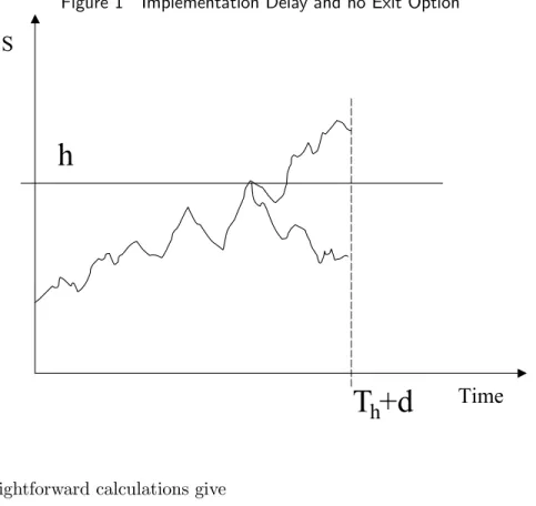
case gives us the value reduction associated with the implementation lag when there is no abandonment option. In this application, neither the operational division nor the headquarters have any profitability requirement once the investment decision as been taken optimally at Th(S). The delay with no exit option is illustrated in
Figure 1 on p. 24.
1 9
Figure 1 Implementation Delay and no Exit Option
h
Time
S
T
h
+d
Straightforward calculations give
A (θ) = e−ρd B (θ) = eγd
³
µ−σ22 (1−γ) ´
and the optimal investment boundary is
h∗(∆, Ce, d) = e−d ³ µ−σ2 2 (1−γ) ´ h∗(∆, Ce, 0)
This investment boundary is strictly lower than h∗(∆, Ce, 0) when γ > 0 if we
assume µ ≥ σ22. When there is an implementation delay, investors anticipate
in-vestment decisions by choosing an inin-vestment threshold lower than in the standard analysis. If we had µ ≤σ22, then we would expect to find a higher threshold.
Using equation 2.6, we see that the ratio of the value of the investment oppor-tunity with delay to that with no delay is
r (θ) = exp ½ dξ1 µ µ + σ 2 (γ − 1) 2 − ρ ξ1 ¶¾ .
Numerical simulations reveal that the implementation delay has an impact on the value of the investment opportunity. with reasonable parameters20 , we find that the ratio is about 94%. By changing the drift µ and increasing it to 5%, the ratio jumps to 98%. This illustrates how the delay can hurt the value of the investment if the state variable does not tend to increase significantly over the waiting period on average. The associated value reduction is due to the discount-ing of the investment NPV from Th to Th+ d and to the dependence of the value
of the project on the evolution of the decision variable during the implementation
2 0
period. The agent in charge with the investment decision does not benefit from the opportunity to abandon the project during the implementation lag. Further-more, since markets are incomplete, it is impossible for the firm to suppress the uncertainty concerning the evolution of the value of the decision variable during this period of time. Therefore, the value of the investment opportunity depends on the evolution of the decision variable21 over the time interval [Th, Th+ θ].
One can show that the value reduction due to the implementation delay is increasing as a function of the opportunity cost of capital for reasonable parameter values. As capital gets more costly, the effect of the discounting factor associated with the implementation period and the uncertainty concerning the profitability of the project weight more on the value of the investment opportunity.
European abandonment option
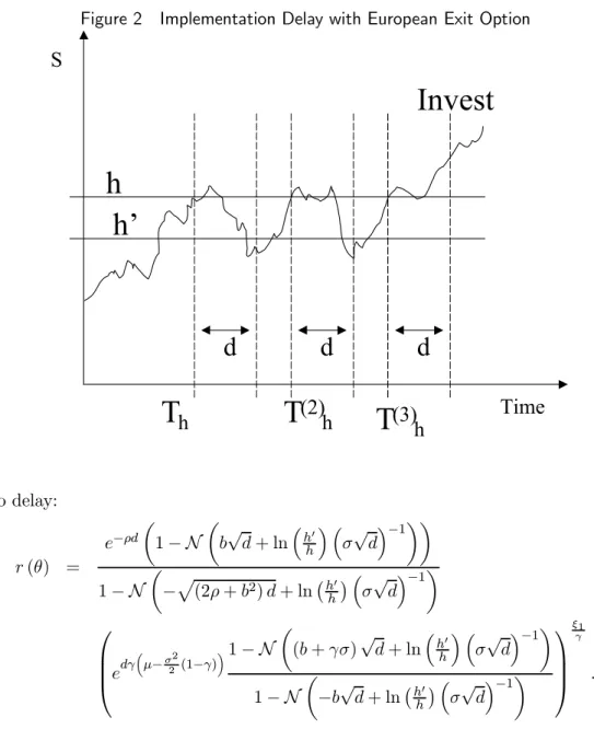
This application accounts for the case of an investment decision taken at division level that has to be approved by the headquarters. If the approval arrives d units of time after the submittance, then the operational manager invests only if the state variable is above a new cutoff level h0. The headquarters have no own profitability requirements during the implementation lag and the approval is based on the strategical merits of the project (new line of business, expanded markets). On the contrary, there are profitability requirements when the operational manager is in charge with the decision i.e. at times Th and Th+ d.
The variable θ, that is the time when the investment is decided, is here the first instant when d units of time after having hit h, the state variable is above h0, such that if it is not over h0, one has to wait until the process hits h again before re-waiting until it hits h again, and so on. Optimally, h0 is obviously expected to
be lower than h. Using the definitions from Chapter 3, we have θ = νhd0,h(S) . In Chapter 3, we show that S
νh0 ,hd is independent of ν h0,h
d (S) . The European
imple-mentation delay is shown in Figure 2 on p. 26.
Chapter 3 formally defines this stopping time and provides the tools to compute the law of this stopping time. Using Proposition 4 on p. 39, we get
A (θ) = e−ρd µ 1 − N µ b√d + ln³hh0´ ³σ√d´−1 ¶¶ 1 − N µ −p(2ρ + b2) d + ln¡h0 h ¢ ³ σ√d´−1 ¶ B (θ) = edγ ³ µ−σ22 (1−γ) ´1 − N µ (b + γσ)√d + ln ³ h0 h ´ ³ σ√d ´−1¶ 1 − N µ −b√d + ln¡hh0¢ ³σ√d´−1 ¶ .
where N is the Standard Normal cumulative distribution function N (x) = √1 2π Z x −∞ e−t22 dt, x ∈ R and b = µ− σ2 2
σ . We can find the ratio of the optimal value of the investment project
with European abandonment option to the value of the investment project with
2 1
The mean change in the decision variable during the implementation delay is given by eγd
µ µ−σ2
2(1−γ)
which is larger than one. Nevertheless, as the real path followed by the stochas-tic process ruling the evolution of this variable can be unfavorable to the firm, the abandonment options are not valueless.
Figure 2 Implementation Delay with European Exit Option
h
Time
S
T
h
d
h’
T
(2)
h
d
T
(3)
h
d
Invest
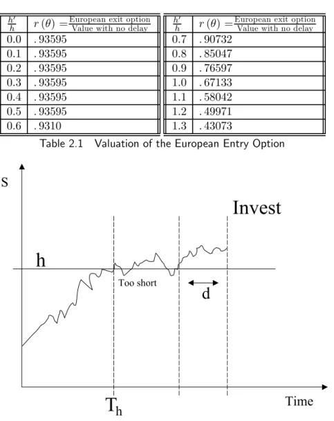
no delay: r (θ) = e−ρd µ 1 − N µ b√d + ln³hh0´ ³σ√d´−1 ¶¶ 1 − N µ −p(2ρ + b2) d + ln¡h0 h ¢ ³ σ√d´−1 ¶ edγ ³ µ−σ22 (1−γ) ´1 − N µ (b + γσ)√d + ln³hh0´ ³σ√d´−1 ¶ 1 − N µ −b√d + ln¡hh0¢ ³σ√d´−1 ¶ ξ1 γ .Numerical results show that this ratio is decreasing in h0/h. The European abandonment option will always be exercised as we have h0/h = 0 at the optimum. When the manager holds a European abandonment option, the value of waiting to invest at the maturity of this security (i.e. at the implementation date) is lower than the benefits of investing directly. Postponing the investment spending would lower the value of the profits generated by the investment project by an amount larger than an immediate exercise at Th+ d would. Table 2.1 on p. 27 shows
numerical results with the same parameters as in the preceding example.
As the European abandonment option is valueless, it is not optimal for the headquarters, once they have approved the project on its strategical merits, to have any profitability requirement at Th+ d if the investment decision has been
taken optimally at Th. In the same way, their is no interest for the firm to negotiate
with external investors the availability of this exit option at the end of the gathering of the funds when the investment project requires external financing.
The Parisian abandonment option
We give here the value of the investment opportunity when the manager invests at θ only if the decision variable reaches a prespecified level and remains above
h0
h r (θ) =
European exit option Value with no delay
0.0 . 93595 0.1 . 93595 0.2 . 93595 0.3 . 93595 0.4 . 93595 0.5 . 93595 0.6 . 9310 h0 h r (θ) =
European exit option Value with no delay
0.7 . 90732 0.8 . 85047 0.9 . 76597 1.0 . 67133 1.1 . 58042 1.2 . 49971 1.3 . 43073
Table 2.1 Valuation of the European Entry Option
h
Time
S
T
h
d
Invest
Too shortFigure 3 Implementation Delay with Parisian Option
this level for a time interval longer than a fixed amount of time (the window) without going back down. In this application, the time window is equal to the implementation delay and the prespecified level is set at an optimal value, the best investment threshold h∗. The decision triggering criterium is a so-called Parisian stopping time depending on the size of excursions of the state variable over the optimal investment threshold. We have θ = Hh,d+ (S), where Hh,d+ (S) is defined below. The Parisian abandonment option is represented graphically in Figure 3 on p. 27.
This investment criterion reflects the will of the investing firm (the headquarters and the operational division) to check that the market conditions remain favorable during the implementation lag. The firm has profitability requirements which are constant over time i.e. the level of the state variable has to stay above some constant cutoff level during the whole implementation lag. Intuitively, this cutoff level will be lower than the investment boundary of the standard case without implementation lag22.
2 2Note that this Parisian investment criterion is not absolutely optimal. It only uses one degree of freedom, that is the level of the barrier.
In order to find the value of the investment opportunity under the Parisian investment policy, we define the following random variables, all linked to a random process X:
gat(X) = sup {s ≤ t : Xs= a}
Ha,d+ (X) = inf {t ≥ 0 : (t − gta(X)) ≥ d, Xt≥ a} .
ga
t (X) represents the last time the process X crossed the level a. It can be checked
it is not a stopping time for the Brownian filtration Ft, but for the slow filtration
G = (σ (sgn (Bt)) ∨ Fgt)t≥0 which represents the information on the Brownian
motion until its last zero plus the knowledge of its sign after this23. Hh,d+ (X) is therefore the first instant when the process has spent d units of time consecutively over the level a.
Using the above notations, the Parisian investment policy is described by the stopping time Hh,d+ (S). In this case, the value of the investment opportunity can be written VP(S0, h, d, Ce) = ES0 h e−ρHh,d+ (S) ³ F³SH+ h,d(S), ∞ ´ − Ce ´i
The Parisian criterion allows for two degrees of freedom: the barrier h and the ”time window” d, which we naturally choose as the minimal implementation delay. Following the approach we outlined for the general model, we write for S0< h,
the value of the investment project as
VP (S0, h, ∆, Ce, d) = ES0 ·Z ∞ 0 dte−ρtf (St) It≥H+ h,d(S) ¸ − CeES0 h e−ρHh,d+ (S) i
Using the independence of the index paths after and before Hh,d+ (S), we can write the value of the investment opportunity as
VP(S0, h, ∆, Ce, d) = ES0 h e−ρHh,d+ (S) ³ F³SH+ h,d(S), ∞ ´ − Ce ´i Writing St= S0exp ¡ σZtb¢where Ztb = Bt+ bt and b = µ− σ2 2 σ , we have VP (S0, h, ∆, Ce, d) = ES0 · e−ρHa,d+ (Z b)µ F µ S0exp µ σZHb+ a,d(Zb) ¶ , ∞ ¶ − Ce ¶¸ with a = 1σln³Sh 0 ´
. Thanks to the equality in law between Ha,d+ ¡Zb¢and H0,d+ ¡Zb¢+ Ta³¡Zb¢0´, for two independent copies Zb and¡Zb¢0 , and thanks to the indepen-dence between ¡Zb t, t ≤ Ta ¢ and ¡Zb t, t ≥ Ta ¢ we get VP(S0, h, ∆, Ce, d) = ES0 · e−ρHa,d+ (Z b)µ F µ h exp µ σZHb+ 0,d(Zb) ¶ , ∞ ¶ − Ce ¶¸
Using the approach for the general model outlined in section 2 we have
VP(S0, h, ∆, Ce, d) = µ S0 h ¶ξ1 ES0 h e−ρH0,d+ (Z b)i ׳EhF³h exp³σ³bd + m1 √ d´´, ∞´i− Ce ´ . 2 3
d r (θ) Parisian r (θ) No exit 0.0 1.0 1.0 0.25 . 99931 . 98359 0.50 . 99333 . 96745 0.75 . 98464 . 95157 1.0 . 97415 . 93595 d r (θ) Parisian r (θ) No exit 1.5 . 94968 . 90548 2.0 . 92237 . 87601 3.0 . 86401 . 8199 10.0 . 50804 . 51587
Table 2.2 Valuation of the Parisian Entry Option
where m1 is the Brownian meander taken at time 1. The difficulty in the above
expression is to calculate the Laplace transform of the Parisian time H0,d+ ¡Zb¢. Thanks to the results of Chesney, Jeanblanc and Yor (1997) on Parisian options, we are able to directly write this value. The law of BH+
0,d was also derived in
Chesney, Jeanblanc and Yor (1997) and is given in Chapter 3. Using theorem 7 on p.43 (taken from Chesney, Jeanblanc and Yor (1997)) and after straightforward simplifications, we finally have
VP(S0, h, ∆, Ce, d) = µ S0 h ¶ξ1 Φ ³ b√d ´ Φ³pd (2r + b2)´ × ∆hγΦ ³ (σγ + b)√d´ Φ³b√d´ − Ce . where Φ (x) = Z +∞ 0 z exp µ zx − z 2 2 ¶ dz = 1 +√2πxe−x22 N (x) .
This can also be written as
A (θ) = Φ³b√d´ Φ³pd (2ρ + b2)´ B (θ) = Φ ³ (σγ + b)√d ´ Φ ³ b√d ´ .
The ratio of the value of the Parisian investment opportunity with respect to the investment opportunity with no delay, at their respective optima, is
r (θ) = Φ³b√d´ Φ³pd (2ρ + b2)´ Φ ³ (σγ + b)√d´ ³ Φ³b√d´´ ξ1 γ .
We can compare the value of the investment project with no delay, with a delay and no exit option (or a European option), and with a delay and a Parisian investmen criterion, see Table 2.2 on p. 29. We use the same parameters as in the preceding examples.
The value of the investment opportunity is shown to be higher when the in-vestor has the opportunity to choose the Parisian investment criterion than in the standard case, for reasonable parameter values. This investment policy gives the
investor the option to give up its investment opportunity if the decision variable goes below a prespecified level hP during the implementation of the investment spending. This option is freely obtained when the firm uses internal funds to fi-nance its investment opportunity. Therefore, the cost of outside funds is higher than traditionally assumed as they often prevent the management from exercising such embedded options. The value of the Parisian option gives us the maximum price that the firm will be willing to pay for this option to be available during the gathering of outside financing funds.
Numerical imulations indicate that when the delay becomes very long, it be-comes better to follow the European criterion, and invest as soon as the delay is expired. This leaves indeed a positive value for the project, while the Parisian criterion forces the investor to delay the investment too much: it becomes less and less likely that the state variable will spend consecutively a long period of time above the threshold.
When the investing firm holds a Parisian abandonment option, the optimal investment boundary is given by
hP (∆, Ce, d) = h∗(∆, Ce, 0) Φ ³ b√d´ Φ³(σγ + b)√d´ 1 γ
Since Φ (.) is a strictly increasing function, the investment boundary is lower than in the standard case with no implementation delay for γ > 0. One can notice that when d = 0, we find back the results associated with the standard case. Moreover, the larger the implementation lag, the lower the optimal investment barrier is and the lower the hurdle rate used by the firm. Note that if γ = 1, then the optimal barrier hP in the Parisian case is lower with respect to the non-delayed case by a factor that corresponds to how higher the state variable should be at the time of investment. On average, the investment decision will intervene at the same level as in the non-delayed case.
This investment criterion provides the value of the decision variable under which their will be no investment. According to this model there exists a value of waiting to invest but the real investment threshold and the option premium can vary according to the basic parameters and the shape of the excursion of the decision variable over the barrier. The value of the decision variable for which investment will occur and the value of the option premium can therefore be over or under the standard ones. This phenomenon has recently been stressed by the empirical evidence concerning real options (see Quigg (1993)).
American abandonment option with an exponential exercise barrier
When we look at standard results concerning American options, it is clear that the optimal exercise barrier exhibits some time dependence. Therefore, the Parisian criterion is not absolutely optimal as for the corresponding option the abandon-ment barrier is constant through time. Indeed, if for example the state variable goes back under the barrier just one day before the end of the implementation, it would not be optimal to cancel it. As a matter of fact, there exists a time depen-dence of the optimal abandonment level to how much time the firm has spent in the implementation of its investment decision.
In this section, we give the value of the investment opportunity if the man-ager invests at θ only if the decision variable remains above an early abandonment


![Table 5.1 on p. 83 represents the value of this factor, as a function of θ ∈ [0, 0.2]](https://thumb-eu.123doks.com/thumbv2/123doknet/14602252.731333/86.918.281.626.95.260/table-p-represents-value-factor-function-θ.webp)