HAL Id: hal-02493149
https://hal.archives-ouvertes.fr/hal-02493149
Submitted on 27 Feb 2020
HAL is a multi-disciplinary open access
archive for the deposit and dissemination of
sci-entific research documents, whether they are
pub-lished or not. The documents may come from
teaching and research institutions in France or
abroad, or from public or private research centers.
L’archive ouverte pluridisciplinaire HAL, est
destinée au dépôt et à la diffusion de documents
scientifiques de niveau recherche, publiés ou non,
émanant des établissements d’enseignement et de
recherche français ou étrangers, des laboratoires
publics ou privés.
Theoretical and Numerical Study of the Group Line
Florestan Platzer, Marc Saillard, Vincent Fabbro
To cite this version:
Florestan Platzer, Marc Saillard, Vincent Fabbro. Two-Dimensional Spectra of Radar Returns from
Sea: 1. Theoretical and Numerical Study of the Group Line. Journal of Geophysical Research.
Oceans, Wiley-Blackwell, 2019, �10.1029/2019JC015121�. �hal-02493149�
Two-Dimensional Spectra of Radar Returns from Sea: 1.
Theoretical and Numerical Study of the Group Line
F. Platzer1,2 , M. Saillard2 , and V. Fabbro1
1ONERA/DEMR, Université de Toulouse, Toulouse, France,2Université de Toulon, Aix Marseille Université, CNRS/INSU, IRD, MIO UM 110, Mediterranean Institute of Oceanography, La Garde, France
Abstract
The work presented here aims at interpreting the pattern observed at low frequencies in wavenumber-frequency (k, 𝜔) representations (dispersion diagrams) of radar returns from sea surface. This pattern is sometimes referred to as the “group line” in the literature and is supposed to result from the nonlinear behavior of the signal with respect to surface profile. To confirm this assumption, we have calculated the patterns generated by various nonlinear terms of second order in sea surface height. It is shown that the resolution in frequency of most data is not sufficient to allow for an accurate representation of the group line through an FFT. A methodology is proposed to define an average slope of the group line, which can be interpreted in terms of velocity.1. Introduction
Time series of microwave radar cross section (RCS) from sea surface are almost routinely used to image sea surface and extract informations about surface current or sea state, see for instance the review paper Borge et al. (2013) and references herein. Such radars operate in the microwave range and illuminate the surface under grazing incidence from a vessel or a platform. Data processing is often based on a Fourier transform in both range and time. The resolution in range of the radars are less than a few meters while time series dura-tion is about a few tens of seconds. The resulting 2D (or 3D) spectrum exhibits some characteristic patterns of gravity waves, including a bright line (or surface) in accordance with their dispersion relation, but also some energy along the harmonics and a so-called “group line” at low time and space frequencies. The group line results from the nonlinear dependence of the backscattered field with respect to surface parameters. If coherent radars are used, one can map either the radar cross section or the Doppler velocity, both lead-ing to similar plots Frazier and McIntosh (1996). Interpretation of the group line has been investigated in Frazier and McIntosh (1996), Smith et al. (1996), Plant and Farquharson (2012), with emphasis on the sig-nature of breaking waves or wave groups at the crest. It is also noticed that the group line occurs in slices of the 3D Fourier transform of optical measurements Leckler et al. (2015), but it seems that the authors have not focused their attention on it.
In Frazier and McIntosh (1996), the authors explore many explanations. After suggesting that “there is little doubt that the backscattered power profile has a nonlinear relation to local incidence angle” at grazing incidence, which is the preferred interpretation in the present paper, a detailed discussion about the velocity of non-Bragg contibutors that may be linked to breaking waves or scatterers bounded to the crest finally drives the reader to an interpretation in terms of hydrodynamic phenomena. The same year, Smith et al. Smith et al. (1996) also interpret the slope of the group line in terms of “group modulation of wave breaking,” since the associated velocity exceeds what would be expected from the modulation of Bragg wave.
More recently, Plant and Farquharson (2012) have excluded turbulent eddies in the wind, water turbulence advected by currents, second-order hydrodynamic or electromagnetic nonlinearities or shadowing as main contributors, while the latter has been considered as the dominant nonlinear mechanism in Borge et al. (2013). In Plant (2012), Plant establishes a correspondance between the slope of the group line, the velocity derived from Doppler spectra and the peak of Philips' Lambda function, introduced in Phillips (1985). In the wind direction, these quantities are close to each other, suggesting all of them bring the signature of breaking waves. However, numerical simulations of dispersion diagrams based on nonlinear Schrödinger equation do exhibit such features Krogstad and Trulsen (2010), for weakly nonlinear one-dimensional surfaces. This is also the case for the simulations presented here. Therefore, not only the interpretation of the group line
RESEARCH ARTICLE
10.1029/2019JC015121 This article is a companion to Platzer et al. (2019), https://doi.org/10.1029/ 2019JC015123.
Key Points:
• Two-dimensional spectra were extracted from radar returns from sea surface
• A pattern is observed at low frequencies in wavenumber-frequency spectra • The characteristics of this pattern
have been explicitly linked to the spectrum of waves
Correspondence to:
F. Platzer, M. Saillard and V. Fabbro, [email protected]; [email protected]; [email protected]
Citation:
Platzer F., Saillard, M., & Fabbro, V. (2019). Two-dimensional spectra of radar returns from sea: 1. Theoretical and numerical study of the group line. Journal of Geophysical Research:
Oceans, 124, https:// doi.org/10.1029/2019JC015121
Received 6 MAR 2019 Accepted 25 AUG 2019
Accepted article online 31 OCT 2019
©2019. American Geophysical Union. All Rights Reserved.
8767–8776.
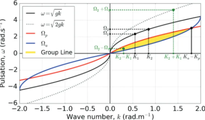
Figure 1. Geometrical description of the group line associated with a
band-limited continuous power spectrum.
still deserves to be discussed, but there is also some need for a clear def-inition of the slope of the group line, since it is associated to the velocity of waves.
In this paper, after the group line has been defined and exhibited in Section 2, we present in Section 3, for the one-dimensional case, a detailed theoretical analysis of the group line generated by a quadratic function of sea surface height or of its slope. The same calculations can be performed for any quadratic term involving the surface height and its time or spatial derivatives, but only these two have been of interest when compared to the data, in sections 6 and 7 at the end of the paper. This is also consistent with the discussions about the link between sea spikes, fast scatterers, and breaking waves which focus on large slopes and on the crests of high waves. In Section 4, it is shown that the fast Fourier transform (FFT) of experimental time series lacks of resolution in frequency to provide an accurate description of the group line. However, an empirical formula is given in Section 5, which avoids tedious computations for a huge set of frequencies.
2. Group Line
This section focuses on the group line generated by a nonlinear function of a random variable with Gaussian probability density and given power spectrum S(K), typically a linear superposition of gravity waves or the associated distributions of slopes. Since the radar resolution in range is about 1 m, or more, smaller scales are filtered out from S and capillary waves are not considered. On the low frequency side, the spec-trum is assumed to vanish very rapidly below the wavenumber Kpassociated with the dominant wave.
The calculations performed here thus apply to typical spectra of wind waves and do not take into account the superposition of swell.
At large depths and without current, the dispersion relation of gravity waves is Ω =√gK, K =|K| and Ω denoting the wavenumber and the frequency, respectively.
In the frame of linear approximation, the contribution to surface height of waves longer than the radar resolution in range, characterized by the high-wavenumber cutoff Ku, can be written as
𝜂L(x, t) = ∫ K<Ku
A(K) exp(iK. x − iΩ(K)t)dK + cc, (1) where|A| is the square root of the spectrum of surface gravity waves and Ω(K) is given by the dispersion relation of gravity waves.
To understand the influence of nonlinearities and the characteristics of the group line, let us first con-sider the simple case of a quadratic dependence 𝜂2
L. For simplicity, let us combine two periodic waves
Figure 2. Example of dispersion diagram derived from experimental data
Fabbro et al. (2017).
propagating in the same direction, 𝜂1(K1, Ω1) and 𝜂2(K2, Ω2).
The product 𝜂1𝜂2 generates terms with wavenumbers K = ±K2±K1and associated frequencies Ω = ±Ω2±Ω1= ±√gK2±√gK1. If K1 and K2 are close to each other, the resulting points in the (k, 𝜔)
plane are close either to the second harmonic𝜔 = ±√2gkor to the origin. The slope of the straight line joining the origin to the latter is nothing but the group velocity of the wave packet.
Let us now keep k = K2−K1constant and increase K1from Kpup to Ku,
where Kpis the low frequency cutoff of the spectrum of gravity waves.
Since shorter waves than Ku are discarded here, A(K1)A*(K
2)vanishes
when K1lies out of the interval [Kp, Ku−k].|Ω2− Ω1| is thus decreas-ing from𝜔p =
√
g(Kp+k) −√gKpdown to𝜔u =√gKu−√g(Ku−k). Consequently, for a wide-band spectrum, the group line fills a part of the (k, 𝜔) plane of which pattern is controlled by the long energetic waves on one side (Kp), the resolution in range on the other side (Ku), as illustrated
Journal of Geophysical Research: Oceans
10.1029/2019JC015121
Figure 3. Dispersion diagram of the computed backscattered amplitude for
1D sea surface with wind speed 7 m/s, illuminated under grazing incidence and H polarization at L band. The resolution in range is 1.25 m. Horizontal axis: wavenumber; vertical axis: frequency.
since only A(K) is modified in this case. Diagrams from real data, such as the one in Figure 2 computed through a 2D FFT of range-time series from the database described in Fabbro et al. (2017), do exhibit a cloud of energetic points at low space and time frequencies. The boundaries of the group line do not clearly appear, because of noise, of poor resolution, and of the direction spreading of gravity waves.
Similar plots are also obtained from a numerical solver based on a rigorous boundary integral formalism, devoted to scattering from one-dimensional rough surfaces illuminated under grazing incidence Miret et al. (2014). In Figure 3, sea surface is described by Pierson Moskowitz spectrum and computations are performed for horizontal polarization at L band. Creamer's approach is used to represent hydrody-namic nonlinearities Creamer et al. (1989). The contribution from each range cell is recorded during about 1 min, and a two-dimensional FFT is then performed. It is interesting to notice that the group line is clearly vis-ible, even though hydrodynamic nonlinearities are assumed to be weak and no breaking occurs. This result is consistent with the theoretical predictions of Krogstad and Trulsen (2010).
In the two-dimensional case, the Fourier transform with respect to x of𝜂2
Lis nothing but the autoconvolution
of A(K) exp(−iΩ(K)t) (defined equation (1)),
̃𝜂2
L(k, t) = ∫ ∫ K<Ku
A(K)A(k− K) exp(−i(Ω(K) + Ω(k − K))t)dK + cc
+ ∫ ∫K<KuA(K)A∗(K− k) exp(−i(Ω(K) − Ω(K − k))t)dK + cc, (2) where K refers to wavenumber of waves while k refers to the Fourier coordinate. A second Fourier transform with respect to t leads to Dirac distributions𝛿 (𝜔 ± (Ω(K) + Ω(k − K))) and 𝛿 (𝜔 ± (Ω(K) − Ω(k − K))). Only the second one provides values of𝜔 located below the dispersion relation 𝜔 =√gkand contributes to the
Figure 4.|A(K)A(K − k)|versus Kx∕Kpand Ky∕Kp, fork = Kp̂xwith peak
wave Kp=0.1and phase speed to wind speed ratio cp∕U=0.75. A is assumed to follow the empirical spectrum proposed by Hasselmann Hasselmann et al. (1980);82%of the integral is concentrated between the white lines with slopes±tan𝜋∕6. The distribution becomes even narrower when k is increased.
group line. If, instead of𝜂2
L, a quadratic function involving slopes is
considered, the spectrum of gravity waves has to be replaced by the corresponding moment.
In the following, we will focus our attention on the case where the radar beam propagates in the direstion of the wind. In these conditions, k lies along this direction and the quantity A(K)A*(K − k) that contributes to
the group line takes significant values when K is also directed in this direction and decays rapidly away from it, as shown in Figure 4 for typ-ical weather conditions encountered during data measurements Fabbro et al. (2017). In addition, since𝜔 = Ω(K) − Ω(K − k) is an even function of K⟂, the component of K perpendicular to k, we have𝜕K𝜕𝜔
⟂(K⟂=0) = 0.
It results that𝜔 is almost unchanged when K slightly deviates from wind direction. Therefore, it seems reasonable in this case to perform the analytical estimation of the group line in the frame of a 1D problem.
3. Analytical Results
Here, it is assumed that all the wavevectors are aligned along the x axis, oriented according to wind direction. Since ̃̃𝜂2
L(k, 𝜔) = ̃̃𝜂L2 ∗
(−k, −𝜔), we can restrict our investigations to k ≥ 0. In this case, the 2D FFT̃̃𝜂2
Lcan
be calculated exactly. Indeed, only one value of K between Kp+kand Ku satisfies𝜔 − Ω(K) + Ω(K − k) = 0, as required by the Dirac distribution.
Figure 5. Group line associated with𝜂2
L(log scale) for a band-limited K−3
wave spectrum. The low-frequency cutoff is Kp=0.14rad∕m and the radar range resolution, acting as high-frequency cutoff, is Ku=1rad∕m. The blue line represents the weighted average value,< 𝜔 > (k).
From,𝜔 =√gK −√g(K − k), it comes once squared, √ g(K − k) = √ gk 2 ( √ gk 𝜔 −√𝜔gk ) (3) √ gK = √ gk 2 ( √ gk 𝜔 +√𝜔gk ) . (4)
Therefore, if S(K) is a power-law spectrum which behaves as K−𝛼and with
A(K) ∝√K−𝛼, |A(K)A∗(K − k)| ∝ k−𝛼(gk 𝜔2− 𝜔 2 gk )−𝛼 . (5)
In addition, since𝜔(K) is a single valued invertible function, the contri-bution of̃̃𝜂2
L(k, 𝜔) to the group line is
||
||dKd𝜔||||A(K)A
∗(k − K) (6)
with|A(K)A*(k − K)| given by equation (5). The derivative of equation (4) with respect to 𝜔 gives
|| ||dKd𝜔||||= k 2𝜔 (gk 𝜔2− 𝜔 2 gk ) (7) resulting in || ||A(K)A∗(K − k)dK d𝜔||||∝ k1−𝛼 𝜔 ( gk 𝜔2− 𝜔 2 gk )1−𝛼 . (8)
An example is given in Figure 5, which exhibits the group line derived from equation (6), for a band-limited K−3spectrum. The plot has been restricted to the upper right quadrant, since the spectrum
is centro-symmetric and all the waves go in the same direction here. To translate this 2D map in terms of “velocity,” the weighted average< 𝜔 > is calculated for each k,
< 𝜔 >= ∫ 𝜔p 𝜔u 𝜔||||̃̃𝜂 2 L(k, 𝜔)||||d𝜔 ∫𝜔p 𝜔u || ||̃̃𝜂L2(k, 𝜔)||||d𝜔 , (9)
and the mean slope< 𝜔 > ∕k between 0 and k is considered. In Figure 5, < 𝜔 > has been plotted, according to the following formula, derived after tedious calculations
< 𝜔>𝜂2 L= √ gk [ 𝜔 √ gk 1−(𝜔2gk)2 −1 4ln 1+√𝜔 gk 1−√𝜔 gk −1 2arctan 𝜔 √ gk ]𝜔u 𝜔p [ 1 1− ( 𝜔2 gk )2 ]𝜔u 𝜔p , (10) where𝜔p= √ g(Kp+k) − √ gKpand𝜔u= √ gKu− √
g(Ku−k)are the upper and lower boundaries of the
domain covered by the group line, respectively.
The same kind of calculations can be performed for the square of the slope,𝜂2
Lx(𝜂x= 𝜕𝜂𝜕x). In this case, since
the spectrum has a slower decay, as K−1, equation (8) takes a very simple form, namely, 1∕𝜔. As a result the energy density of the group line spreads out in a more homogeneous way, leading to smaller values of< 𝜔 > than for𝜂2
Journal of Geophysical Research: Oceans
10.1029/2019JC015121
Figure 6. Average slope of the group line< 𝜔 > ∕kversus k for a band-limited K−3spectrum with K
p=0.14rad∕m.
Blue line: slope of̃̃𝜂2
Lfor Ku=1; cyan line: the same for Ku=2𝜋; red line: slope of𝜂̃̃2Lxfor Ku=1; green line: the same
for Ku=2𝜋. < 𝜔>𝜂2 Lx= [𝜔]𝜔u 𝜔p [ln𝜔]𝜔u 𝜔p . (11)
The difference between the group lines associated with𝜂2
Land𝜂Lx2 is illustrated in Figure 6, which compares
both average slopes< 𝜔 > ∕k. The high sensitivity of the group line of 𝜂2
Lxto the high-frequency cutoff is
also exhibited in Figure 6, where both cases Ku=1and Ku=2𝜋 have been considered. The higher Ku, the
smaller slope. This results from the slow decay of the spectrum of𝜂Lx, of which rms depends on Ku.
On the contrary, the slope of the group line of𝜂2
Lis hardly changed, because most of the energy is
concen-trated along the line𝜔 = 𝜔p(k). It is also worth to notice that the limit when k tends to 0 of< 𝜔 > in equation (10) is 0.4√g∕Kpk, leading to slope at origin 0.4c𝜙(Kp)for𝜂2Lin Figure 6, where c𝜙(Kp) =
√ g∕Kp
denotes the phase velocity of the most energetic wave. This is a little less than its group velocity cg=c𝜙∕2, because of the weight of slower waves of sea spectrum. The 0.4 coefficient is thus the signature of the K−3
decay of the spectrum. Let us also point out that the slope decreases with k.
Similar analytical calculations can be done for other types of second-order terms, such as𝜂2
Ltor𝜂L𝜂Lx, but
such calculations become too complicated for higher order nonlinearities. However, it has been observed that the dispersion diagrams derived from experimental data present very small amount of energy in the vicinity of higher harmonics (Figure 2), suggesting that second-order terms are the leading nonlinearities.
4. Synthetic Data
Range-time series of 𝜂L(x, t) have also been generated numerically through the superposition of time-harmonic waves with random phases. It appears that for usual durations of recording, typically a minute, the dispersion plots derived from 2D FFT significantly differs from the previous analytical results. The discrepancy is reduced when very long time series are considered.
To understand the origin of this behavior, let us come back to Figure 1 in Section 2, where we have pointed out that, for given k,𝜔 = √g(k + K) −√gK is slowly decreasing toward zero when K increases. More precisely, since the derivative of equation 4 gives
dK d𝜔 = − k 2𝜔 ( gk 𝜔2− 𝜔 2 gk ) , (12)
the interval dK which feeds the range of frequencies [𝜔 − d𝜔, 𝜔] behaves as 𝜔−3for small values of𝜔.
There-fore, when performing a time FFT, with resolution𝛥𝜔 = 2𝜋∕T where T denotes the duration of the time series, the contributions from large wavenumbers, for instance K1=Kuand K2=Ku−k, can be separated
if T > √8𝜋 gk (K u k )3∕2
Figure 7. Comparison of theoretical and computed average slopes of the
group line< 𝜔 > ∕kversus k, for𝜂2
Lx(blue: Ku=1; red: Ku=2𝜋).
experiments have shown that an accurate computation of the integral is even more demanding. So a few minutes long time series do not allow an accurate representation of the group line generated by high-resolution radars. Obviously, the 2D FFT underestimates the contribution from low frequencies. This explains why the numerical estimation of< 𝜔 > is greater than the exact value and why the discrepancy is greater for Ku=
2𝜋 than for Ku = 1in Figure 7, where 400 s long time series have been
considered. In the same way, the error is much lower when considering𝜂2 L
than𝜂2
Lx, since the weight of low frequencies is smaller in the former case.
Hence, we can conclude that the 2D FFT is not suited to study the group line generated from real data. As a consequence, quantitative estimation of physical parameters such as velocity of waves or breakers from such a representation is not relevant.
5. Empirical Formula to Correct 2D FFT Output
For such “short” time series, numerical experiments have shown that the group line derived from the 2D FFT presents a behavior that can be fitted with analytical formula. For instance, when considering the group line associated with𝜂2Lx, the average
frequency< 𝜔 > (k) follows with very good accuracy
< 𝜔 >= 3 [ 𝜔5∕2]𝜔p 𝜔u 5[𝜔3∕2]𝜔p 𝜔u (13)
instead of equation (11). Though we have no mathematical proof, everything occurs as if dk∕d𝜔 behaves as𝜔−3/2instead of𝜔−3(equation 12). This rule also works for𝜂2
L, leading to replace equation (10) by the
formula given in Appendix A
As an example, Figure 8 exhibits the agreement between the empirical formula and computations of the 2D FFT of short synthetic range-time series. Displacements of 500 m long surface profiles have been recorded during 400 s. Averaging is performed over 200 of such surfaces. To sum up the results presented in the last two sections, Figure 9 presents how the predictions of the 2D FFT evolves from the empirical formula at low recording durations down to the theoretical result of Fourier analysis at very long ones. Accuracy at very low values of k is hard to achieve, since a small fluctuation of< 𝜔 > generates a large deviation of < 𝜔 > ∕k. Hence, we have now at hand a way to transform the average value of𝜔 derived from FFT of range-time series with poor resolution in frequency into the one that should result from Fourier transform of an infinitely
Figure 8. Comparison of empirical formula and computed average slopes
of the group line< 𝜔 > ∕kversus k, for𝜂2
Lx. The solid lines represent the
computed average slopes while the circle markers represent the empirical formulas.
long time series, through multiplication by the ratio equation (11) /equation (13). This step is essential if one aims at giving physical inter-pretation of the data.
6. Comparison with Data from Numerical Solution
of the Scattering Problem
To check the validity of the previous results, we have tested them against the group line derived from numerical solution of the scattering problem, as already exhibited in Figure 3. The computation provides time series of the backscattered amplitude from each radar cell. A dispersion diagram is obtained through a 2D FFT and the average value< 𝜔 > (k) is computed from equation (9), where the square height has been replaced by the radar cross section. In Figure 10, the group line associated with the backscat-tered field from 100 radar cells, each 1.25 m in length, recorded during 1 min, is presented. The radar frequency is 1.2 GHz and its polarization is horizontal. In Miret et al. (2014) Tatarskii and Charnotskii (1998), it has been demonstrated that the backscattered amplitude from a rough
Journal of Geophysical Research: Oceans
10.1029/2019JC015121
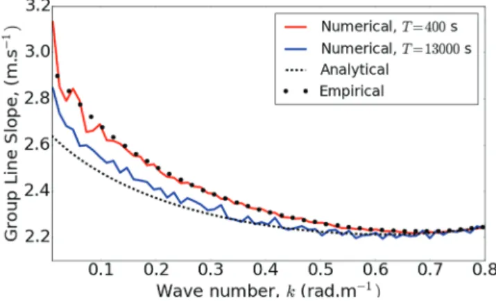
Figure 9. Comparison of theoretical, empirical, and computed average
slopes of the group line< 𝜔 > ∕kversus k, for𝜂2Lx(Ku=1). (blue: Tint=13, 000s; red: Tint=400s).
surface separating two homogeneous media behaves as the square of the vertical component of the incident wavevector when the grazing inci-dence angle tends toward zero. In the present model, the hydrodynamic nonlinearities are assumed to be weak and the surface profile remains smooth. The assumption of a boundary separating two homogeneous media is thus fulfilled. If one extends the limiting behavior of the scatter-ing amplitude for each radar cell of sea surface, even if it is much smaller than the wavelength of long gravity waves, it comes that the fluctuations of the scattering amplitude with range follow that of the square of the ver-tical component of the local incidence wavevector. Keeping in mind that the slope of gravity waves remain low, the local incidence angle remains low as well. Therefore, denoting by𝜃0the grazing incident angle, the
backscattered amplitude from a radar cell is proportional to the square of the local grazing angle
s0(x) ∝ (sin𝜃
0+𝜂Lx(x))2 (14)
of which first nonlinear term with respect to sea surface profile is𝜂2 Lx.
Therefore, since the time series is short, the average frequency derived from the scattering computations (blue solid line) has to be com-pared with the one predicted by the empirical formula established for the square of surface slope𝜂2
Lx
(equation (13)). A very good agreement is observed.
7. Comparison of the Slope of the Group Line with the Velocity of Breakers
Coherent radars permit one to get also range-time maps of the velocity, defined as the first moment of the Doppler spectrum. Their frequency-wavenumber spectra have been studied in Plant (2012), where it is noticed that the slope of the group line compares with the most probable velocity of breaking gravity waves c0. In Irisov and Plant (2016), the authors have fitted the set of c0data with a second-order polynomial in c𝜙(Kp), the phase velocity of the dominant wave,c0=0.22 + 0.39c𝜙−0.008c2𝜙. (15)
It is interesting to notice that the first order coefficient is very close to the slope at k = 0 of< 𝜔 > in equation (10), which is equal to 0.4. This suggests to compare c0 with the slope associated with𝜂2
L.
Since the second-order derivative of < 𝜔 > at k = 0 is negative, we have found a small value of k which allows us to fit the polynomial, as shown in Figure 11. Although choosing k = 0.11 is not based on physical considerations, noticing that the group line in Figure 2 or in figure 1 of Plant (2012) con-centrates energy between k = −0.2 and k = 0.2, it makes sense to estimate the slope in this range. But the most important here is that we get the same behavior and the same order of magnitude over a very wide range of values of c𝜙(Kp). Therefore, if the radar echo is dominated by the contribution
of breakers and if c0 is a good approximation of their velocity, it may be conjectured that the group
Figure 10. Focus on the group line computed from the solution of the scattering problem. White solid line: average
Figure 11. Slope of the group line< 𝜔 > ∕k(equation (10)) versus phase velocity of the dominant wave c𝜙(Kp)(red), for k around 0.11, versus the empirical formula proposed in Irisov and Plant (2016) for the most probable velocity of breakers (solid line).
line of the dispersion diagram of the average Doppler velocity should behave as the one derived from 𝜂2
L.
8. Conclusion
The characteristics of the group line have been explicitly linked to the spectrum of waves, at least for simple nonlinear functions of𝜂. Since the group line is not a single line but an area of the (k, 𝜔) plane, a systematic procedure has been proposed to give a mathematical sense to the “slope of the group line,” to allow its inter-pretation in terms of velocity. Applying numerical 2D fast Fourier transform to data with coarse frequency grid leads to overestimate the slope and to misinterpret the associated velocity. A correction must be applied to make the numerical result consistent with that derived from a Fourier transform.
Since the amplitude of the backscattered electromagnetic field is a nonlinear function of surface profile, the 2D dispersion diagram derived from the Fourier transform in range and time always exhibit a group line, whatever the sea surface state. In the particular case of low grazing incidence, when the asymptotic regime predicted in Tatarskii and Charnotskii (1998) is reached, numerical simulations provide consistent results, the slope of the group line fitting the one generated by the square of the slope of long gravity waves𝜂2
Lx.
Finally, it has been noticed that the behavior of the slope of the group line associated with𝜂2
L, with respect
to phase velocity of the dominant wave, fits well the most probable velocity of breakers, as estimated in Irisov and Plant (2016). Since the computations performed here are restricted to weak hydrodynamic non-linearities, we have not been able to exhibit group lines with such high slopes. This will be investigated in a companion paper focusing on in situ data analysis Platzer, Fabbro, & Saillard, 2019. (submitted).
Appendix A
Equations (9, 11, 13) require analytical calculation of integrals of the type I(𝛽, n) = ∫ 𝜔𝛽 ( gk 𝜔2− 𝜔 2 gk )−n d𝜔, (A1)
with𝛽 = −1, 0,12,32and n = 0or2.
Below is given the average value of𝜔 for the group line associated with 𝜂2
Lwhen a 2D FFT is used to compute
the dispersion diagram.
Journal of Geophysical Research: Oceans
10.1029/2019JC015121
with N = I(32, 2) and D = I(12, 2). N =√gk ⎡ ⎢ ⎢ ⎢ ⎣ 8 ( 𝜔 √ gk )5∕2 1 −(√𝜔 gk )4+5 ln 1 −√𝜔 gk 1 +√𝜔 gk ⎤ ⎥ ⎥ ⎥ ⎦ 𝜔p 𝜔u +√gk ⎡ ⎢ ⎢ ⎢ ⎣ 10 √ 2 arctan ⎛ ⎜ ⎜ ⎜ ⎝ √ 2𝜔 √ gk 1 −√𝜔 gk ⎞ ⎟ ⎟ ⎟ ⎠ −10 arctan √ 𝜔 √ gk ⎤ ⎥ ⎥ ⎥ ⎦ 𝜔p 𝜔u +√gk ⎡ ⎢ ⎢ ⎢ ⎣ 5 √ 2 ln 1 +√2√𝜔 gk+ 𝜔 √ gk 1 −√2√𝜔 gk+ 𝜔 √ gk ⎤ ⎥ ⎥ ⎥ ⎦ 𝜔p 𝜔u (A3) D = ⎡ ⎢ ⎢ ⎢ ⎣ 8 ( 𝜔 √ gk )3∕2 1 −(√𝜔 gk )4+3 ln 1 −√𝜔 gk 1 +√𝜔 gk ⎤ ⎥ ⎥ ⎥ ⎦ 𝜔p 𝜔u + ⎡ ⎢ ⎢ ⎢ ⎣ 6 arctan √ 𝜔 √ gk −√6 2 arctan ⎛ ⎜ ⎜ ⎜ ⎝ √ 2𝜔 √ gk 1 −√𝜔 gk ⎞ ⎟ ⎟ ⎟ ⎠ ⎤ ⎥ ⎥ ⎥ ⎦ 𝜔p 𝜔u + ⎡ ⎢ ⎢ ⎢ ⎣ 3 √ 2 ln 1 +√2√𝜔 gk+ 𝜔 √ gk 1 −√2√𝜔 gk+ 𝜔 √ gk ⎤ ⎥ ⎥ ⎥ ⎦ 𝜔p 𝜔u (A4) with𝜔p= √ g(Kp+k) − √ gKpand𝜔u= √ gKu− √ g(Ku−k).References
Borge, J. N., Reichert, K., & Hessner, K. (2013). Detection of spatio-temporal wave grouping properties by using temporal sequences of x-band radar images of the sea surface. Ocean Modelling, 61, 21–37. https://doi.org/10.1016/j.ocemod.2012.10.004
Creamer, D. B., Henyey, F., Schult, R., & Wright, J. (1989). Improved linear representation of ocean surface waves. Journal of Fluid
Mechanics, 205, 135–161. https://doi.org/10.1017/S0022112089001977
Fabbro, V., Biegel, G., Förster, J., Poisson, J. B., Danklmayer, A., Böhler, C., et al. (2017). Measurements of sea clutter at low grazing angle in mediterranean coastal environment. IEEE Transactions on Geoscience and Remote Sensing, 55(11), 6379–6389. https://doi.org/10.1109/ TGRS.2017.2727057
Frazier, S. J., & McIntosh, R. E. (1996). Observed wavenumber-frequency properties of microwave backscatter from the ocean surface at near-grazing angles. Journal of Geophysical Research, 101(C8), 18,391–18,407. https://doi.org/10.1029/96JC01685
Hasselmann, D. E., Dunckel, M., & Ewing, J. A. (1980). Directional wave spectra observed during jonswap 1973. Journal of Physical
Oceanography, 10(8), 1264–1280. https://doi.org/10.1175/1520-0485(1980)010<1264:DWSODJ>2.0.CO;2
Irisov, V., & Plant, W. (2016). Phillips' lambda function: Data summary and physical model. Geophysical Research Letters, 43, 2053–2058. https://doi.org/10.1002/2015GL067352
Krogstad, H. E., & Trulsen, K. (2010). Interpretations and observations of ocean wave spectra. Ocean Dynamics, 60(4), 973–991. https:// doi.org/10.1007/s10236-010-0293-3
Leckler, F., Ardhuin, F., Peureux, C., Benetazzo, A., Bergamasco, F., & Dulov, V. (2015). Analysis and interpretation of frequency-wavenumber spectra of young wind waves. Journal of Physical Oceanography, 45, 2484–2496. https://doi.org/10.1175/ JPO-D-14-0237.1
Miret, D., Soriano, G., & Saillard, M. (2014). Rigorous simulations of microwave scattering from finite conductivity two-dimensional sea surfaces at low grazing angles. IEEE Transactions on Geoscience and Remote Sensing, 52(6), 3150–3158. https://doi.org/10.1109/TGRS. 2013.2271384
Phillips, O. M. (1985). Spectral and statistical properties of the equilibrium range in wind-generated gravity waves. Journal of Fluid
Mechanics, 156, 505–531. https://doi.org/10.1017/S0022112085002221
Plant, W. J. (2012). Whitecaps in deep water. Geophysical Research Letters, 39, L16601. https://doi.org/10.1029/2012GL052732, l16601 Plant, W. J., & Farquharson, G. (2012). Origins of features in wave number-frequency spectra of space-time images of the ocean. Journal of
Geophysical Research, 117(C6), C06015. https://doi.org/10.1029/2012JC007986
Acknowledgments
The authors acknowledge the Délégation Générale de l'Armement (DGA) for financial support and Gabriel Soriano, at Institut Fresnel, for valuable discussions and for providing the computer code devoted to solving the scattering problem. The data used in the paper are not available publicly. These are the property of Fraunhofer FHR, WTD71, and ONERA. Please contact the authors at [email protected] for more information.
Platzer, F., Fabbro, V., & Saillard, M. (2019). Two-dimensional spectra of radar returns from sea: Analysis of the group line from experimental data. Journal of Geophysical Research: Oceans, 124. https://doi.org/10.1029/2019JC015123
Smith, M., Poulter, E., & McGregor, J. (1996). Doppler radar measurements of wave groups and breaking waves. Journal of Geophysical
Research, Oceans, 101(C6), 14,269–14,282. https://doi.org/10.1029/96JC00766
Tatarskii, V. I., & Charnotskii, M. I. (1998). On the universal behavior of scattering from a rough surface for small grazing angles. IEEE