Centroid-aware local discriminative metric learning in speaker verification.

HAL Id: hal-01769892

https://hal-univ-tln.archives-ouvertes.fr/hal-01769892

Submitted on 17 May 2018

HAL is a multi-disciplinary open access

archive for the deposit and dissemination of

sci-entific research documents, whether they are

pub-lished or not. The documents may come from

teaching and research institutions in France or

L’archive ouverte pluridisciplinaire HAL, est

destinée au dépôt et à la diffusion de documents

scientifiques de niveau recherche, publiés ou non,

émanant des établissements d’enseignement et de

recherche français ou étrangers, des laboratoires

Centroid-aware local discriminative metric learning in

speaker verification.

Kekai Sheng, Weiming Dong, Wei Li, Joseph Razik, Feiyue Huang, Baogang

Hu

To cite this version:

Kekai Sheng, Weiming Dong, Wei Li, Joseph Razik, Feiyue Huang, et al.. Centroid-aware local

discriminative metric learning in speaker verification.. Pattern Recognition, Elsevier, 2017, 72 (c),

pp.176-185. �10.1016/j.patcog.2017.07.007�. �hal-01769892�

Centroid-Aware Local Discriminative Metric Learning

in Speaker Verification

Kekai Shenga,b, Weiming Donga,∗, Wei Lic, Joseph Razikd, Feiyue Huangc, Baogang Hua,b

a_{LIAMA-NLPR, Institute of Automation, Chinese Academy of Sciences, Beijing, China} b_{University of Chinese Academy of Sciences}

c_{Laboratory Youtu, Tencent Inc., Shanghai, China} d_{Laboratory LSIS, University of Toulon, Toulon, France}

Abstract

We propose a new mechanism to pave the way for efficient learning against class-imbalance and improve representation of identity vector (i-vector) in au-tomatic speaker verification (ASV). The insight is to effectively exploit the in-herent structure within ASV corpus — centroid priori. In particular: 1) to ensure learning efficiency against class-imbalance, the centroid-aware balanced boosting sampling is proposed to collect balanced mini-batch; 2) to strengthen local discriminative modeling on the mini-batches, neighborhood component analysis (NCA) and magnet loss (MNL) are adopted in ASV-specific modi-fications. The integration creates adaptive NCA (AdaNCA) and linear MNL (LMNL). Numerical results show that LMNL is a competitive candidate for low-dimensional projection on i-vector (EER=3.84% on SRE2008, EER=1.81% on SRE2010), enjoying competitive edge over linear discriminant analysis (LDA). AdaNCA (EER=4.03% on SRE2008, EER=2.05% on SRE2010) also performs well. Furthermore, to facilitate the future study on boosting sampling, connec-tions between boosting sampling, hinge loss and data augmentation have been established, which help understand the behavior of boosting sampling further. Keywords: Text-Independent ASV, Centroid-Aware Balanced Boosting Sampling, Adaptive Neighborhood Component Analysis, Linear MagNet

1. INTRODUCTION

Automatic speaker verification (ASV) is an important yet difficult pattern recognition task, and it can be divided into two categories: text-dependent ASV and text-independent one. We focus on the latter task in this work. An ASV system is usually composed of two modules: one is front-end for acoustic

∗_{Corresponding author}

feature extraction and voice activity detection (VAD), and the other is back-end for representation extraction (e.g., i-vector [1]) and similarity measure.

Figure 1: Feature visualization (t-SNE) [2] of i-vectors from the background corpus in National Institute of Standards and Technology speaker recognition evaluation (SRE) 2010 (left ) and the corresponding histogram of numbers of instances of each speaker (right ).

Technically, ASV systems are susceptible to intersession variability (intra-speaker variability [3, 4] and inter-(intra-speaker one [5]), causing local confusions (left of Fig. 1). Class-imbalance is another issue (right of Fig. 1), being counter-productive to learning as the training signal can be biased by class-imbalance data. To improve results against the issues, many methods [6, 7, 8, 9, 10] have been proposed. Amongst the previous literature of improved representation of i-vector space, it is observed that the adverse effect of class-imbalance seems to have received little attention. But we argue that class-imbalance does inhibit optimization progress and render the representation space of not discrimination enough, especially when the amount of data is limited (e.g., SRE 2008).

With the point in mind, we try to investigate how to improve the i-vector space and eschew class-imbalance simultaneously. The key idea here is to pro-pose a mechanism efficiently exploiting the centroid-priori of ASV corpus [11]. In particular: 1) centroid-aware balanced boosting sampling collects class-balance mini-batches for efficient learning process, and 2) neighborhood component anal-ysis (NCA) [12] or magnet loss (MNL) [13] strengthens local discriminative mod-eling on the mini-batches. Integrating the two modules creates adaptive NCA (AdaNCA) and linear MNL (LMNL). Comparisons with several typical metric learning methods demonstrate the effectiveness of our mechanism.

The main contributions of this work are summarized as follows:

1 Centroid-aware balanced boosting sampling is developed to mollify class-imbalance and pave the way for efficient learning, like hard example mining. 2 AdaNCA and LMNL based on NCA and MNL are developed with

ASV-specific modifications to strengthen local discriminative modeling.

3 Connections are established between boosting sampling, hinge loss and data augmentation to further reveal the behavior of boosting sampling.

The rest of the paper is organized as follows. Section 2 introduces the related works. Section 3 describes the problem setting and the proposed mechanism.

Figure 2: Illustration of the pipelines of the training stage of the mechanism (instance sampling + local discriminative modeling) and the validation stage in ASV task scenarios.

Section 4 presents details of the experiments and Section 5 summarizes useful knowledge in ASV. Section 6 carries out further investigation on the boosting sampling strategy. Section 7 elaborates the conclusions and future works.

2. RELATED WORKS 2.1. I-vector in ASV

Identity vector (i-vector) [1], also known as total variability modeling, aims to model the utterance variability in a low-dimensional space. Total variability originates from joint factor analysis, and the model is represented as

M(s) = m + T · ω(s), (1) where s denotes a target speaker; m is a speaker-/channel-independent super-vector, which is taken from a universal background model (UBM) supervector; T is the total factor matrix, which is an expanded subspace of speaker-/channel-dependent information; ω(s) is the i-vector extracted from the input utterance (details are available in [14]). I-vector has proved to be an effective represen-tation for the inherent information of speakers (see e.g., [15, 16, 17]).

As previously noted, however, the performance degradation in ASV systems is attributed to the two issues. Many researchers attempt to mollify the issues with metric learning techniques, such as linear discriminant analysis (LDA), nearest neighbor discriminant analysis (NDA) [18] for low-dimensional projec-tion on i-vector, or probabilistic LDA (PLDA) [7, 19] for intersession variability compensation. In this work, we resort to better representation of i-vector space and tackle class-imbalance issue at the same time to encourage the optimization to progress further, resulting in improved ASV result.

2.2. Distance metric learning

Distance metric learning aims at learning a transformation to a representa-tion space where the distance corresponds with a task-specific norepresenta-tion of simi-larity. Classical examples of this research field are listed as follows.

Given the set of N (i-vector, label) pairs {(xi, yi)}N

i=1, LDA is commonly used for low-dimensional projection on i-vector before PLDA in ASV for the sake of computational efficiency. NDA [20] models the variances based on K nearest neighbors (KNN) of xi, N NK(xi), to better preserve the local data structure. NCA [12] is another scheme used to train the linear transformation A on nearest neighbors modeling (i.e., pij in Eq. 2), which is akin to t-SNE [2] — i.e., a useful technique to unveil the structure in data.

f (A) = N X i=1 pi = N X i=1 X j∈{l|yl=yi} pij, with pij= exp(−kAxi− Axjk22) P k6=iexp(−kAxi− Axkk22) (pii= 0) (2)

Weighted class-oriented linear regression [21] and fast NCA (FNCA) [22] leverage adaptive weighted learning to reinforce the local awareness of models. Large margin nearest neighbor (LMNN) [23] learns the transformation with two parts in Eq. 3 (µ denotes the tradeoff):

L(A) = (1 − µ) · Lpull(A) + µ · Lpush(A) (3)

where Lpull(A) pulls instances of identical class closer and Lpush(A) pushes data of different label farther. Comparatively, stochastic triple embedding [24] learns the representation in a triplet manner, and joint Bayesian model (JBM) starts from a different assumption to obtain success in face verification task [25]. Magnet loss (MNL) [13] and lifted structured feature embedding [26] are two latest well-designed methods for enhanced local discrimination modeling.

In ASV scenarios, NDA has proved to be a strong substitute for LDA [18]. It should be noted that, the exploitation of the local data structure is at the heart of the success of NDA. Inspired by NDA and the recently successful applications of local discriminative modeling (see e.g., [13, 27, 28]), we desire to improve the representation of i-vector space by virtue of the local discriminative modeling in exploiting the inherent structure in ASV data.

2.3. Sampling strategies in stochastic gradient descent

Mini-batch stochastic gradient descent (SGD) is an optimization algorithm and has proved to be beneficial to various tasks [29]. Eq. 4 shows the idea:

Wk+1= Wk− λk· ( 1 |Bk| X xi∈Bk ∇L(xi, Wk)) (4)

where Bk denotes the mini-batch, Wk is the weight being optimized at step k with learning rate λk; L(xi, W ) refers to the loss given data xi and weights W . Since random shuffling is unable to ensure training efficiency against un-desirable properties in data (e.g., noise or redundancy) in many tasks, many researchers strengthen the training signal via better mini-batches. For example, Shrivastava et al. [30] made it through an online hard example mining method.

Yang et al. [31] enhanced the optimization efficiency by proposing drop-sample algorithm. Miguel et al. [27] leveraged complete-linkage cluster to discover com-pact data cliques and enabled CNNs in exemplar learning. Can´evet et al. [32] regarded the problem in collecting false positives as an exploitation (focus on false positives) versus exploration (use the entire data) dilemma and applied Monte Carlo tree search to solve it. They share one idea: well-selected unbi-ased mini-batch Bk possesses obvious advantage over randomly-selected ones in ensuring the quality and learning efficiency of models. With this view, the approach to collect Bk is generally task-specific and worthy of effort.

Inspired by the idea, to prevent the gradient estimates from being vitiated by the imbalance corpus and exploit the benefit in online mini-batch selection for learning efficiency, we need to develop an effective class-balance sampling strategy during the course of optimization in ASV setting.

3. PROBLEM SETTING AND MODIFICATIONS 3.1. Problem setting

Considering N (i-vector, label) pairs {(xi, yi)}N_i=1, where xi∈ Rdivector _and

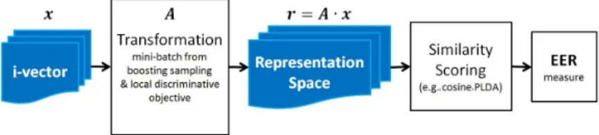
yi∈ {1, · · · , Nclass}, we train a linear transformation A with an objective or loss (e.g., LMNL Eq. 8 and AdaNCA Eq. 7) for a transformed space {ri= A·xi}Ni=1, where ri∈ Rdprojection, with a low equal error rate (EER, the error value when the false acceptance rate is equal to the false rejection rate after adjusting the threshold value). Fig. 3 shows the pipeline.

Figure 3: Workflow of experiments with distance metric learning in ASV.

In the test/validation stage, the similarity between two instances is:

di,j(A) = rTi · rj=

xT

i · ATA · xj

kAxik2· kAxjk2

. (5)

Cosine metric, Eq. 5, is adopted for similarity scoring to reveal the discrimina-tion of the representadiscrimina-tion. To further ensure the necessity of the low-dimensional projection from A in the ASV community — i.e., whether lower EER can be achieved — PLDA should be performed on the transformed space.

As mentioned previously, the main purpose of this work is to better ASV results with improving representation of i-vector while boosting optimization ef-ficiency against class-imbalance. We propose a mechanism to attain the goal by exploiting the inherent structure in ASV data. Specifically, centroid-aware sam-pling (see Sec. 3.2) generates genuinely hard unbiased mini-batch to ensure the

learning efficiency, and local discriminative objective (see Sec. 3.3) is introduced to help strengthen local discriminative modeling on the mini-batches.

The motivations behind the combination are twofold. First, a well-designed sampling strategy is a promising solution to ensure the training efficiency of models, especially when there is class-imbalance issue or when there are much more easy examples than meaningfully hard ones, which would weaken the train-ing signal. Second, a local discriminative objective can effectively absorb the information from mini-batches of the collected genuinely hard instances (e.g., high error) and result in a better representation space, leading the sampling process to mine for other confusable neighbor structures. Therefore, we believe that the integration of the solutions helps get the best of both worlds.

3.2. Centroid-aware balanced boosting sampling

In this section, we describe the centroid-aware balanced boosting sampling algorithm, which uncovers the internal structure within ASV corpus to combat class-imbalance for efficient learning. The pseudocode is shown in Alg. 1.

The motivation behind Alg. 1 is: clustering is a natural avenue to reveal the inherent data structure, as it can organize data into cliques and make it easy to detect the confusing regions, akin to hard example mining [30, 31]. However, it may also incur undesirable high computational workload. To avoid extra clustering computation cost, we propose three techniques as follows:

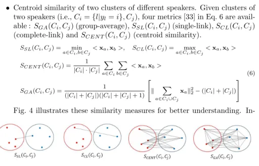
• Centroid similarity of two clusters of different speakers. Given clusters of two speakers (i.e., Ci= {l|yl= i}, Cj), four metrics [33] in Eq. 6 are avail-able : SGA(Ci, Cj) (group-average), SSL(Ci, Cj) (single-link), SCL(Ci, Cj) (complete-link) and SCEN T(Ci, Cj) (centroid similarity).

SSL(Ci, Cj) = min a∈Ci,b∈Cj < xa, xb>, SCL(Ci, Cj) = max a∈Ci,b∈Cj < xa, xb> SCEN T(Ci, Cj) = 1 |Ci| · |Cj| X a∈Ci X b∈Cj < xa, xb> SGA(Ci, Cj) = 1 (|Ci| + |Cj|)(|Ci| + |Cj| + 1)  k X a∈Ci∪Cj xak22− (|Ci| + |Cj|)   (6)

Fig. 4 illustrates these similarity measures for better understanding.

In-Figure 4: Schematic illustrations of the four similarity measures: single-link similarity, complete-link similarity, centroid similarity, and group-average similarity.

tuitively, different measures uncover different aspects of data, and it’s the specific task that determines which is the best (e.g., SSL(Ci, Cj) for ag-glomerative clustering; SCL(Ci, Cj) for compact cliques detection [27]).

Algorithm 1 Centroid-aware balanced boosting sampling

Require: {xi, yi}Ni=1; A; C = {Cj = {i | yi = j}}Nj=1class (Nclass refers to the total number of different classes in the corpus); F = {Fj ∈ {0, 1}}Nclass

j=1 records whether the class j has been sampled during sampling for a single mini-batch, and index(1:M ·D) records data indexes in a single mini-batch; In each mini-batch: M is the number of different classes and D denotes the number of samples of identical label; Nbatch refers to the number of mini-batches (for computational efficiency and stable training dynamics) Ensure: vector of indexes of samples in mini-batches indexmini−batch_{(1:M ·D)}

1: Perform length-normalization {ˆri← A·xi

kA·xik2}

N

i=1 for feature comparability

2: Initialize the array of sampling flags Fi← 0 (i = 1, · · · , Nclass)

3: Initialize indexmini−batch_{(1:M ·D)} and index(1:M ·D)as empty vector

4: Generate L ← {(i, j, SCEN T(Ci, Cj)) | i, j ∈ {1, 2, · · · , Nclass} and i < j}

5: Sort L in a descend manner by SCEN T(Ci, Cj)

6: while L is not empty and |indexmini−batch_{(1:M ·D)} | < Nbatch do

7: pop one tuple (i, j, SCEN T(Ci, Cj)) from the top of L

8: if Fi== 0 and |Ci| ≤ D and |index(1:M ·D)| < M · D then

9: randomly pick D indexes out of Ci and stack them into index1:M ·D

10: Fi← 1 // 1 for being sampled yet

11: end if

12: do the same on class Cj as lines 8 to 11

13: if |index(1:M ·D)| == M · D then

14: Stack index(1:M ·D) into indexmini−batch(1:M ·D)

15: re-initialize Fi (line 2) and reset index(1:M ·D) as an empty vector

16: end if

17: end while

18: return indexmini−batch_{(1:M ·D)}

In this case, we choose SCEN T(Ci, Cj). As centroid prior is intrinsic in ASV data [11] and SCEN T(Ci, Cj) can be aware of the centroid of speakers (evidence in Section. 5). That is why Alg. 1 is called centroid-aware. • Class-balance boosting sampling with replacement. Essentially,

class-imbalance decreases the ratio of hard examples as training progresses, and then models succumb to the biased training signal. So we’d better focus on the instances of large error to learn the fastest and eventually the best [34]. To this end, we generate mini-batches in a pairwise, hard-instance-first and class-balance manner. In particular, we evaluate SCEN T(Ci, Cj) of pairs of different speakers (line 4 of Alg. 1), sort them in descending order (line 5 of Alg. 1), and maintain class-balance of each mini-batch (lines 6 to 17 of Alg. 1). Replacement strategy (according to {Fj}Nclass

j=1 in Alg. 1) is also adopted to equip models with the capability to reuse critical data points adaptively, and consequently, we can boost the training efficiency further. • Random sampling as a regularizer. There is always some overfitting or oscillatory training dynamics coming with boosting sampling. To combat the detrimental effect, we perform random sampling (lines 9 to 10 of Alg. 1) in mini-batch generation. We believe that random sampling can help generate relatively unbiased mini-batches and make the gradient directions more explorative (e.g., less overfitting) to mitigate overfitting, working better than nearest neighbor sampling (e.g., NDA [18] or FNCA [22]). Combine the aforementioned techniques and we propose Alg. 1, the sampling strategy in our optimization process. The algorithm is able to incorporate useful data structures, i.e., class-balance meaningfully hard mini-batches, into a local adaptive metric for deeper optimization while keeping the computational cost tolerable. We share the same idea with Allen-Zhu et al. [35] that the optimal sampling process corresponds to gathering more instances of larger gradient contribution. Furthermore, the encoded sampling encourages models to learn in an ensemble manner for high model stability and low generalization error.

Class-aware sampling [36] is most closely related to Alg. 1. However, our method is endowed with SCEN T(Ci, Cj), boosting sampling and replacement strategy, which are useful techniques in encouraging the optimization to progress. No shuffle operation is performed on all the mini-batches, as our empirical results show that keeping the order of mini-batches boosts the training effectiveness. 3.3. Objective selection and modifications

As for the other module of our mechanism, we introduce two objectives — NCA [12] and MNL [13] — to strengthen local discriminative modeling. The reasons for the choices are twofold. First, a desirable representation modeling should originate from the inherent structure in data. Being independent of any task-free data assumption means that the model can get rid of the limitations from the predefined assumptions and mine the internal data structure directly. Consequently, the representation space from the model can be consistent with

the real data distribution. Second, for the sake of local discrimination, a desired objective should be aware of the internal structure in data, neither simply pair-wise [23] nor triplet-pair-wise [37]. Intuitively, such awareness can lead to a promising remedy for local discriminative modeling on i-vector space.

In this case, centroid priori is associated with ASV corpus [11] and readily available. Hence, NCA and MNL are two promising objectives to formalize the idea: NCA [12] performs the modeling on neighbor assignment akin to t-SNE, and MNL [13] offers a promising approach to take advantage of centroid prior. Given one mini-batch Si in indexmini−batch(1:M ·D) from Alg. 1, their ASV-specific modifications, AdaNCA in Eq. 7 and LMNL in Eq. 8, are shown as follows.

ˆ A = arg max A 1 Z X j∈Si X k∈{a|ya=yj,a6=j}∩Si exp(−_2σ12kA · (xj− xk)k22) P l∈Si,l6=jexp(− 1 2σ2kA · (xj− xl)k22) with Z = M · D, µ(xi) = 1 D X j∈{l|yl=yi} xj, σ = 1 Z − 1 X j∈Si kA · (xj− µ(xj))k22

s.t. : Si= indexmini−batch_{(1:M ·D)} [i] f rom Alg.1

(7)

where µ(xi) refers to the centroid of class of xi, σ is a normalization factor to facilitate local discriminative modeling for a given mini-batch Si.

ˆ A = arg min A 1 Z M X m=1 D X d=1 {− log exp(− 1 2σ2krmd − µmk 2 2− α) P µ:C(µ)6=C(rm d)exp(− 1 2σ2krmd − µk 2 2) }+ with Z = M · D, rm_d = A · xm_d, µm= 1 D D X d=1 rm_d, σ = 1 Z − 1 M X m=1 D X d=1 krm_d − µmk22

s.t. : xmd denotes the representation of dthindex of mthclass in Si,

Si= indexmini−batch_{(1:M ·D)} [i] f rom Alg.1

(8)

where C(·) denotes the class ID of input (given a centroid µ, C(µ) refers to the class ID from which we calculate µ); α is the margin in hinge loss.

To our knowledge, this paper is the first to leverage MNL in ASV setting. We choose to adopt MNL without deep learning and provide mini-batches via Alg. 1 to work better in ASV scenarios. The results help better understand MNL and provide valuable knowledge for enhancing ASV systems.

4. EXPERIMENT CONFIGURATIONS 4.1. Corpora usage

Generally, the corpus for ASV task contains three disjoint sets: development set, enrollment set and trial set. The development set is utilized for training UBM, i-vector extractor and others techniques (e.g., LDA, PLDA) in the back-end; the remaining two sets are used to estimate the generalized performance of a given ASV system.

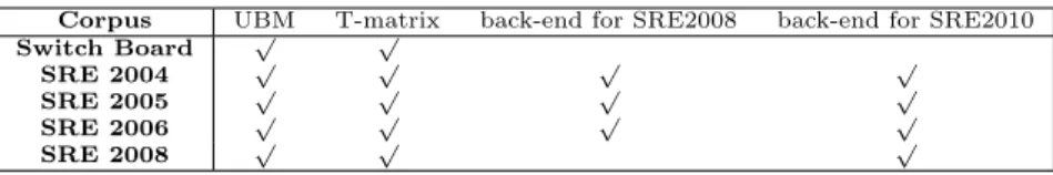
Information about the corpus usage is summarized in Table 1. All available corpora are collected to achieve good results, whereas a few useless (e.g., near silence or laughter) or poor (e.g., strong echo or noise) utterances are omitted to eliminate their negative effects on the training process.

Corpus UBM T-matrix back-end for SRE2008 back-end for SRE2010 Switch Board √ √ SRE 2004 √ √ √ √ SRE 2005 √ √ √ √ SRE 2006 √ √ √ √ SRE 2008 √ √ √

Table 1: Corpora for different modules during experiments on SRE2008 and SRE2010.

4.2. Experimental setup: front-end and i-vector extraction

In the experiments, MFCCs of 20 dimensions (19 + energy) on the win-dow of 20 ms with 10 ms shift are augmented with their delta and double delta coefficients, producing 60-dimensional feature vectors. Then, the feature vectors are subjected to feature warping. Prior to short-time cepstral mean and variance normalization, silence in recordings is trimmed with VAD. Subse-quently, gender-independent UBM (full covariance 2048 component GMM) and gender-dependent i-vector (di−vector=600) extractors are trained. On the basis of i-vector (EER=6.41% on SRE2008 and EER=6.23% on SRE2010), several different metric learning methods are performed for improved representation space and better ASV results. The code for feature extraction, VAD, and i-vector processes (e.g., training and extraction) comes from kaldi [38], a popular toolkit for speech recognition and speaker verification. Hence our baseline ASV system is guaranteed to be realistic.

Male telephone data (det6) from core condition (short2-short3) on SRE2008 and male telephone data (det5) on SRE2010 are used in the evaluation, and EER is evaluated based on the scores from Eq. 5.

4.3. Configurations of methods in the experiments

Given the non-convexity in AdaNCA and LMNL, SGD with momentum is utilized for optimization purpose. For a good initialization of A to encour-age convergence of training, we leverencour-age the orthogonal matrix from LDA to initialize A, similar to Dehak et al.[16], since LDA has demonstrated obvious improvements on i-vector and training stability. Besides, the normalization pre-process (zero-average normalization and length normalization) on i-vectors should be performed prior to the training to facilitate optimization progress.

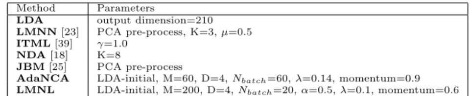
In addition to the proposed mechanism, various metric learning methods 1 are taken into account (see Table 2 for the specific parameter setting) in compar-ison experiments to figure out the key in optimizing the transformation in ASV. Moreover, we believe that a wide range of methods, different assumptions (e.g., LDA, NDA [18], ITML [39] and JBM [25]) or representation modeling (e.g., LMNN [23], AdaNCA and LMNL), can collaborate precisely as exploratory techniques to understand the inherent structure in data and provide enlighten-ing insights for further development in ASV systems.

1_{We adopt the code sources online: LDA in kaldi, Matlab toolbox for dimensionality}

Method Parameters

LDA output dimension=210 LMNN [23] PCA pre-process, K=3, µ=0.5 ITML [39] γ=1.0

NDA [18] K=8

JBM [25] PCA pre-process

AdaNCA LDA-initial, M=60, D=4, Nbatch=60, λ=0.14, momentum=0.9

LMNL LDA-initial, M=200, D=4, Nbatch=20, α=0.5, λ=0.1, momentum=0.6

Table 2: Parameter setting of various distance metric learning methods in experiments.

5. RESULT ANALYSIS

Important information of various metric learning methods (i.e., their proper-ties and ASV results) is organized in Table 3 for comparison. To further verify the role of AdaNCA and LMNL in ASV community, we perform PLDA on the raw i-vectors (to check the necessity of low-dimensional projection) and the representations after low-dimensional projection (LDA, AdaNCA and LMNL).

Locality Parametric Sampling SRE2008 SRE2010 Modeling distribution method cosine ( PLDA ) cosine ( PLDA ) i-vector 6.41% (5.61%) 6.23% (1.98%) LDA √ 4.69% (4.00%) 2.55% (1.99%) LMNN [23] √ random 8.88% 10.40% ITML [39] √ 15.98% 12.75% NDA [18] √ √ nearest 5.49% 2.55% JBM [25] √ 6.89% 3.08% AdaNCA √ Alg. 1 4.38% (4.03%) 2.34% (2.05%) LMNL √ Alg. 1 4.24% (3.84%) 2.29% (1.81%)

Table 3: Comparison of different metric learning methods on i-vector representation and their corresponding verification performance (EER) on SRE2008 and SRE2010. The dimension of the PLDA speaker subspace remains the same as the dimension of input representation.

The table shows considerable valuable knowledge on ASV as follows: • Local structure modeling is critical in improving representation of i-vector.

NDA (variances from nearest neighbors), AdaNCA (neighbor assignments with pij), and LMNL (centroid priori within ˆµm) adopt different local discrimination modeling, and they generally outperform global discrimi-nation methods in EER. Specifically, LMNL builds a better representation of i-vector to enable PLDA to achieve lower EER performance. Therefore, the proposed mechanism (boosting sampling + local discriminative mod-eling) is very competitive and efficient in ASV task scenarios.

Besides the good results, it’s also observed that when M or D increases too high or diminishes too small in Alg. 1, or when Bk are randomly collected, the learning efficiency is poor and the learned models always result in high EER. That is, the improper exploitation of the hard mini-batches (e.g., too greedy or too weak) results in poor explorative properties in SGD progress (e.g., underfitting), and subsequently, models tend to converge on local minima of high EER. Hence, it is clear that a proper approach for exploitation of the inherent structures in ASV corpus requires some efforts and we provide an applicable mechanism that is worthy of reference.

• Priority should be given to intra-class variation. In AdaNCA or LMNL, models prefer to pull instances of the same label closer than to push in-stances of impostor farther, as the gradient signal from neighbors of the target speaker generally surpasses that from non-target ones. Their suc-cesses imply that the pull force from target speakers makes more contri-butions to useful gradient estimates than the push force from non-target speakers does. Intuitively, the push force from a great number of non-target instances is prone to be contaminated by noise.

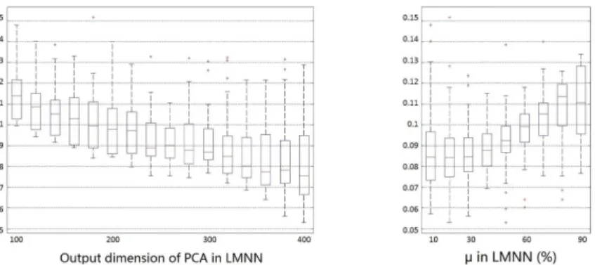
To analyze the contribution of pull or push force quantitively, we resort to LMNN — Lpull(A) and Lpush(A) easy the analysis. We train LMNN in various hyper-parameters (K∈{1, 3, 5}, µ∈{0.1, · · · , 0.9} and PCA di-mension ∈{100, 110, · · · , 400}), and the results are shown in Fig. 5. Two

Figure 5: Box plots of EER of LMNN with different settings of parameters on SRE2008. EER goes with the output dimension of PCA (Left ) and EER goes with the µ (Right ).

box plots show the influence of each hyper-parameter on the ASV perfor-mance. The tradeoff value, µ, in Eq. 3 of around 0.3 appears to be the best, suggesting that Lpull(A) from the same speaker takes more credits than Lpush(A) from samples of different impostors for promising results. • SCEN T(Ci, Cj) reveals more useful internal structures for ASV than others in Eq. 6. As noted before, measures in Eq. 6 lead models to focusing on dif-ferent aspects of data. Experimental results show that SCEN T(Ci, Cj) ex-hibits training stability and low EER. Comparatively, SGA(Ci, Cj) presents higher EER (about 0.2% higher than SCEN T) and reaches the training convergence at a slower rate; SSL(Ci, Cj) and SCL(Ci, Cj) seem to be vulnerable to data noise and even render the optimization oscillatory, re-sulting in EER values just moderately lower than the baseline.

Fig. 6 also buttress the role of centroid in ASV setting: mean-shift per-forms satisfactory in modeling the data distribution of i-vectors. In spite of some misfits, a large ratio of speakers properly center around each corre-sponding centroid. So it is arguable that exploiting centroid prior within the mini-batch generation or the objective function helps obtain accurate representation modeling and promote ASV performance.

Figure 6: T-SNE visualization on i-vectors from the background set of SRE2010 (green points) and the results (blue points) of mean-shift. Although a few mismatches are found, large parts of the centroid successfully cover a single local region of i-vectors of the same speaker.

6. FURTHER INVESTIGATION ON BOOSTING SAMPLING Since the integration of two solutions has proved to be effective for ASV task, a natural question follows: can we find some equivalence between sam-pling process (e.g., Alg. 1) and local discriminative objective (e.g., Eq. 3)? In what follows, we provide insights into the behavior of boosting sampling by es-tablishing its connections with hinge loss and data augmentation. The insights can shed a new light on boosting sampling strategy.

6.1. Hinge loss and boosting sampling

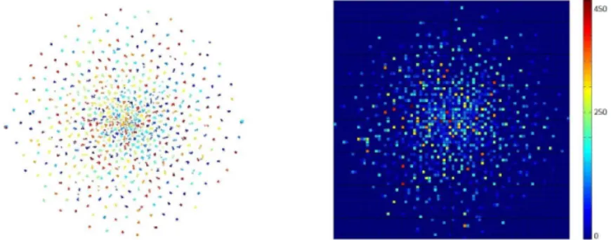
As the visualization in Fig. 7 shows: with the help of sampling algorithm, models tend to pour more attention on regions of similar impostors while ignor-ing easy-to-classify areas. That is, both AdaNCA and LMNL are only triggered

Figure 7: A schematic illustration of centroid-aware balanced boosting sampling working in a similar way to hinge loss. T-SNE visualization on i-vectors from SRE2008 (left ) and the corresponding heatmap of frequency data being sampled as SGD iterations proceed (right ).

Alg. 1, and LMNL filters indexmini−batch_{(1:M ·D)} further with hinge loss. Thus, some connections exist between boosting sampling strategy and hinge loss.

Another evidence comes from the derivative functions: hinge loss (Eq. 9; α is the margin) and loss function based on the collected set from sampling (Eq. 10) both emphasize on instances with large gradients to perform better near the decision boundary.

L(y) =X

i

max(0, α − ti· yi), (ti= ±1, yif or a classif ier score)

∂` ∂w= X i −ti·1{α > tl· yl} · ∂yi ∂w = X i∈{l|tl·yl<α} −ti· ∂yi ∂w (9) Lsampling(y) = X i∈collected set

L(yi), (yif or a classif ier score)

∂Lsampling ∂w = X i∈collected set ∂L ∂yi ·∂yi ∂w (10)

They are almost the same when the collected set — collected via a certain mini-batch generation algorithm — is {l|tl· yl < α}. Furthermore, they are also reciprocal: boosting sampling collects meaningful mini-batches from corpus for hinge loss, and hinge loss filters the mini-batches further (as LMNL does in Eq. 8). Many researchers integrate hard example mining into their models as an indispensable step for promising results. For instance, Chen et al. [40] proposed double-header hinge loss with hard quadruplets based on sampling for significantly large margin and computational efficiency.

On this basis, a connection is established between boosting sampling and hinge loss, and it can lead to better design of the optimization process. 6.2. Data augmentation and boosting sampling with replacement

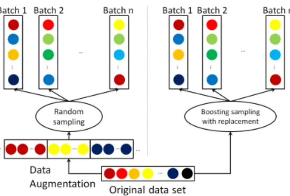
There is also a link existing between boosting sampling and data augmen-tation. This deduction is best illustrated with the two case studies in Fig. 8. In the left branch, each utterance generates several artificial copies to appear in different mini-batches without changing the labels. In the right branch, boost-ing samplboost-ing with replacement enables the model to adaptively reuse critical instances. They both allow every instance to contribute to the training signal several times in each SGD iteration over the whole development set. Moreover, boosting sampling with replacement helps mollify the challenges in designing augmentation (e.g., how and how many). Thus, boosting sampling with re-placement encodes data augmentation into optimization without the need for a specific augmentation strategy.

In fact, we tried to augment the extracted i-vectors from ASV corpus us-ing a class invariant method 2_{, but models suffer from those artificial copies}

2_{We randomly sample approximately 70% of the original frames from each utterance for}

50 copies and extract the corresponding i-vector. Given that the artificial i-vectors are closely similar to the original one, the augmentation strategy will not change the correct class.

Figure 8: Data augmentation (left ) and boosting sampling with replacement (right ) allow a single training sample to contribute to the learning in different mini-batches.

and EER decreases. Therefore, boosting sampling with replacement strategy is a preferable choice in ASV and other SGD methods, especially no effective augmentation strategy is available.

7. CONCLUSION AND FUTURE WORKS

In this paper, an effective mechanism is proposed to ensure learning efficiency against class-imbalance and improve local discriminative modeling on the repre-sentation space of i-vector, resulting in competitive EER results. Specifically, we develop the centroid-aware balanced boosting sampling to gather class-balance hard mini-batches to pave the way for efficient optimization. Next, we choose NCA and MNL for representation modeling to absorb the meaningful infor-mation in the mini-batches. The combination results in AdaNCA and LMNL. AdaNCA (EER=4.03% on SRE2008, EER=2.05% on SRE2010) and LMNL (EER=3.84% on SRE2008, EER=1.81% on SRE2010) both enjoy strong com-petitive performances and keep the computational workload low at the same time. Several typical metric learning methods are also compared to ensure the conclusion, and comparison experiments offer useful knowledge for further devel-opment in ASV task. Besides, we investigate the behavior of boosting sampling strategy further by establishing its connections with hinge loss and data aug-mentation. The connections can help us design improved optimization process with boosting sampling.

The results in this work can be improved with deep learning techniques fur-ther, and call for additional efforts in designing better approaches to exploit the intrinsic data structure — e.g., more effective hard example mining or objectives using centroid priori — in ASV task.

ACKNOWLEDGEMENT

This research is supported in part by National Natural Science Foundation of China (NSFC) (Grant No.: 61573348, 61620106003, 61672520), and in part

by the Institute of Automation Chinese Academy of Sciences (CASIA)-Tencent Youtu Joint Research Project. The authors are grateful to Fan Tang at CASIA, Fuzhang Wu, Xingming Jin, Peng Li, and others at Youtu Lab, Tencent Inc. for meaningful discussions and help. Besides, the authors thank all reviewers for their valuable comments on improving the quality of this paper.

References

[1] M. Senoussaoui, P. Kenny, N. Dehak, P. Dumouchel, An i-vector extrac-tor suitable for speaker recognition with both microphone and telephone speech, in: Odyssey, 2010, p. 6.

[2] L. v. d. Maaten, G. Hinton, Visualizing data using t-SNE, Journal of Ma-chine Learning Research 9 (Nov) (2008) 2579–2605.

[3] J. H. Hansen, Analysis and compensation of speech under stress and noise for environmental robustness in speech recognition, Speech communication 20 (1) (1996) 151–173.

[4] F. Kelly, A. Drygajlo, N. Harte, Speaker verification in score-ageing-quality classification space, Computer Speech & Language 27 (5) (2013) 1068–1084. [5] N. Dehak, Z. N. Karam, D. A. Reynolds, R. Dehak, W. M. Campbell, J. R. Glass, A channel-blind system for speaker verification, in: IEEE Interna-tional Conference on Acoustics, Speech and Signal Processing (ICASSP), 2011, pp. 4536–4539.

[6] G. Liu, Y. Lei, J. H. L. Hansen, Robust feature front-end for speaker iden-tification, in: 2012 IEEE International Conference on Acoustics, Speech and Signal Processing (ICASSP), 2012, pp. 4233–4236.

[7] S. J. D. Prince, J. H. Elder, Probabilistic linear discriminant analysis for inferences about identity, in: IEEE 11th International Conference on Com-puter Vision, 2007, pp. 1–8.

[8] P. Kenny, Bayesian speaker verification with heavy-tailed priors, in: Odyssey, 2010, p. 14.

[9] A. O. Hatch, S. S. Kajarekar, A. Stolcke, Within-class covariance normalization for svmbased speaker recognition, in: INTERSPEECH 2006 -ICSLP, 2006.

[10] F. Richardson, D. Reynolds, N. Dehak, Deep neural network approaches to speaker and language recognition, IEEE Signal Processing Letters 22 (10) (2015) 1671–1675.

[11] M. Senoussaoui, P. Kenny, T. Stafylakis, P. Dumouchel, A study of the cosine distance-based mean shift for telephone speech diarization, IEEE/ACM Transactions on Audio, Speech, and Language Processing 22 (1) (2014) 217–227.

[12] J. Goldberger, G. E. Hinton, S. T. Roweis, R. Salakhutdinov, Neighbour-hood components analysis, in: Advances in Neural Information Processing Systems, 2004, pp. 513–520.

[13] O. Rippel, M. Paluri, P. Dollar, L. Bourdev, Metric learning with adaptive density discrimination, in: International Conference on Learning Represen-tations (ICLR), 2015.

URL http://adsabs.harvard.edu/abs/2015arXiv151105939R

[14] P. Kenny, G. Boulianne, P. Dumouchel, Eigenvoice modeling with sparse training data, IEEE Transactions on Speech and Audio Processing 13 (3) (2005) 345–354.

[15] G. Liu, J. H. Hansen, An investigation into back-end advancements for speaker recognition in multi-session and noisy enrollment scenarios, IEEE/ACM Transactions on Audio, Speech, and Language Processing 22 (12) (2014) 1978–1992.

[16] N. Dehak, P. A. Torres-Carrasquillo, D. A. Reynolds, R. Dehak, Language recognition via i-vectors and dimensionality reduction, in: Interspeech, 2011, pp. 857–860.

[17] M. H. Bahari, M. Mclaren, H. Van Hamme, D. A. Van Leeuwen, Speaker age estimation using i-vectors, Engineering Applications of Artificial Intel-ligence 34 (2014) 99–108.

[18] S. O. Sadjadi, S. Ganapathy, J. Pelecanos, The ibm 2016 speaker recog-nition system, in: Odyssey 2016: The Speaker and Language Recogrecog-nition Workshop, pp. 174–180.

[19] S. Ioffe, Probabilistic linear discriminant analysis, in: European Conference on Computer Vision (ECCV), Springer Berlin Heidelberg, Berlin, Heidel-berg, 2006, pp. 531–542.

[20] N. Lack, Non-parametric discriminant analysis, in: Medizinische Informa-tionsverarbeitung und Epidemiologie im Dienste der Gesundheit, Springer, 1988, pp. 320–322.

[21] Z. Liang, Y. Li, S. Xia, Adaptive weighted learning for linear regression problems via kullback-leibler divergence, Pattern Recognition 46 (4) (2013) 1209–1219.

[22] W. Yang, K. Wang, W. Zuo, Fast neighborhood component analysis, Neu-rocomputing 83 (2012) 31–37.

[23] K. Q. Weinberger, L. K. Saul, Distance metric learning for large mar-gin nearest neighbor classification, Journal of Machine Learning Research 10 (Feb) (2009) 207–244.

[24] L. van der Maaten, K. Weinberger, Stochastic triplet embedding, in: IEEE International Workshop on Machine Learning for Signal Processing, 2012, pp. 1–6.

[25] D. Chen, X. Cao, L. Wang, F. Wen, J. Sun, Bayesian face revisited: A joint formulation, in: European Conference on Computer Vision, Springer Berlin Heidelberg, Berlin, Heidelberg, 2012, pp. 566–579.

[26] H. Oh Song, Y. Xiang, S. Jegelka, S. Savarese, Deep metric learning via lifted structured feature embedding, in: IEEE Conference on Computer Vision and Pattern Recognition (CVPR), 2016, pp. 4004–4012.

[27] M. A. Bautista, A. Sanakoyeu, E. Tikhoncheva, B. Ommer, CliqueCNN: Deep unsupervised exemplar learning, in: Advances In Neural Information Processing Systems, 2016, pp. 3846–3854.

[28] C. Li, X. Ma, B. Jiang, X. Li, X. Zhang, X. Liu, Y. Cao, A. Kannan, Z. Zhu, Deep speaker: an end-to-end neural speaker embedding system, arXiv preprint arXiv:1705.02304.

URL https://arxiv.org/abs/1705.02304

[29] L. Bottou, Large-scale machine learning with stochastic gradient descent, in: 19th International Conference on Computational Statistics, Physica-Verlag HD, Heidelberg, 2010, pp. 177–186.

[30] A. Shrivastava, A. Gupta, R. Girshick, Training region-based object detec-tors with online hard example mining, in: IEEE Conference on Computer Vision and Pattern Recognition (CVPR), 2016, pp. 761–769.

[31] W. Yang, L. Jin, D. Tao, Z. Xie, Z. Feng, DropSample: A new training method to enhance deep convolutional neural networks for large-scale un-constrained handwritten chinese character recognition, Pattern Recognition 58 (2015) 190–203.

[32] O. Can´evet, F. Fleuret, Large scale hard sample mining with monte carlo tree search, in: IEEE Conference on Computer Vision and Pattern Recog-nition (CVPR), 2016, pp. 5128–5137.

[33] C. D. Manning, P. Raghavan, H. Sch¨utze, Introduction to Information Retrieval, Cambridge University Press, New York, NY, USA, 2008. [34] G. Montavon, G. Orr, K. Muller, Neural networks : tricks of the trade,

Springer Berlin Heidelberg, Berlin, Heidelberg, 2012.

[35] Z. Allen-Zhu, Y. Yuan, K. Sridharan, Exploiting the structure: Stochas-tic gradient methods using raw clusters, arXiv preprint arXiv:1602.02151, preliminary version appeared in NIPS 2016.

[36] L. Shen, Z. Lin, Q. Huang, Relay backpropagation for effective learning of deep convolutional neural networks, in: European Conference on Computer Vision (ECCV), Springer Berlin Heidelberg, Berlin, Heidelberg, 2016, pp. 467–482.

[37] R. Hadsell, S. Chopra, Y. LeCun, Dimensionality reduction by learning an invariant mapping, in: IEEE Conference on Computer Vision and Pattern Recognition (CVPR), 2006, pp. 1735–1742.

[38] D. Povey, A. Ghoshal, G. Boulianne, L. Burget, O. Glembek, N. Goel, M. Hannemann, P. Motlicek, Y. Qian, P. Schwarz, et al., The kaldi speech recognition toolkit, in: IEEE 2011 workshop on automatic speech recogni-tion and understanding, no. EPFL-CONF-192584, IEEE Signal Processing Society, 2011.

[39] J. V. Davis, B. Kulis, P. Jain, S. Sra, I. S. Dhillon, Information theoretic metric learning, in: Proceedings of the 24th International Conference on Machine Learning, ACM, 2007, pp. 209–216.

[40] C. Huang, C. C. Loy, X. Tang, Local similarity-aware deep feature embed-ding, in: Advances in Neural Information Processing Systems, 2016, pp. 1262–1270.