Phase separation and spin domains in quasi-1D spinor condensates

(1)

HAL Id: tel-01793827

https://tel.archives-ouvertes.fr/tel-01793827

Submitted on 17 May 2018

HAL is a multi-disciplinary open access archive for the deposit and dissemination of sci-entific research documents, whether they are pub-lished or not. The documents may come from teaching and research institutions in France or abroad, or from public or private research centers.

L’archive ouverte pluridisciplinaire HAL, est destinée au dépôt et à la diffusion de documents scientifiques de niveau recherche, publiés ou non, émanant des établissements d’enseignement et de recherche français ou étrangers, des laboratoires publics ou privés.

condensates

Andrea Invernizzi

To cite this version:

Andrea Invernizzi. Phase separation and spin domains in quasi-1D spinor condensates. Quan-tum Gases [cond-mat.quant-gas]. Université Paris sciences et lettres, 2017. English. �NNT : 2017PSLEE030�. �tel-01793827�

(2)

THÈSE DE DOCTORAT

de l’Université de recherche

Paris Sciences Lettres – PSL Research University

préparée à l’École normale supérieure

Phase separation and spin domains

in quasi-1D spinor condensates

par

Andrea Invernizzi

dirigée par Fabrice Gerbier

& Jean Dalibard

École doctorale n

◦

564 Spécialité : Physique

Soutenue le 09.11.2017

Composition du Jury : Mme. Isabelle Bouchoule CNRS - Institut d’Optique Rapporteuse

M. Jan Arlt Aarhus University Rapporteur

Mme. Anna Minguzzi CNRS - LPMMC Grenoble Examinatrice M. Fabrice Gerbier CNRS Directeur de thèse M. Jean Dalibard Collège de France Co-directeur de thèse

(3)

(4)

1. Introduction

On June the 5th, 1995, the team led by Eric Cornell and Carl Wieman produced for the first time a Bose-Einstein condensate (BEC). Using the cooling laser techniques developed in the previous years, [27, 29, 143], they cooled down a dilute ensemble of Rb atoms to the quantum degeneracy via evaporative cooling. Slightly later, the team led by Wolfgang Ketterle obtained a condensate of Na atoms. Their discovery, awarded with the Nobel Prize in 2001 [31, 85], gave birth to a new research field, at the crossing point of atomic physics, condensed matter and quantum optics called Quantum gases.

The theoretical prediction of BEC condensation dates back to the works [21, 39] by Einstein and Bose. We know from quantum mechanics that the particle-wave duality becomes more and more visible as we lower the temperature. In a system of particles (bosons) at temperature T, we can define for each particle the De Broglie wavelength λdB∝ T−1�2, describing the size of the wave associated to each particle. Lowering the temperature, λdB increases and will eventually become comparable to the average inter-particle distance ∝ n−1�3. While fermions tend to avoid each other (Pauli principle), bosons tend to gather into a single state [105]: this phenomenon is BEC.

The Bose-Einstein condensate represents an interesting system by itself. Its phase coherence properties were proofed by making two BEC interfere, [5] and by measuring its long range coherence, [18]. The superfluid nature of the BEC was proofed by the observation of quantised vortices, [110, 108, 1] and of superfluid flow, [150]. An "atom laser" was built from a BEC, exploiting the wave nature of this state of matter, [19, 60]. At the same time, the techniques used for producing BEC were extended to fermions, obtaining the first ultracold degenerate Fermi gas [38].

Dilute systems are characterised by weak interactions, but Feshbach resonances, ob-served from the early years [72], can be used to change the interaction strength and to switch from repulsive to attractive interactions and vice-versa. Feshbach resonances were also used to produce molecules in Fermi gases to observe the crossover from a BEC of weakly bound molecules to a superfluid composed of Coopers pairs [22, 11].

(7)

The first BEC experiments were based on magnetic trapping. A few years later, the development of optical trapping, [170, 57], allowed a great control over the trap geometry. Increasing the confinement along one or two directions permitted the study of systems in lower dimensionality. In 1D traps, the Tonks-Girardeau regime was observed [90, 136] and in 2D traps, the Berezinskii-Kosterlitz-Thouless transition was observed [59]. More recently, a text-book model like the box potential was realised, [49].

In the last years, more complicated trapping potentials have been produced. The light of different laser beams can be made interfere to obtain periodic potentials in 1,2 and 3 dimensions: the optical lattices. Thanks to these potentials different condensed matter models were studied, as the phase transition between superfluid and Mott insulator phase [56, 167, 174, 80] and magnetism on a lattice [177]. Disordered potentials were also produced and quantum localisation phenomena observed [14].

Spinor Bose Gases

Optical trapping provided also a potential independent from the atomic spin. This enabled the study of multicomponent gases. In condensed matter superfluid3_{He, [185] and some} unconventional superconductors with spin-triplet Cooper pairing [127] are examples of multicomponent quantum fluids. In Bose gases, mixtures composed by different isotopes of the same atom [135] and by different atomic species [114] have been studied, alongside with Fermi gases mixtures, [157], and Bose-Fermi gases mixtures, [46, 155].

Degenerate Bose gases with a spin degree of freedom are called spinor gases and consti-tute another example of multicomponent quantum fluids. The interplay between external and internal degrees of freedom in these systems gives rise to phenomena unfamiliar from studies of single-component ("scalar") quantum fluids. The macroscopic occupation of the ground state allows to distinguish energy levels whose energy difference ✏ is small com-pared to the system temperature ✏� kBT. This quantum-statistical Bose enhancement, [169], allows inter-component interactions, which have typical energies∼ 1 nK, to order the system just below the Bose-Einstein condensation temperature and makes spinor condensates a good system to study magnetic phases of matter.

Thanks to spin exchange contact interactions between the internal components, spinor condensates present coherent spin oscillations [104, 194, 25] and parametric spin amplifi-cation [92]. Moreover, depending on the nature of the spin interaction, ferromagnetic or antiferromagnetic, the magnetic ordering of the BEC results in different possible magnetic phases, [169].

Dipolar interactions, thanks to their long range, give an important contribution to the physics of the system. Dipolar effects are clearly visible in high spin atoms, as chromium, erbium and dysprosium, where density deformations [98] and instability [97] were observed. Dipolar gases present also spin relaxation phenomena [43, 137, 126] and anisotropic

(8)

exci-5 Introduction

tations [15]. The anisotropy of dipole interactions favours low-energy states characterised by spin textures [190].

Spinor Gases and Stepwise condensation

Part of this thesis is devoted to the study of the thermodynamics of a spin-123_{Na gas. In} particular, we study how the magnetic ordering appear in the system as we lower the temperature and we cross the critical point. Several studies, [188, 79, 40] indicate that without additional constraints, the Bose-Einstein statistics favours ferromagnetism. In our system, however, the longitudinal magnetisation is conserved. This has a deep impact on the thermodynamic phase diagram. From the theoretical point of view the problem has been already studied in a certain number of ways, [73, 192, 82, 100, 182, 145, 83] and the generic solution is that BEC occurs first in one specific component, while magnetic order appears at lower temperatures, when two or more components condense. In the thesis we will present the observation of multi-step condensation in our condensate of sodium atoms.

Spin Domains and Phase transition

In the second part of the thesis we present the study of the spin-1 condensate in an anisotropic trap. In this configuration, the system presents the formation of domains of spins, [173]. This system was already studied in [173, 117, 171], but the ground state configuration of the system in a uniform magnetic field has not yet been studied in detail. The ground state of spin-1 antiferromagnetic Bose gases presents two magnetic phases, [76]: an antiferromagnetic phase and a transverse magnetised phase. For a system with spin domains, the phase transition between these two different phases corresponds also to the transition, respectively, from the miscible to the immiscible regime.

In the thesis we report on the experimental investigation of the ground state of the system in a uniform magnetic field as well as on the observation of the phase transition. The measurement of the response to a magnetic field gradient is also presented.

(9)

Thesis Outline

The manuscript is organised as follow:

Chapter 2 is divided in three sections. The first section is a brief introduction to 3D condensates in a harmonic trap. The second section introduces some notions on 1D condensates, we will focus on the phase fluctuations and the concept of quasi-condensate. In the third and final section we introduce the spin-123_{Na spinor condensate.}

Chapter 3is focused on the experimental techniques used to trap, cool down and image our spinor condensate. After a first part devoted to the experimental sequence to obtain a 3D condensate, we focus on the methods used to manipulate the internal spin degrees of freedom of the atoms. A description of the analysis method used for the images follows. The chapter ends with a description of the transfer of the atoms from the 3D to the 1D trap.

Chapter 4 is devoted to the presentation of the article "Stepwise Bose-Einstein Con-densation in a Spinor Gas", [48], a work performed at the beginning of my thesis and already described in [47]. We report the article without modifications.

Chapter 5 is divided into two parts. In the first part we discuss the theory that predicts the ground state of a spin-1 condensate in an anisotropic harmonic trap. In the second part we present the experimental characterisation of the ground state, the measured Equation of State of a polarised cloud (all the atoms in the mF = +1 Zeeman sub-level) and the observed phase transition.

Chapter 6presents some measurements on the spin-dipole polarisability of the system. Appendix A contains a theoretical study of the transfer of our condensate from the 3D to the 1D trap.

Appendix Bpresents the algorithm used to solve the Gross-Pitaevskii equations for a spin-1 Bose gas in a unidimensional system.

(10)

2. Elements of Bose-Einstein

condensation

Bose-Einstein condensation (BEC) is a second order transition observed in Bose gases defined by the macroscopic occupation of the ground state of the system. The first time Bose-Einstein condensation was observed, [36, 4], the atoms were trapped in a magnetic trap. Nowadays optical dipole traps, produced by focused laser beams, are widely used and enabled the trapping of atoms in different internal states at the same time.

During this thesis work we studied a spin 1 Bose gas of23_{Na atoms that we cool down to the} quantum degeneracy in optical dipole traps. Optical dipole traps can be approximated, in the neighbourhood of their focus, by a harmonic potential. Hence, we limit our discussion to Bose gases trapped in a potential:

Vext(r) = 1

2m�!xx 2_{+ !}

yy2+ !zz2� (2.1)

where m is the mass of a single atom and !i, with i∈ {x, y, z}, are the harmonic oscillator frequencies along the three coordinates axis. The versatility of these kinds of traps allowed us to study the system in two different geometries: in a 3D configuration, where !x∼ !y ∼ !z, and in a 1D configuration, where !x∼ !y� !z.

This chapter presents the basics elements of Bose-Einstein condensation theory in 3D and 1D geometries before focusing on the spin 1 Sodium condensate. The contents introduced here constitute a minimal theory reference necessary to understand the experiments performed on spinor BECs reported in this thesis. We refer the reader to some more general reviews [33, 141, 169].

The content is organised as follow: Section 2.1 and Section 2.2 present the theory of single component scalar BEC in 3D and 1D harmonic traps, respectively. Section 2.3 describes the theory of spin-1 spinor condensates.

2.1. The scalar Bose-Einstein condensate in a 3d harmonic

trap

This Section is devoted to a brief presentation of the Bose-Einstein condensation in 3D harmonic trap. We introduce the T = 0 theory for an ideal Bose gas, before describing

(11)

the effects of interactions and the local density approximation. The T > 0 theory, with the Bogoliubov and Hartree-Fock approximations follow.

2.1.1. The ideal Bose gas

The ground state wavefunction of the non interacting Bose gas, trapped of a potential like (2.1), corresponds to the ground state of the 3-dimensional harmonic oscillator:

Ψ=√N � x, y, z � � 1 ⇡a2_i,ho � � 1 4 exp� �− x2_i a2_i,ho � � (2.2) where ai,ho= � �h m !i (2.3) is the harmonic oscillator length. We need a description of the atoms in the excited states; we do so by adopting a semi-classical approximation [147]. We obtain an analytical formula for the density of thermal atoms :

n_th= 1 λ3_thg3�2(e

β(µ−Vext)

) (2.4)

where λth= h�√2⇡mkBT is the thermal wavelength and g3�2is a polylogarithmic function, or Bose function of the general form g↵(x) = ∑+∞j=1 x

j

j↵. If we integrate over the entire system we find that the total number of thermal atoms is

N =� � kBT �h¯! �_� 3 g3(eβµ) (2.5)

where ¯!= (!x!y!z)1�3is a geometrical average of the three harmonic oscillator frequencies. The chemical potential µ< 0 is fixed by the condition Ntot= N + N0, where N0 is the number of atoms in the ground state. At a fixed temperature, if we increase the number of atoms in the system, µ grows until µ= 0 in (2.5). The Bose function g3(x) reaches at x= 1 its maximum value and this corresponds to a maximum value for the number of atoms in the excited states N . Bose functions are not defined for values x> 1, physically this means that if we add more particles to the system, they will not populate the already saturated excited states, but they will start to condense in the ground state N0�Ntot≠ 0. This saturation of the excited states marks the onset of Bose-Einstein condensation. 2.1.2. The role of interactions

Even when atomic gases are extremely dilute, they are far from ideal gases. Interactions play very important roles and must be taken into account to predict the experimental observations [33]. As soon as the condensate forms, the density inside the degenerate cloud rises significantly such that the interactions become important to quantitatively

(12)

9 Elements of Bose-Einstein condensation

describe the system. We introduce here the nature of interatomic interactions relevant for this work and the formalism to treat them. Furthermore, we discuss the impact of interactions on the shape of the condensate and of the thermal component.

Ultracold collisions

Ultracold atom systems have very low particle densities on the order 1013_{− 10}15_cm−3_{, so} we can describe them as dilute. In this regime, only two-body collisions are important1. Collisions between two atoms can be modelled as two colliding plane waves, whose scattering product is expressed as a superposition of partial waves with increasing angular momentum. Due to the low energies involved, scattering events are treated in the low energy limit, for which only the components with low angular momentum can overcome the centrifugal barrier and explore the interaction region. The lowest angular momentum partial wave l= 0 (denoted historically by letter s) corresponds to spherically symmetric scattering. s-wave scattering is entirely described by the scattering length a. When a is positive, interactions are repulsive, vice versa, for negative a, interactions are attractive. For sodium atoms, a= 54.54 aB= 2.89 nm, where aB is the Bohr radius, see [93]. For a complete treatment of elastic collisions in the slow particle limit, we refer the reader to [99].

Instead of using the real interaction potential, to simplify the calculation one usually introduces an effective potential with the same scattering length. A widely used choice is the contact potential introduced by Fermi:

ˆ

V(r − r′) = 4⇡�h 2_a m δ(r − r

′₎ _(2.6)

where δ(r − r′) is the Dirac delta function and where we define the coupling constant: g=4⇡�h

2_a

m . (2.7)

2.1.3. The mean-field approximation at T = 0

In the following we address the physics of BEC in many-body systems with interactions modeled by the potential given in (2.6). The many-body Hamiltonian for the interacting Bose gas in the second quantisation formalism [147] is:

ˆ H= � dr ˆΨ†(r)� �− �h2_∆ 2m + ˆVext(r) � �Ψˆ(r) + g 2 � dr ˆΨ †_{(r) ˆΨ}†_{(r) ˆΨ(r) ˆΨ(r),} _(2.8)

where g is the coupling constant defined in (2.7) and ˆΨ(r) is the field annihilation operator which destroys a particle at position r. The ground state of the system, in principle,

1

Inelastic three-body collisions can be identified in sufficiently dense systems since they are usually associated with atom loss. Given that the densities of our systems are sufficiently low, we neglect elastic N-body collisions with N > 2.

(13)

has to be computed starting from the Hamiltonian (2.8), but we need to make some approximation to solve the problem. We adopt a mean-field approximation at T = 0, for which all the atoms in the ground state share the same single-particle wavefunction. Minimizing the Gibbs free-energy G= �H� − µN, we obtain the Gross-Pitaevskii equation, see [147]: � �− �h2_∆ 2m + ˆVext(r) + g�Ψ(r)� 2� �Ψ(r) = µΨ(r), (2.9)

from which we can compute this wavefunction for the condensed part. If we set g= 0 we recover the harmonic oscillator (2.2).

We now focus our attention to an approximated solution of (2.9), in the limit of strong interactions. The Thomas-Fermi approximation then consists in neglecting the kinetic energy with respect to the interaction energy. The importance of interactions is described by the dimensionless ratio:

N a

a_ho, (2.10)

that must be much bigger than one for the Thomas-fermi approximation to hold. For N = 1.6 ⋅ 104 and !z= 2⇡ ⋅ 4 Hz the ratio is ∼ 52, hence for our 1D geometry, we can use this approximation2. In the Thomas-Fermi limit we obtain an analytic solution for the ground state wavefunction equal to

Ψ(r) = � � � �µTF g �1 − x2 R2 TF,x − y2 R2 TF,y − z2 R2 TF,z �, (2.11)

where µTF > Vext(r) and zero elsewhere. The condensate wavefunction is an inverted parabola with three principal radii

1 2m! 2 iR 2 TF,i= µTF. (2.12)

The Thomas-Fermi chemical potential µTF is fixed by the total number of atoms,

µ_TF = �h¯! 2 � � 15N a aho � � 2 5 (2.13) We introduce also the healing length ⇠int. For a condensate in a box of volume V, see [147] , this is equal to:

⇠_int=� �h 2

2mgn (2.14)

This is the length scale on which the condensate wavefunction heals from a perturbation. 2

For the 3D geometry the atom number remains the same, but the trap frequencies are ¯! = 2⇡ ⋅ 500 Hz: N a�aho≈ 580, the Thomas-Fermi approximation can still be applied.

(14)

2.1.4. Mean field approximation at T > 0

To extend our T = 0 theory for the condensate to T > 0, we present two approximations: the Bogoliubov and the Hartree-Fock approximations. The Bogoliubov approximation is valid only for very low temperatures, when the number of atoms in the condensate N0 is approximately equal to the total number of atoms in the system; the gas is considered formed by the condensate plus a bath of non-interacting quasiparticles whose energy spectrum is modified by the interaction with the condensate atoms. The Hartree-Fock approximation, on the other side, is valid at higher temperatures, where we have a non negligible thermal part; it consists in neglecting all correlations between atoms and only consider the effect of interactions through a mean-field potential.

The Bogoliubov theory

We illustrate here the method, introduced by Bogoliubov in [20], to describe the low-energy excitations of weakly interacting condensate. We are more interested to define some basic concepts which we will use later on than to show the reader a way to compute Bogoliubov excitations for our particular system. Hence we limit ourself to an homogeneous system of volume V . For a complete discussion about excitations in trapped gases, we refer the reader to [140].

First of all, we rewrite the Hamiltonian (2.8) in terms of the operators that create and destroy a particle in momentum states (plane waves). These can be defined from ˆΨ(r) by

ˆ ap= 1 √ V � dr e −ip⋅r��h_Ψ_ˆ_(r). _(2.15)

If N0 is the number of atoms in the state with p= 0, in the thermodynamic limit, the action of the two operators âp=0 and â†_p=0 on the state of the condensate is on the order of √N0, much bigger than the commutator between the two operators of order 1. Hence, we can treat the two operators as c-numbers and approximate them as âp=0≈ â†p=0≈

√ N0. Following the Bogoliubov’s approach, we divide the Hamiltonian in condensed and thermal part and we consider only terms at least quadratic in ˆap=0 and ˆa†_p=0. The linear terms disappear since the T = 0 state of the system, given by the GP equation, is stable. The resulting Hamiltonian can be diagonalised introducing the transformation

ˆ

↵p= upaˆp+ v−p∗ ˆa†−p (2.16)

where up and vp are amplitudes to determine. In the homogeneous case, up and vp are plane waves and the diagonalised Hamiltonian has the form

ˆ

H_BOG− µ ˆN = E0− µN+ � p≠0

Ep↵ˆ†p↵ˆp (2.17)

with E0 the energy of the ground state, n0 = N0�V the density of particles in the zero momentum state and ✏p = p2�2m the single particle’s energy. The energy Ep, imposing µ= gn0, is the spectrum of the Bogoliubov’s excitations

Ep= �

(15)

To understand the nature of these excitations we consider the spectrum at high and low momenta. At low p values p� mcs,where cs=

�n0g

m , the energy is equal to ✏p= csp and the excitations are phonon-like. At high values of p (p� mcs), instead, the energy ✏p= ✏0p is equal to the energy of a single free particle. Looking more carefully at the wave vector

� h

mcs , we notice that it is the inverse of the healing length defined in (2.14). So the healing length is also the length associated with the wavevector below which the spectrum is phonon-like and above which it becomes free particle-like.

Since the Bogoliubov theory works at T > 0, we can use it to find the non-condensed density: nnc= 1 V �_p≠0�ˆa † pˆap� = 1 V �_p≠0�vp� 2₊ 1 V �_p≠0(�up� 2_{+ �v} p�2) 1 eEp− 1 (2.19) where the first term accounts for the quantum depletion of the condensate3, and the second for the thermal depletion; we call the latter nth. The Bogoliubov amplitudes are given by �up�2= 1 2 � � ✏p+ gn0 Ep + 1 � �, �vp�2 = 1 2 � � ✏p+ gn0 Ep − 1� � (2.20)

where we set µ= gn0. The thermal part of the non-condensed density can thus be written as nth= 1 (2⇡)3� dp ✏p+ gn0 Ep 1 eEp− 1 = 1 λ3_thfBog � �↵= µ kBT � � (2.21) where fBog� �↵= µ kBT � �= 4 √_{⇡ �} +∞ 0 dx x(x2+ ↵) √ x2+ 2↵ 1 ex√x2_+2↵_{− 1} (2.22) where we introduced x= p�th. In the Bogoliubov approximation, we consider the non-condensed gas to be dilute enough to treat the excitations as an ideal gas.

The Hartree-Fock theory

The Hartree-Fock (HF) approximation was first applied to the study of trapped Bose gas by [54, 68]; it consists in considering only the average effect of interactions, neglecting all correlations. Also in this case we limit the discussion to a Bose gas trapped in a box of volume V . Replacing in the Hamiltonian (2.8), the Fourier components of the density operators, (2.15), by their thermal averages, the Hamiltonian is given by

ˆ

HHF− µ ˆN = E0− µN+ � p≠0

(✏p− µ+ 2gn)ˆa†pˆap. (2.23) From the Hamiltonian, we can derive a formula for the density of thermal atoms

nth= 1 λ3 th g_3�2(eβ(µ−2gn)) (2.24) 3

(16)

where the chemical potential µ= 2gn − gn0. Eq. (2.24) must be solved self-consistently for n.

The Bogoliubov and the Hartree-Fock approximations give the same results in the regime T � gn0. Looking at the Bogoliubov spectrum, this corresponds to the limit where the spectrum is dominated by single particle excitations. The difference between the two approximations arise at low temperatures, where the Bogoliubov spectrum is gapless (✏p→ 0 when p → 0) and the Hartree-Fock spectrum has a gap, ✏p → gn0 when p→ 0. In

3D, this difference can be neglected as long as T � µ.

Considering a quasi-condensate in a elongated harmonic trap, see Section 2.2, if the cloud temperature and chemical potential are of the order of the radial trapping potential, the Hartree-Fock approach fails due to the correlations in position that are not taken into account in the model. These correlations reduce the density fluctuations and allow the formation of a quasi-condensate, see [180].

The semi-ideal model

The extension of the two approximations discussed above to the case of a trapped Bose gas can be done easily thanks to the local density approximation. This applies to systems trapped in a sufficiently smooth potential Vext, so that the density profile n(r) is not uniform but varies sufficiently slowly in space. We can use the healing length ⇠, given by (2.14), to divide the systems in cells of size d such that 1�⇠ � d � R. the density in each cell is then quasi-uniform and we can treat each cell as a quasi-uniform gas with local chemical potential µloc(r) = µ − Vext.

Here we want to discuss a simple approximation, limit of both the HF and Bogoliubov theories in the regime where the mean-field due to the thermal component can be neglected. This is the semi-ideal model, introduced in [124]. It consists in treating the thermal atoms as a gas of non-interacting particles evolving in an effective potential given by the trap potential plus the mean-field potential exerted by the condensate Veff= Vext+ 2gn0. In this limit the thermal part can be written as:

nth= 1

λ3_thg3�2(e

−β�Vext(r)−µ�

), (2.25)

where no self-consistent calculation is needed, but we only need to solve for µ.

In Chapter 3 we use these different models to obtain the temperature and the condensed fraction of the condensate. In Figure 2.1 we show the difference between the Bogoliubov approximation and the semi-ideal model for a condensate at T = 10 nK and µTF= 120 Hz. Phonon-like excitations and Hydrodynamic excitations

When discussing the Bogoliubov theory, we saw that low momentum excitations of the condensate are phonon-like. If we consider the condensate in the Thomas-Fermi limit these excitations are well described by the hydrodynamic theory of superfluids in the collisionless regime at zero temperature, see [33]. This formalism is needed to treat phase

(17)

0 0.5 1 1.5 2 2.5 3 3.5 4 4.5 5 0 0.5 1 1.5 2 2.5 3 r/RTF nth · λ 3 th Bogoliubov approx. Semi-ideal approx.

Figure 2.1.: Density profile of the thermal component in the Bogoliubov (solid black) and semi-ideal (dashed blue) approximations. The profiles have been calculated for a condensate at T = 10 nK and µTF= 120 Hz.

fluctuations in the unidimensional condensate. We start rewriting the condensate wavefunction as

Ψ= eiφ(r)�n0(r) (2.26)

Introducing (2.26) in the Gross-Pitaevskii equation (2.9), we find the two hydrodynamic equations: @ @tn+ �h m∇ ⋅(∇φ n) = 0 (2.27) and �h @ @tφ+ Vext+ gn − �h2 2m ∆√n √_n +_2m�h2 �∇φ�2_{= 0} _(2.28)

The first equation is the continuity equation, the second one is the generalised Euler’s equation for a perfect fluid. The fourth left-handed term in (2.28) gives the contribution of the kinetic energy and it is called quantum pressure term. In the Thomas-Fermi limit4, we neglect the contribution of this quantum pressure term.

Linearising the two equations we find @ @tδn= − �h m∇ ⋅(n0∇φ) (2.29) �h @ @tφ= −g δn (2.30) 4

The validity of this approximation in the dynamic equations means that, for sufficiently large N , the restoring force of the collective mode is mostly due to external forces and to the interactions, the quantum pressure term playing a negligible role (see [176]).

(18)

The link between the density/phase picture of the excitations and the Bogoliubov’s picture has been discussed in [142]. Writing the field operator ˆΨ(r) as a function of the density and phase operators

ˆ

Ψ(r) =�nˆ(r) ei ˆφ(r), (2.31)

the authors have found that the phase and density operators obey operator equations similar to (2.27) and (2.28) . They expanded the density and phase operators in the terms of the Bogoliubov elementary excitations

δˆn(r, t) =�n0(r) � p f_p−↵ˆpe−i!pt+ h.c. (2.32) ˆ φ(r, t) = 1 2i�n0(r)�p f_p+↵ˆpe−i!pt+ h.c. (2.33) where the two eigenfunctions can be written as linear combinations of the Bogoliubov amplitudesf_p±= up± vp and are normalised by the condition

1 2 � �f

+

p(r)fp−∗(r) + fp−(r)fp+∗(r)� = 1. (2.34) To complete the link with the hydrodynamic picture of the excitations, it is then possible to rewrite δn and δφ of equations (2.27) and (2.28) as δnp= √n0fp−and δφp= (1�2i√n0)fp+. We will use this formalism in the next section to predict the effect of density fluctuations on the density matrix of the condensate for a anisotropic dipole trap.

2.2. The scalar Bose gas in a 1D harmonic trap

In this section, we focus our attention on scalar Bose gases in 1D traps, see Figure 2.2. We are interested in anisotropic traps described by the potential

V_ext(r_⊥, z) = 1 2m(! 2 ⊥r2⊥+ !z2z2) (2.35) where !z� !⊥.

z

x

y

Figure 2.2.: Schematic of the density distribution of a BEC trapped in a cylindrically symmetric harmonic potential with !z� !⊥.

By effectively freezing two of the three spatial degrees of freedoms of the atoms moving inside the potential we engineer a system kinematically equivalent to a 1D system, [141].

(19)

Quantum 1D systems can not Bose-Einstein condense, but they present an occupation of the low energy excited states called quasi-condensate. Such systems can be described as composed by different condensates, each one with a well defined phase, but with very small correlations between the phases of adjacent condensates. In order to discuss BEC in an anisotropic harmonic potential, we start by discussing the non-interacting 1D Bose gas and the concept of quasi-condensate. As a second step, we introduce the 3D system with the anisotropic potential and we define some important quantities, such as the phase coherence length Lφ and the phase temperature Tφ. Finally, we discuss how we can experimentally observe these fluctuations with the time of flight techniques (TOF), see [86].

2.2.1. Bose gases in one dimension

We start by introducing the 1D ideal Bose gas. In the thermodynamic limit, there is no Bose-Einstein condensation, see [141]. This is due to the fact that density of states is constant for a single particle in a 1D harmonic potential, so that the number of atoms in the excited states never saturates. For finite systems, on the other hand, a phenomenon very similar to BEC is possible. In their works [87] and [184], the authors found that the population of the excited states saturate below a temperature

Tc,1D≈

N �h! kBlog(N)

(2.36) where N is the total atom number and ! is the harmonic oscillator frequency of the 1D harmonic potential.

As in the 3D case, interactions play a major role to describe a"quasi-condensate" gas. In the 3D geometry, phase and density fluctuations are small and the condensate has a well defined phase; this is not true for 1D systems, where phase fluctuations are large5, due to the large occupancy of low energy excited states, [184]. In order to define properly these concepts, we introduce the density matrix of the system in the second quantisation formalism:

⇢(r, r′) = �ˆΨ†(r)ˆΨ(r′)� (2.37)

To study phase fluctuations, it is useful to rewrite the field operator (2.31) as a classical field Ψ = �n0(r)eiφ(r), where density fluctuations are neglected, such that

� ˆ n(r) = � n0(r) + δˆn(r) � �

n0(r) and φ is a classical Gaussian random variable, such that p2

2m� � φp�

2� = kBT

2 . The density matrix can then be rewritten as ⇢(r, r′) ��n0(r)n0(r′) �ei( ˆφ(r ′_{)− ˆ}_φ_(r)) � =�n0(r)n0(r′)e− 1 2�[ ˆφ(r′)− ˆφ(r)] 2_� , (2.38)

where we used the fact that φ obeys a Gaussian statistics. The squared difference between the phase fluctuations can be rewritten using (2.33) and approximating the operator ↵p

5

(20)

with another Gaussian random variable ↵p such that � � ↵p�2� = (exp(✏p�kBT) − 1)−1. We find

�(∆φ)2_{� = �[φ(r) − φ(r}′_)]2_{� =} 1

4n0(r) �p �f +

p(r)�2(2 � � ↵p�2� + 1) (2.39) The sum in (2.39) is dominated by the low energy excitations with large excitation number, such that� � ↵p�2� � kBT�✏p.

In the 1D case [140], it is possible to demonstrate that ⇢(z, z′) ≈�n1D(z)n1D(z′) exp� �− � z− z′� Lφ � � (2.40) where Lφ= L Tφ T = n1D�h2

mkBT defines a phase temperature such that L> Lφ if T > Tφ . By lowering the temperature below Tc,1D, defined in (2.36), the phase is not well defined along the entire system. The density matrix decays on a length scale Lφ smaller than the condensate size. Therefore we define this state as a "quasi-condensate". Below Tφ, the phase is almost uniform across the cloud and the two extrema have a well defined phase relation.

2.2.2. Quasicondensation in 3D anisotropic trap

We discuss now the case of highly anisotropic harmonic traps with potentials given by (2.35), where !z� !⊥. These configurations are important because they are realised in our experiments. Figure 2.3 illustrates the different regimes accessible with ultracold atoms in optical potentials like (2.35). The critical temperature Tc for 3D condensation and the phase temperature Tφ divide the diagram in three different regions, see [142]:

Tc< Tφ: in this case, as we lower the temperature, the 3D Bose gas condenses in a Bose-Einstein condensate;

Tc> Tφ: in this second case the Bose gas, at T = Tc exhibits a macroscopic occupation of the transverse ground state but the phase fluctuations along the z axis: it is a quasi-condensate. Then, at T = Tφ, the phase fluctuations become negligible and the gas finally condenses.

The line µ= �h!_⊥ separates the regime of 1D condensation from the regime of 3D conden-sation. For 1D condensation we want to prevent the promotion of atoms from the ground state to excited states of the harmonic oscillator in the radial direction, therefore it is necessary that µ� �h!_⊥. A true 1D gas can be produced imposing much strict constraints: kBT � �h!⊥ together with µ� �h!⊥.

The optical dipole trap in our experiment allows us to prepare anisotropic harmonic oscillator traps with trap frequencies in the following ranges: !z = 2⇡[3 − 6] Hz, !_⊥ = 2⇡[250 − 400] Hz and µ = [100, 200] Hz. The green point in Figure 2.3 gives the resulting position in the diagram: we are at the edge between the 3D and the 1D regimes.

(21)

To describe properly the system, we have to redefine a coupling constant starting from the 3D one. In [133], the 3D scattering length has been rescaled to obtain an effective 1D coupling constants g1D= 2�h2a�ma2_ho in the case of a BEC in the 1D regime µ� �h!z

kB T N T= Tc T= T φ µ= ¯hω_⊥ Thermal gas 3D condensate 1D condensate Quasicondensate 1D condensate 3D condensate ¯hω⊥

Figure 2.3.: Different regimes for a Bose gas trapped in an anisotropic trap. For high temperatures the gas is thermal. Cooling down the system, two regimes are present, defined by the two temperatures Tc and Tφ, respectively, the critical temperature for a 3D Bose gas and the phase temperature below which phase fluctuations are negligible. When Tφ> Tc the gas condenses in a 3D Bose-Einstein condensate. When Tφ< Tc, a quasi-condensate regime region is present. Cooling a quasi-condensate at T < Tφ, we obtain a Bose-Einstein condensate. The line which corresponds to µ= �h!_⊥ separates the 3D from the 1D condensation regime. The green dot denotes the regime of the 1D condensate we study, the blue dot the regime of the 3D condensate.

When we consider a very anisotropic potential like (2.35), with !z� !⊥, the excitations of the 3D trapped condensate can be divided in: i.) low energy axial excitations, with ✏p < �h!⊥ and ii.) high energy excitations, with ✏p > !⊥. The axial excitations have wavelengths longer than the condensate radial size R and exhibit a 1D behaviour, so we expect these excitations to give the main contribution to phase fluctuations6.

In order to compute the spectrum of these excitations and the wavefunctions corresponding to these modes, we can use the formalism introduced in Subsection 2.1.4, as done in [176] and [175].

6

High energy excitations have wavelengths much smaller than the condensate dimensions. This is why they exhibit a 3D behaviour and they are not considered in the calculations for the phase fluctuations.

(22)

Solving the hydrodynamic equations for a BEC in a anisotropic harmonic trap, the author of [176] found the spectrum of these excitations:

✏j= �h!z �

j(j + 3)�4 (2.41)

with j positive integer and the wavefunctions of these modes

f_j+(r) = � � � �(j + 2)(2j + 3)g n0(r) 4⇡(j + 1)R2_{L ✏} j P_j(1,1)�x L� (2.42)

where P_j(1,1)�_Lx� are Jacobi polynomials, n0(r) is the Thomas-Fermi distribution, R and Lare the condensate sizes, respectively, along the radial and weak axial directions. These excitations are the low energy axial excitations whose give the major contribution to phase fluctuations.

The authors of [142] obtained a correlation very similar to (2.40) and, from the phase coherence length, they defined the phase temperature Tφ=

Lφ

LT equal to

Tφ=

15(�h!z)2N

32µ , (2.43)

For our condensate in the 1D trap, considering !z = 4 Hz, N = 20000 and a chemical potential µ= 150 Hz, we find a phase temperature Tφ≈ 50 nK. This means that phase fluctuations can only be neglected by cooling the condensate below temperatures T < 50nK.

2.2.3. Phase Fluctuations in TOF

Phase fluctuations cannot be identified with in situ absorption imaging, [86], but they can be detected in time of flight as density modulations along the 1D system, more simply: they resemble fringes perpendicular to the trap weak axis. To discuss this signature of phase fluctuations, we follow the work of [63].

The authors model the appearance of phase fluctuations as fringes on the condensate density profile in time of flight. They describe the time evolution of the Bose-Einstein condensation order parameter as done in [24], with the self-similar solution

= √n0 b2

⊥(t)

eiφ0_, _(2.44)

where b2_⊥(t) = 1 + !_⊥2t2 comes7 and φ0 = _2�m_h_b˙b⊥_⊥r2_⊥, r⊥ is the radial coordinate and n0 is the Thomas-Fermi density profile. Introducing (2.44) in the Gross-Pitaevskii equation (2.9), the authors of [63] obtain two equations similar to the hydrodynamic equations

7

The scaling factor b⊥(t) from the assumption that the global density evolves following n0(⇢�b⊥, t) =

n0(⇢, 0)�b2⊥and that the time of flight consists in abruptly switching off the trapping potential. This

(23)

introduced before. Linearising these equations and expanding the phase density operators in Bogoliubov modes, they find the equation:

�h2_δ¨_n p+ ✏2p(t)δnp= 0, (2.45) where ✏p(t) = � ✏2 p+ 2p✏p b2_⊥(t), (2.46)

is an instantaneous Bogoliubov spectrum (2.18) in time of flight. Looking at the spectrum we see that, at short time of flight, the dominant excitations have a phononic nature and, at long time of flight, the excitations are dominated by the single-particle part of the spectrum.

Solving the problem at expansion times between these two limits, !_⊥�!_x2� t � !_⊥−1, the authors of [63] provided an analytical solution for the evolution of density fluctuations in TOF: δnp n0 (z, t) = 2δφ p(z, 0)⌧ −�!p !⊥� 2 sin(!pt) (2.47)

where !p = ✏p��h, ⌧ = !⊥t and from which, using @tδnk = −2!kn0δφk, they obtained a solution also for the phase fluctuations:

φk(z, t) ≈ φk(z, 0)⌧ −�!k

!⊥� 2

cos(!kt) (2.48)

To give a more intuitive interpretation of how phase fluctuations become visible in TOF, we can make an analogy with speckle patterns in optics. As we have already pointed out, a quasi-condensate can be seen as an ensemble of condensates with different uncorrelated phases; a similar system is the random distribution of the phases for the components of a laser field diffused by a rough surface. As the interference between the different components with different phases creates the speckle pattern, the different condensates with different phases interfere in TOF creating the density fringes we observe in the condensate density profile.

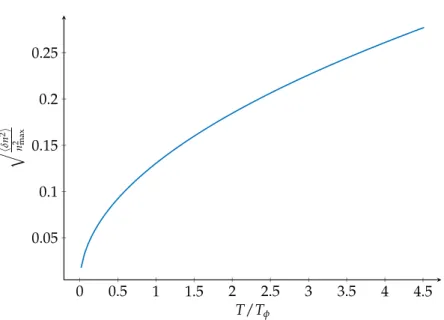
Averaging (δn�n0)2 over many realisations, the authors of [63] find an approximated relation for the mean square density fluctuations, at the centre of the trap, as a function of temperature: � �_�δn_n (0, t) 0(0, t) � � 2 � � _✏TT φ � log ⌧ ⇡ � � � � � �₁₊�₁_{+ �} �h!⊥⌧ µ log ⌧� 2 −√2� �. (2.49)

For ⌧→ 0, the mean square density fluctuations tends to �(δn�n0)2� → 0. For very long TOF, instead, the density fluctuations become bigger and bigger with �(δn�n0)2� ∝ √⌧. Eq. (2.49) has been proposed for thermometry of 1D gases, [63]. In Figure 2.4 we plotted the mean square density fluctuations as a function of T�µ for N = 2 ⋅ 104 atoms, !z= 2⇡ 4 Hz and !⊥= 2⇡ 400 Hz.

(24)

21 Elements of Bose-Einstein condensation 0 0.5 1 1.5 2 2.5 3 3.5 4 4.5 0.05 0.1 0.15 0.2 0.25 T/Tφ q hδ n 2i n 2 max

Figure 2.4.: Mean square density fluctuations as a function of T�Tφcomputed from (2.49) for N = 2 ⋅ 104 _{atoms, !}

z = 2⇡ 4 Hz and !⊥= 2⇡ 400 Hz and tTOF= 3 ms.

2.3. The spin-1 Bose Gas

Until now, we have discussed condensates with only one internal degree of freedom, also called scalar condensates. These were the first to be experimentally produced via evaporation in magnetic traps, [85, 31, 36]. When optical dipole traps became an accessible technology [170], it became easier to trap atoms with different hyperfine states in the same trap. This opened the possibility to study systems in which the interactions between different hyperfine components enrich the panorama. Degenerate Bose gases with a spin degree of freedom are called spinor condensates and we refer the reader to [84, 169] for a general exposition of the subject.

We start this section introducing the atomic structure of the Sodium atoms. From their properties, we construct the spinor Hamiltonian of the system and we find the ground state of this Hamiltonian based on a mean-field approach.

2.3.1. Hyperfine structure of Na atoms

The fine and hyperfine structures of Na atoms are sketched in Figure 2.5. The fine structure is the result of the coupling between the electron angular momentum L and the electron spin S. We note the levels with the usual spectroscopic notation N2S+1LJ, where the total angular momentum J= L + S. In Figure 2.5, see [172], we can observe the ground state and the two first excited states. D1 and D2 are the name of the transitions between the ground state and the two excited states.

To obtain the hyperfine structure, the interaction between the total angular momentum J and the nuclear angular momentum I, where I = 3�2 for 23_{Na, is needed. At low}

(25)

32_S 1/2 mF= −1 mF= 0 mF= +1 F = 1 F = 2 32_P 3/2 F0= 3 F0 = 2 F0 = 1 F0 = 0 32_P 1/2 1.77 Ghz 16 MHz 34 MHz 58 MHz D2 589.158 nm D1

Figure 2.5.: Fine and hyperfine structure of the electronic ground state of a Na atom.

magnetic fields, the good quantum number is the total hyperfine angular momentum F = J + I. As we can see in Figure 2.5, the ground state splits into two states with F = 1 and F = 2. The hyperfine splitting is ∆Ehf s ≈ 1.77 GHz. The excited states 32_P

1�2 and 32P3�2 split in 2 and 4 hyperfine levels. Each hyperfine levels F can then be divided in 2F+ 1 Zeeman sublevels corresponding to the projection of the total angular momentum along the quantisation axis. These levels are degenerate for zero magnetic fields. In our experiment, we trap 23Na atoms in an optical trap in the F = 1 ground state and we study the system composed by the three Zeeman sublevels mF = −1, 0 and +1. Optical dipole traps allow us to create the spin-independent potential we use to trap sodium atoms in the three Zeeman sublevels of F = 1. The red detuned8 light of the laser induces an electric dipole moment. The interaction between the induced dipole moment and the electric field creates the trapping potential. In principle the atom polarisability is a rank-2 tensor that can be decomposed in a sum of three irreducible operators of rank 0, 1 and 2. The three terms produce, respectively, a scalar, a vector and a tensor light-shift, see [53]. In our case, if we use far red detuned, linear polarised light, only the scalar term is important and the potential is spin-independent, see [65].

2.3.2. Two-body scattering between Na atoms

We have already introduced interactions in the low energy limit in the first section of the chapter. The result was the definition of the pseudopotential (2.6) to describe

two-8

Dipole trap can be blue detuned. In that case the laser light produce a repulsive potential for the neutral atoms.

(26)

body scattering. In the case of a spinor condensate, however, we have to consider also interactions between atoms in different internal degrees of freedom. In our case, we want to describe the scattering between two 23_{Na atoms with S}= 1.

First of all, the interaction potential is generated from the Coulomb repulsion between the electrons, so that it is invariant by spin rotations. This is an approximation, since magnetic dipole-dipole interactions break this symmetry. We neglect this contribution here and we justify this choice later. Also an applied magnetic field break the rotational symmetry, but the longitudinal spin projection Sz along the field direction is still conserved. When two atoms with S = 1 collide, they combine their angular momenta in a total angular momentum S= 0, 1 or 2 with mS= −S, . . . , S. Due to the rotational symmetry in angular momentum space, S is conserved during the collision. Therefore, we define a new interaction potential ˆ V(r, r′) = δ(r − r′) ⊗ � S gSPˆS (2.50) where gS = 4⇡�h 2_a S

m is the analogue of (2.7) for the S scattering channel and ˆPS = ∑mS�S, mS� �S, mS� is the projection operator on the subspace with total angular mo-mentum S.

We are discussing scattering events in the s-wave limit, hence the spatial part of the wave function is symmetric. The23Na atoms are bosons, therefore, also the spin part of the wave function must be symmetric. This means that only the S= 0 and 2 collisional channels are allowed. Thanks to the following two relations9:

1= ˆP0+ ˆP2 (2.51)

ˆ

S1⋅ ˆS2= ˆP2− 2 ˆP0 (2.52)

we can rewrite the potential (2.50) in the form ˆ

V(r, r′) = δ(r − r′) @

@rr⊗(¯g1 + gs ˆ

S1⋅ ˆS2) (2.53)

where there are two new coupling constant for the spin dependent and spin independent interactions: ¯ g= gS=0+ 2gS=2 3 , (2.54) gs= gS=2− gS=0 2 , (2.55)

The scattering lengths for sodium atoms were measured in [93] combining Feshbach resonances and coupled-channels calculations. The authors found

¯

a= 2.8 nm, (2.56)

as= 98 pm, (2.57)

9

The second relation can be derived using the expression of the total spin of the pair: (S1+ S2)2 =

(27)

The positive sign of as means that the atoms minimise their energy anti-aligning their spins. Therefore, the23_{Na Bose gas exhibits an antiferromagnetic behaviour.}

The ratio between the spin independent and spin dependent interaction is small: as

¯

a ≈ 0.036. (2.58)

It is interesting to give also the ratio between magnetic dipole-dipole and spin dependent interactions. Considering two magnetic dipoles µ1 and µ2, the interaction energy between two permanent dipoles is equal to

Udd= µ0 4⇡r3 �� (µ1⋅ µ2) − 3 r2(µ1⋅ r)(µ2⋅ r) �� (2.59)

where µ0 is the vacuum permeability and, for atomic magnetic dipoles, we can write µi= µBgjJi, where gjis the Landé factor and Jiis the total angular momentum. Therefore, for a polarised cloud with � �S� � = 1, the ratio between spin and dipole-dipole interactions is gdd gs ≈ µ0µ2Bm 16⇡�h2_a s ≈ 0.075 (2.60) From (2.60) it is clear that spin dependent interactions are much stronger than dipole-dipole interactions for 23Na atoms therefore we are allowed to neglect them. This approximation is not valid for atomic species with much higher magnetic moment as, for example, Chromium [178, 16], Dysprosium [97] and Erbium [2].

2.3.3. The Zeeman shift

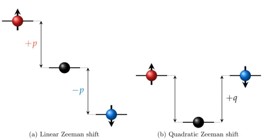
With interaction energy, another important energy scale for the system is provided by the magnetic field. Atoms are sensible to the application of an external magnetic field. In particular,23Na atoms have a magnetic dipole µ≈ µB�2. In the limit µBB�∆Ehf s� 1, where the total angular momentum F is a good quantum number, the effect of an external magnetic field on a single atom can be obtained via an expansion of the Breit-Rabi formula, see [172], ˆ H_mag(1)(F, mF) = (−1)F mFµBB 2 + (−1) F (µBB)2 4 ∆Ehf s�1 − m2_F 4 � + . . . (2.61) where ∆Ehf s is the hyperfine energy splitting. The first term of (2.61) is the linear Zeeman energy; as we can see in Figure 2.6, it shifts the mF = +1 and mF = −1 levels, with respect to the mF = 0 one, by +p and −p, respectively, where

p= µBB

2 ≈ h ⋅ 696 KHz

G ⋅ B (2.62)

The second term is the quadratic Zeeman energy, see Figure 2.6; it shifts both the mF = +1 and the mF = −1 levels, with respect to the mF = 0 one, by +q, where

q= (µBB) 2 4∆Ehf s ≈ h ⋅ 277 Hz G2 ⋅ B 2_. _(2.63)

(28)

+

p

−

p

(a) Linear Zeeman shift

+

q

(b) Quadratic Zeeman shift

Figure 2.6.: Effect of an external applied magnetic field on the Zeeman sub-levels of the F = 1 state of a23Na atom.

2.3.4. The Spinor Many-body Hamiltonian

The potential defined in (2.53) can be used to write the interaction many-body Hamiltonian for a systems of spin 1 bosons, see [169]:

ˆ Hint= ¯ g 2 � dr ˆn(r) 2₊gs 2 � dr ˆS 2 _(2.64)

where ˆn(r) is the number operator and ˆS = ( ˆSx, ˆSy, ˆSz) is the spin density operator. Using the explicit expressions for the three spin density operators

ˆ Sx= 1 √ 2�ˆΨ † +1Ψˆ0+ ˆΨ†₋₁Ψˆ0+ h.c.� (2.65) ˆ Sy= 1 √ 2� − iˆΨ † +1Ψˆ0+ iˆΨ†₋₁Ψˆ0+ h.c.� (2.66) ˆ Sz= ˆΨ†₊₁Ψˆ+1− ˆΨ†−1Ψˆ−1 (2.67)

and after some algebra, we can rewrite the interaction Hamiltonian as ˆ Hint= � dr�� ¯ g+ gs 2 Ψˆ † +1Ψˆ†+1Ψˆ+1Ψˆ+1+g₂¯Ψˆ†0Ψˆ † 0Ψˆ0Ψˆ0+ ¯ g+ gs 2 Ψˆ † −1Ψˆ † −1Ψˆ−1Ψˆ−1 + (g¯+ gs) 2 Ψˆ † +1Ψˆ†0Ψˆ+1Ψˆ0+ ( ¯ g+ gs) 2 Ψˆ † −1Ψˆ † 0Ψˆ−1Ψˆ0+ ( ¯ g− gs) 2 Ψˆ † 1Ψˆ † −1Ψˆ1Ψˆ−1 + gs�ˆΨ†₊₁Ψˆ†₋₁Ψˆ0Ψˆ0+ ˆΨ†₀Ψˆ†₀Ψˆ+1Ψˆ−1�� (2.68)

(29)

The first two lines of (2.68) give an energy shift due to the elastic collisions. The third line describes the only spin-flip collision allowed in the system. As we can see in Figure 2.7, two atoms in the Zeeman sub-levels mF = +1 and mF = −1 collide and come out as two atoms in the Zeeman sub-level mF = 0. Since the Hamiltonian, by construction, is invariant over rotation in the angular momentum space, the projection of ˆS along the quantisation axis must be conserved. This conserved quantity is the longitudinal magnetisation of the system

Mz = � dr ˆSz(r) = N+1− N−1 (2.69)

Until now we have considered only interactions. The term of the many-body Hamiltonian corresponding to the magnetic field effect , using p and q, can be rewritten as:

ˆ Hmag= p ˆSz− q� ˆN0+ 3 ˆN� (2.70)

+

1

−

1 0 0

Figure 2.7.: Inelastic collision permitted for a system of spin 1 bosons. Two atoms, in the Zeeman states mF = +1 and mF = −1 become two atoms in mF = 0. Since the Hamiltonian of the system is invariant over rotation in the total spin state, the projection of the total angular momentum along the quantisation axis, Mz= N+1− N−1, must be conserved in the scattering process.

2.3.5. Spinor BEC in the single spatial mode

We can now write the entire total many-body Hamiltonian ˆHtot = ˆHsp+ ˆHint+ ˆHmag, where ˆH_int comes from (2.68), ˆH_mag from (2.61) and

ˆ Hsp= � i � dr ˆΨ † i(r) �� − �h2_∆ 2m + ˆVext(r) �� Ψˆi(r) (2.71)

In this section, we want to find its ground state making a mean-field approxima-tion. This consists in choosing for all the atoms the same single-particle state φ(r) = �φ+1(r), φ0(r), φ−1(r)�. The mth component φm(r) of φ(r), is the condensate wave function of the spin component m. The many-body state of the system with all the atoms occupying the state φ can then be written as

�Ψ�N = 1 √ N!�a † φ� N �0� (2.72)

(30)

Table 2.1.: Coupling constants for the possible interactions between neutral atoms in the F = 1 manifold defined from the Hamiltonian (2.68).

2 ⋅ gAB mF = +1 mF = 0 mF = −1 mF = +1 g¯+ gs g¯+ gs g¯− gs

mF = 0 g¯+ gs g¯ g¯+ gs mF = −1 g¯− gs g¯+ gs g¯+ gs

To find the ground state of the Hamiltonian, we use the many-body state to compute the expectation value of G= �Htot� − µN. Minimising the resulting functionals over the φm’s, we obtain the three Gross-Pitaevskii equations for the three components wave functions φm(r): i�h@ @tφ+1= � �− �h2 2m∆+ Vext(r) + p � �φ+1+��g⇢¯ + gs�⇢0+ ⇢z�� φ+1+ gsN φ20φ∗−1 (2.73) i�h @ @tφ0= � �− �h2 2m∆+ Vext(r) − q � �φ0+� �g⇢¯ + gs�⇢+1+ ⇢−1�� φ0+ 2gsN φ+1φ−1φ∗0 (2.74) i�h@ @tφ−1= � �− �h2 2m∆+ Vext(r) − p � �φ−1+� �g⇢¯ + gs�⇢0− ⇢z�� φ−1+ gsN φ20φ∗+1 (2.75) where ⇢m(r) = �φm(r)�2 is the density of the spin component m and ⇢z= ⇢+1− ⇢−1 is the magnetisation density.

Another level of approximation, that is valid for our condensate in the 3D configuration, is based on the decoupling of the spatial and of the spin degrees of freedom by imposing, for the three components, the same spatial wave function. At first, we look at the miscibility and immiscibility of the different components of the spinor condensate. This will naturally bring us to introduce the Single Mode Approximation (SMA), which consists in the decoupling just described above.

Miscible and immiscible mixtures

Following the argument introduced in [168], we consider a mixture of two components in a box of volume V at T = 0. For simplicity, we restrict ourselves to a mixture of mF = +1 and mF = 0. Considering only the interaction energy of the condensed mixture,

E= 1 2�n

2

0g0+ n2₊₁g+1+ 2 n0n+1g0,+1�, (2.76) where the coupling constants for the different interactions are defined from the Hamiltonian (2.68), see Table 2.1. To understand if the two components overlap or if they phase separate, we have to compare the energies of the two configurations. We follow the work [6]. We

(31)

consider the two components to have the same number of atoms N. The two energies are: E_o= N

2

2V �g0+ g+1+ 2g0,+1�, (2.77)

for the overlapped case, and

Eps= N2 2 � g0 V0 + g₊₁ V₊₁�, (2.78)

for the phase separated case. In the latter case, the two volumes V0 and V+1 are defined minimising the energy Eps by varying V0 with V+1= V − V0. This corresponds to have equal pressure in the two phases:

g0� � N V0 � � 2 = g+1�_�_VN +1 � � 2 , (2.79)

so that they can be rewritten as V0= √_g 0g+1 g₊₁+ √g0g+1V and V+1= g₊₁ g₊₁+ √g0g+1V. (2.80) The energy for the phase separated case takes the form

E_ps= N 2

2V �g0+ g+1+ 2√g0g+1�, (2.81)

Comparing E0 and Eps, we find that the two components mF = +1 and mF = 0 phase separate if

g0,+1> √g0g+1. (2.82)

For Sodium atoms, from Table 2.1, ¯g+ gs > �

¯

g(¯g + gs): the condition is true and the components phase separate. Considering the different mixtures we can produce with the three components, we see that the mF = +1 and mF = −1 components are miscible and the mF = 0 component is not miscible with the other two.

The Single Mode Approximation

As we have just seen, the different components of the condensate separate and form domains in a trap. We focus now our attention on the 3D geometry; the 1D geometry is treated in details in Chapter 4. Making an analogy with the healing length (2.14), we can define the spin healing length

⇠s=

� �h2 2mgsn

(2.83) This is the length over which the spin wave function recover from a perturbation. If our condensate size is much smaller than this characteristic length ⇠s, it is not energetically favourable to form spin domains that would cost a tremendous amount of kinetic energy

(32)

29 Elements of Bose-Einstein condensation ∼ �h2

md2 � µ with d the domain size. Therefore, for atom clouds small enough, we can consider the three Zeeman components to have the same spatial wave function: this approximation is called Single Mode approximation (SMA).

In the Thomas-Fermi regime, the condensate size R is given by (2.12), so the condition for the validity of SMA R� ⇠s, can be written as

µ �h! � � ¯ g gs or gsn� � gs ¯ g �h! (2.84)

In the case of µ∼ �h! the condensate size is R ∼�_m!�h and from the condition R� ⇠s we obtain

gsn� �h! (2.85)

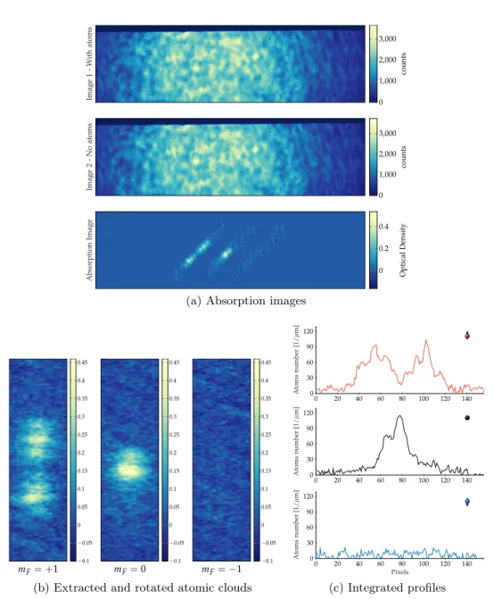
These expressions set an upper limit on the number of atoms for the SMA approximation to hold. As we will see in Chapter 5, this condition can be valid along some trap axes and fails along others. For our system in the 3D trap, where densities are on the order n = 1014cm−3, the spin healing length ⇠s ∼ 1 µm, which is of the same order of the condensate length. Therefore, the SMA is a good approximation for our 3D system. For a more involved discussion about the validity of this approximation in our system, we refer the reader to [32]. In Figure 2.8, we can see an image of the three components after time of flight in a magnetic field gradient. The profiles, obtained integrating the optical density along a CCD axis, can be nicely fitted by three Thomas-Fermi distributions with the same radii.

Introducing the SMA approximation, we write the condensate wave function as

�φ(r)� = φ(r) ⊗ �⇠� (2.86)

where the spatial wave function φ(r) is frozen and can be used to minimise G = �H�−µN, where we consider only the Hamiltonian Hsp plus the first term of the interaction Hamiltonian (2.64) to obtain the Gross-Pitaesvkii equation

� �− �h2 2m∆+ Vext(r) + ¯gN�φ(r)� 2_φ_(r)� �φ(r) = µφ(r), (2.87)

We can parametrise the spin wave function in the following way, see [169]:

�⇠� =�� √_n +1ei✓+1 √_n 0ei✓0 √_n −1ei✓−1 � � �= e i✓0 � �� x+mz 2 e i(Θ+↵) 2 √ 1 − x �_x−mz 2 e i(Θ−↵)₂ � �� (2.88)

where we introduce the reduced quantities nm=

Nm

(33)

R OD

x

Figure 2.8.: Image of the three components after time of flight. The three profiles, obtained by integration of the optical density along one CCD axis, are well fitted by three Thomas-Fermi profiles with the same radii.

and the two relatives phases

Θ= ✓₊₁+ ✓−1− 2✓0 and ↵= ✓+1− ✓−1. (2.90) We can use it to minimise the Hamiltonian ˆHtot = g₂s∫ dr ˆS2+ ˆHmag and obtain a spin energy Espin= Us 2N �ˆS� 2 − q ˆN0, (2.91) where Us= Ngs� dr �φ(r)�4, (2.92)

is the spin interaction energy. For 23Na, gs > 0 and so also the interaction energy is positive. In the Hamiltonian there is no linear Zeeman energy. The latter is proportional to the longitudinal magnetisation mz, which has a fixed value and it is a conserved quantity. Therefore, it only gives a constant shift of the energy that has been omitted. Only the quadratic Zeeman energy contributes to the spin dynamics of the system. The equilibrium phase diagram

From the spin wavefunction (2.88) and the spin energy (2.91) we obtain an energy functional that can be minimised to find the system ground state:

E_spin=N Us 2 �m 2 z+ 2x(1 − x) + 2 cos(Θ)(1 − x) √ x2_{− mz}2� + NU sqx. (2.93)

(34)

All the different states are degenerate with respect to the relative phase ↵. Since Us> 0, to minimise the energy the other phase Θ locks to Θ= ⇡, independently of the value of x and mz. This locking of the relative phase enforces the presence of a nematic order in the system, as we experimentally demonstrated in [196].

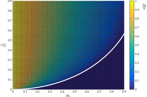
The energy functional (2.93) can be minimised by varying the parameter x, with mz and q imposed experimentally. The result is represented in Figure 2.9: a second-order phase transition appears as the magnetic field grows . This has been studied experimentally in [76].

For mz= 0 and q > 0, we obtain a state with energy Espin= NUsqx. The energy minimum is at x= 0, i.e. the state is characterised by all the atoms in mF = 0. In the case q = 0 we find a family of states called polar states�Ω� introduced in [65]. They can be written as:

�Ω� = R(✓, φ) ⋅�� 0 1 0 � � �= � �� − 1 √ 2sin(✓) e −iφ cos(✓) 1 √ 2sin(✓) e iφ � �� (2.94)

These are states for which all atoms are in the mF = 0 state with respect to a quantisation axis n, defined by the polar angles(✓, φ), and are all degenerate. A full quantum treatment of the case mz= 0 and q = 0 can be found in [101].

Looking at the energy functional at mz> 0, we can rewrite it as Espin

N = Us(1 − x)�x − �

x2_{− m}2

z� + qx (2.95)

There are two contributions to the energy: i.) the interactions, presented in Figure 2.7, tend to minimise the energy locking x= 1; this is what we expect from an antiferromagnetic system as our gas of sodium atoms; ii.) the magnetic field, on the contrary, with the quadratic term q, tries to reduce the energy transfering as many atoms as it is possible10 in mF = 0. These two effects compete to determine the system equilibrium state. Looking at Figure 2.9, we see that, for each magnetisation, there is a critical value of q dividing the equilibrium phase diagram in two regions. This critical value is equal to

qc= Us(1 − �

1 − m2

z) (2.96)

and it is sketched with a white line in the Figure.

For q< qc, the magnetic field is not high enough to overcome the effect of the interactions and the ground state of the system is antiferromagnetic, with n_±1= (1 ± mz)�2 and n0= 0. We call this state also quasi-spin nematic (qSN) state. Increasing the magnetic field, it is more and more energetically favourable for the system to transfer atoms in mF = 0. For q> qc, n0 starts to grows with q until a maximum value fixed by the conservation of the magnetisation mz = n+1. We call this ground state transverse magnetised (M⊥).

10

The magnetisation is fixed, so there is a maximum number of atoms that can be transferred to the mF = 0 state from mF= +1 and mF = −1.

(35)

N0 N 0 0.1 0.2 0.3 0.4 0.5 0.6 0.7 0.8 0.9 0 0.1 0.2 0.3 0.4 0.5 0.6 0.7 0.8 0.9 mz q _Us 0 0.1 0.2 0.3 0.4 0.5 0.6 0.7 0.8 0.9 1

Figure 2.9.: Equilibrium phase diagram for a condensate of 23Na atoms. The two axes correspond to the longitudinal magnetisation mz and to the ratio between the quadratic Zeeman term and the interaction energy _Uq

s. The color scale represents the population in the Zeeman state mF = 0. The white line divides the diagram into two regions: for small magnetic fields, the system is in the antiferromagnetic state, with n_±1 = (1 ± mz)�2 and n0 = 0. For high magnetic fields, the system is in the transverse magnetised (M_⊥) phase, where mF = 0 becomes populated. Due to the conservation of the longitudinal magnetisation, there is a maximum number of atoms that can be transferred in this state.

(36)

3. Production and characterization of a

spin-1 Bose-Einstein condensate of

Sodium atoms

In this Chapter, we present in Section 3.1 and Section 3.5 the experimental recipe used to produce the 3D and the 1D condensate and to probe them. We present also in Section 3.2 the techniques used to manipulate the spin internal degrees of freedom of the spinor condensate.

The description of the experimental apparatus is reduced to the main parts needed to understand the experimental recipe. We refer the reader to the PhD Thesis [75, 118] for a comprehensive description of all the components.

3.1. Experimental Setup and cooling techniques

This section is devoted to the description of the experimental apparatus and the experi-mental sequence we use to reach quantum degeneracy from a dilute thermal gas of bosonic 23_{Na atoms and obtain a Bose-Einstein condensate.}

3.1.1. UHV chamber and atomic source

Spinor gases are very fragile with respect to stray magnetic fields [66, 8] and this is why our ultra high vacuum (UHV) chamber is made of Titanium, which has a low magnetic susceptibility. A schematic of the vacuum chamber is sketched in Figure 3.1.

All cold atoms experiments require an atom source, a magneto-optical trap (MOT) to collect hot atoms directly from this source and a second trap, where atoms can be cooled down to the quantum degeneracy by evaporation cooling techniques, see [86].

An efficient loading of the MOT requires an high background pressure, while the evap-orative cooling of the trapped cloud requires UHV: the collisions between the trapped atoms and atoms of the background vapour can severely affect the evaporation process. These two opposite requirements are then matched using a dispenser as atomic source and light-induced atomic desorption (LIAD) to control the background pressure, see [119].

(37)