HAL Id: tel-01222160
https://tel.archives-ouvertes.fr/tel-01222160
Submitted on 29 Oct 2015
HAL is a multi-disciplinary open access archive for the deposit and dissemination of sci-entific research documents, whether they are pub-lished or not. The documents may come from teaching and research institutions in France or abroad, or from public or private research centers.
L’archive ouverte pluridisciplinaire HAL, est destinée au dépôt et à la diffusion de documents scientifiques de niveau recherche, publiés ou non, émanant des établissements d’enseignement et de recherche français ou étrangers, des laboratoires publics ou privés.
elimination and nitrification in a new multi-section
bioreactor
Haoran Pang
To cite this version:
Haoran Pang. Study of the hydrodynamic characteristics, COD elimination and nitrification in a new multi-section bioreactor. Fluids mechanics [physics.class-ph]. INSA de Toulouse, 2014. English. �NNT : 2014ISAT0003�. �tel-01222160�
Study of the hydrodynamic characteristics, COD
elimination and nitrification in a new
Multi-section Bioreactor
Thesis submitted to the
National Institute of Applied Science, Toulouse for award of the degree
of
Doctor of Environmental Engineering
By
Haoran PANG
L'objectif principal de ce travail de thèse concerne l'étude de l' élimination de la DCO et de la nitrification dans une nouveau lit bactérien Multi-Section ( MSB ) . Après une caractérisation de l’hydrodynamique et du transfert d’oxygène de ce lit bactérien, les expériences biologiques menées sous des conditions opératoires contrastées (fortes et faibles charges organiques et eaux usées contenant ou pas des matières particulairs) ont été menées. En parallèle, des simulations avec le logiciel Biowin ont été réalisées. Les principaux résultats sont résumés en suivant :
- La rétention de liquide statique est majoritaire par rapport à la rétention dynamique que ce soit en présence ou en absence de biofilm. Le biofilm joue le rôle d’une "éponge" permettant un maintien de l’humidité du lit même à faible débit. Les expériences de DTS ont montré que le biofilm accroit le temps de séjour du liquide et conduit à une diminution de l’épaisseur du film liquide permettant ainsi de promouvoir le transfert de l'oxygène. - Le réacteur MSB montre une élimination efficace de la DCO (> 95 % ) et de la nitrification ( > 60 % de l’azote entrant), mais une accumulation de DCO particulaire a lieu dans le filtre ce qui conduira à un colmatage à terme. La nitrification cohabite avec l’élimination de la DCO même dans la première section et pour une charge organique élevée ce qui implique une bonne capacité d’oxygénation du MSB par l’aération naturelle. - Un modèle dynamique de MSB a été utilisé implémenté sur le simulateur - BioWin , afin d'obtenir la répartition des biomasses au sein du réacteur et d'évaluer le processus limitant dans chaque section. Le modèle partiellement calibré peut aider à estimer les besoins minimum d'oxygène pour la nitrification et peut rendre compte de la compétition entre la croissance hétérotrophe et la nitrification.
Mots-Clés:
Traitement décentralisé des eaux usées, lit bactérien, hydrodynamique, distribution des temps de séjour (DTS), épaisseur de film liquide, transfert d'oxygène, nitrification, élimination de l’azote, simulation
The main objective of this PhD work focused on the study of the COD removal and nitrification in a new designed Multi-Section Bioreactor (MSB). Hydrodynamic characterization of the reactor, biological experiments under contrasted conditions and simulations by Biowin software were carried out:
- Firstly, it was found that static liquid retention is the predominant part both without and with the presence of biofilm. Biofilm acts like a "sponge". RTD experiments showed that biofilm can promote liquid residence time, decrease the liquid film and promote the oxygen transfer consequently.
- Secondly, the MSB operated at contrasted organic loading rate (OLRs) and nitrogen loading rate (NLRs) showed that COD can be effectively removed (removal efficiency > 95%) and nitrification (> 60% of the N removal) occurred in this biofilter. Nitrification is efficient even in the first section implying no drastic oxygen limitation though only natural aeration is occurring.
- Thirdly, a TF dynamic model has been used from a simulator - BioWin, in order to get more insights on the biomass distribution in the pilot and to assess the limiting process in each section of the bioreactor. Calibration of the model can help us to estimate the minimum oxygen requirement for nitrification for each zone inside the pilot and it can well represent the competition between heterotrophic growth and nitrification.
Key words:
Decentralized wastewater treatment, trickling filter, hydrodynamic, residence time distribution (RTD), oxygen transfer, nitrification, nitrogen removal, simulation, Biowin software
Acknowledgement
I would like to express my deep and sincere gratitude to my Supervisors Prof. Etienne PAUL and Prof. Valerie LETISSE for their valuable guidance, inspiration, constant encouragement and heartfelt good wishes. Their genuine interest in the research topics, free accessibility for discussion sessions, thoughtful and timely suggestions has been the key source of inspiration for this work. I feel indebted to both my supervisors for giving abundant freedom to me for pursuing new ideas. It was overall a great experience of working with both of them.
I record my sincere thanks and gratitude to Prof. Gilles HEBRARD, for his cordial advice and suggestions on hydrodynamic experiments and simulations, and continued encouragement throughout all this work. Not to mention those valuable guidance, inspiration, constant encouragement and heartfelt good wishes for my publications and for the presentations during my works.
My special thanks to my colleagues Mañas Angela., Irene Mozo., Yoan Pechaud, Matthieu Peyrela for their help in performing various experiments and modeling work.
I express my special thanks to my friend Chengcheng LI for his readiness to help for anything and everything for the current work.
I remain ever grateful to our technical staffs Mr. Mansour Bounouba and Mr. Evrard Mengelle for their assistance in experimental work.
Finally, I would like to thank my family in China, for their patience and support for this thesis, I owe them so much. The thesis would remain incomplete without mentioning the contributions of my parents for making me what I am today.
Greek letter
φcb: Apparent packing-bed void fraction (-)
ε: Total packed bed void fraction (-)
ε’ : Particle porosity (-)
dp: Equivalent sphere diameter (cm)
Φ: Sphericity of particle (-)
σ: Liquid surface tension (N·m-1)
σ²: Variance of calculated RTD from experimental RTD (-)
ρL: Liquid density (kg·m
-3 )
ρparticle: Particle density (kg·m
-3 ) α: Contact angle between the liquid and solid sphere (°)
δL: Liquid film thickness (mm)
βd: Liquid dynamic retention (dynamic volume/pure solid volume) (-) βs: Liquid static retention (static volume/pure solid volume) (-) βt: Total liquid retention (total liquid volume/pure solid volume) (-)
τ: Theoretical liquid residence time (s)
τH: Hydraulic residence time (s)
τp: Shear stress (Pa)
μ: Mean liquid residence time from RTD curves (s) μmax: Maximum specific heterotrophic/autotrophic growth rate (d
-1 ) μH: Specific heterotrophic growth rate (d
-1 ) μA: Specific autotrophic growth rate (d
-1 )
θ: Dimensionless time (-)
ν : Kinematic viscosity (m2/s)
θd: Sludge retention time (d)
Latin letter
bH: Heterotrophic decay rate (d
-1 )
bA: Autotrophic decay rate (d
-1 )
hLt: Total liquid holdup (m
3 )
hLS: Liquid static holdup (m
3 )
hLd: Liquid dynamic holdup (m
3 )
hlpore: Pore holdup (-)
hlcap: Capillary rise holdup (-)
hlres: Residual holdup (-)
hcap: Liquid capillary rise height (m) hin.cap: Internal capillary rise height of single particle (m) hex.cap: External capillary rise height of single particle (m) min.cap: Liquid internal capillary mass of the packed bed (kg) mex.cap: Liquid external capillary mass of the packed bed (kg)
hcb: Height of packed bed (m)
mDP: Total dry packing mass (kg)
mLS: Liquid static holdup mass (kg)
mfd: Fast dynamic holdup mass (m
3 )
msd: Slow dynamic holdup mass (m3)
VLS: Liquid static holdup volume (m)
VLd: Liquid dynamic holdup volume (m
3 )
Vsolid: Pure solid volume (m
3 ) Vp,L: Liquid volume around single particle (m
3 ) Veffective: Effective liquid volume involved in RTD curves (m3)
Nparticles: Number of particles (-)
m: Fraction of active zone in packed bed (-) fW Wetting fraction of the packed bed (-) fLSE Fraction of partial static holdup volume of tracer exchange (%)
Lf: Biofilm thickness (mm)
Sh: Sherwood number (-)
Re: Reynolds number (-)
Sc: Schmidt number (-)
S Soluble substrate concentration (g/m³)
X: Biomass concentration (g/m³)
Ks: Substrate half-saturation coefficient (g/m³) bH: Decay rate of heterotrophic biomass (d
-1 )
KH: Hydrolysis rate (d
-1 ) KS: Carbon substrate half saturation coefficient (gCOD/m³) KO: Oxygen half saturation coefficient (gO2/m³) KNH: Ammonia half saturation coefficient (gN/m³)
Ds : Mass diffusivity coeffecient (m2/s)
DO : Oxygen diffusivity coeffecient (m
2 /s) DNH : Ammonia diffusivity coeffecient (m
2 /s)
Su Soluble inert organics (mg/L)
SB Readily biodegradable substrate (mg/L)
Xu Particulate inert organics (mg/L)
XB Slowly biodegradable substrate (mg/L)
Xoho Active heterotrophic biomass (mg/L)
Xba Active autotrophic biomass (mg/L)
Xu,e Unbiodegradable particulates from cell decay (mg/L)
Xsto Cell internal storage product (mg/L)
ISS Cell internal storage product (mg/L)
So Dissolved oxygen (gO2/m³)
Sno Nitrate and nitrite N (gN/m³)
Snh Free and ionized ammonia (gN/m³)
Snd Soluble biodegradable organic nitrogen (in SB) (gN/m³) Xnd Particulate biodegradable organic nitrogen (in XB) (gN/m³)
Snn Dinitrogen (gN/m³)
salk Alkalinity (mole/m³)
Xii Inert inorganic suspended solids (g/m³) YH: Heterotrophic yield coefficient -
YA: Autotrophic yield coefficient (gCOD/gN)
Abbreviation
P.E.: Per Equivalent
SA: Total surface area of packed bed (m2)
SSA: Specific surface area (m2/m³)
SAeff: Effective surface area of packed bed (m
2 )
S.H.L: Surface hydraulic loads (m·h-1)
HLR: Hydraulic loading rate (m·h-1)
OLR: Organic loading rate (m·h-1)
OUR: Oxygen Uptake Rate (mgO/L/h)
WWTP: Waste Water Treatment Plant
CWWTP Central Waste Water Treatment Plant
OWTS: On-site Wastewater Treatment System
STEP: Septic Tank Effluent Pumping System
SP: Stabilization Ponds
SBR: Sequence Batch Reactor
BFR: Biofilm Fluidized Bed reactors
UASB: Upflow Anaerobic Sludge Blanket reactor
BASR: Biofilm Airlift Suspension Reactor
AS: Activated Sludge TF: Trickling Filter
TFC: Trickling Fixed-bed Column
MSB: Multi-Section Bioreactor
RTD: Residence Times Distribution
PF: Plug Flow
CSTR: Continuous Stirred-Tank Reactor
HRT: Hydraulic Retention Time (h or s)
LRT: Liquid Residence Time (h or s)
SRT: Sludge Retention Time (d or h)
COD: Chemical Oxygen Demand
CODt: Total COD
CODs: Soluble COD
CODp: Particulate COD
BOD: Biological Oxygen Demand
BOM: Biological Organic Matter
EPS: Extracellular Polymeric Substances
TKN: Total Kjeldahl Nitrogen
TKNt: Total Kjeldahl Nitrogen
TKNs: Soluble Kjeldahl Nitrogen
N-NOx: Nitrite and nitrate nitrogen
OHO: Ordinary Heterotrophic Organisms
AOB: Ammonia Oxidizing Biomass
Figure I- 1: Recommended and possible domain of utilization of different types of wastewater treatment plants ... 3
Figure I- 2:Concentration- flow rate phase diagram for application of flocs and biofilm bioreactors ... 4
Figure I- 3: Diagram of a conventional Trickling filter ... 5
Figure I- 4: Schematic representation of the different processes and different morph-types of bacterial aggregates.. ... 7
Figure I- 5: Consumption of biodegradable COD ... 8
Figure I- 6: Removal of ammonia ... 9
Figure I- 7: Diagram of mass balance in the pilot ... 10
Figure I- 8: Conceptual profile of a fixed biofilm ... 15
Table I- 2: Summary of significant relationships between the numbers of Sherwood (Sh) or Reynolds (Re) and Schmidt (Sc), ε (porosity of the fluidized bed), d (pipe diameter), L (length of pipe) n1, n2, m (experimental constants). ... 18
Table I- 3: Models of detachment in literatures ... 19
Table I- 4: Biofilm density and fd in literatures ... 21
Figure I- 9: Schematic diagram of general mechanisms in a biofilm system ... 22
Table I- 5: Elements affecting the performance of nitrifying biofilms on a biofilm oriented and a reactor specific level ... 23
Table I- 6: TF classification from EPA criteria ... 24
Table I- 7: Typical OLR for single-stage nitrification ... 26
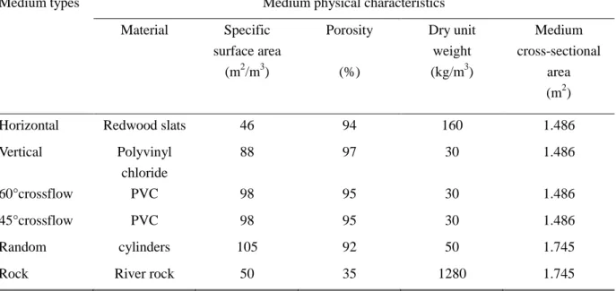
Figure I- 10: Typical Medium employed in Trickling Filter ... 28
Table I- 8: Filter Medium characteristics in research of Harrison and Daigger, (1987)... 28
Figure I- 11: Diagram of the theoretical relation between contact time and flow ... 29
Figure I- 12: Comparison of different media accounting for relations of filter depth and hydraulic loads with BOD removal efficiency based on modified Velz equation. ... 31
Figure I- 13: Medium configuration effect on nitrification versus volumetric organic loads ... 31
Figure I- 14: Conceptual diagram of the TF model ... 38
Table I - 1: Pollutants composition of a typical rural wastewater comparing with wastewater from a CWWTP in China ... 42
Table I- 9: Relation between non-biodegradable COD fractions and BOD5/COD ratio ... 44
Figure I- 15: Comparison of biodegradability of several decentralized wastewater ... 44
Table I- 10: Household water consumption and accordingly wastewater discharge (per capita) in rural areas in different countries/areas ... 45
Figure I- 16: Rural wastewater diurnal flow and components concentrations variation ... 46
Figure I- 17: Total variation coefficient with respect to the daily flowrate ... 47
Table I- 11: Comparison between the typical municipal and rural wastewater in terms of their daily flow, COD loads, TAN loads and variation of daily flow ... 48
Figure II- 1: Diagram of TFC (a) and MSB (b) ... 53
Table II- 1: Geometrical characteristics of the TFC and the MSB ... 53
Table II- 2: Composition of feed wastewater for two cultivated organic loads ... 54
Figure II- 2: Liquid holdup fractions in literatures (a) (b) and in this study (c) ... 58
Figure II- 3: Schematic of liquid layer and contact surface ... 61
Figure II- 4: Schematic of oxygen transfer ... 62
Table II- 3: Composition of wastewater fed for two regimes of organic loads cultivation ... 64
Figure II- 9: Schematic diagram of the TF and MSB system ... 75
Table II- 5: Input operating conditions ... 76
Table II- 6: Physical properties of TFC and MSB ... 76
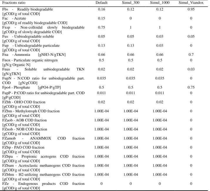
Table II- 7: Fractions ratio adjustments to fit the biological influent components ... 77
Table II- 8: Components in the influent ... 78
Table II- 9: Default and current values of kinetic parameters ... 78
Table II- 10: Aeration equipment parameters ... 79
Figure II- 10: Oxygen modeling operations ... 80
Figure II- 11: Biowin album for data output... 81
Figure II- 12: Start to simulate considering the data check and simulate under steady-state ... 81
Figure II- 13: Generate a simulation report to Word ... 82
Table III-1: Physical properties of Concrete block media and packed bed ... 84
Figure III- 1: Relation between number of particles and liquid static hold-up fraction. ... 85
Figure III- 2: Static hold-up volume versus number of particles. ... 86
Table III-2: Internal and external capillary rise height, capillary holdup and mass ... 87
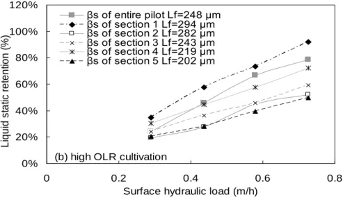
Figure III- 3: Liquid static retention of each section (section 1 is located at the top) and the entire pilot under different hydraulic conditions ... 89
Figure III- 4: Dynamic holdup release process curve for a flowrate of 0.3 m3/h in TFC ... 90
Table III- 3: Results of Holdup mass from two bioreactors’ experiments ... 91
Figure III-5: Liquid retention versus surface hydraulic loads in two bioreactors without biofilm ... 92
Figure III-6: Liquid dynamic retention versus surface hydraulic load for the MSB reactor in presence of biofilm. ... 93
Table III- 4: Dynamic model results from literatures and in this study ... 94
Figure III- 7: Conductivity versus time at different flow rates in MSB. ... 96
Figure III- 8: Volume of liquid represented in RTD determination ... 97
Table III- 5: Effective liquid volume Veffective calculated based on mean liquid residence time μ and flowrate Q, compared to the dynamic liquid volume VLd by drainage ... 97
Figure III- 9: Dimensionless RTD curves with thick biofilm and without biofilm at different surface hydraulic load in two reactors ... 99
Figure III- 10: RTD curve with/without biofilm at flow rate of 0.0091 m3/h in MSB ... 100
Figure III- 11: Calculated RTD curves based on three models and experimental RTD for the cases without and with biofilm at a flow rate of 9.1 L/h ... 102
Table III- 6: General results comparison of 3 different models ... 102
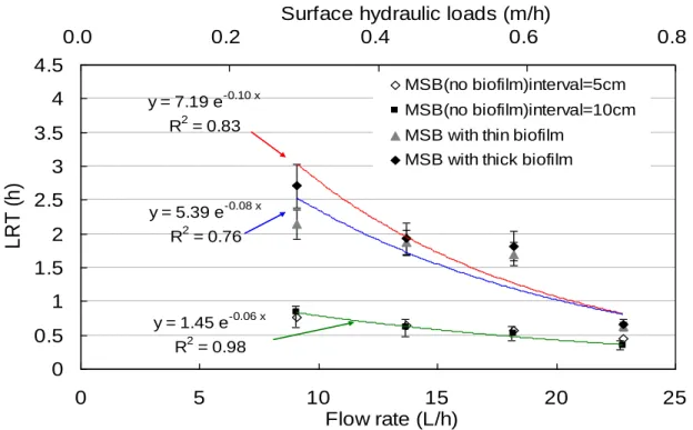
Figure III- 12: Calculated LRT based on RTD under different flow rates ... 104
Figure III- 13: Liquid film thickness versus hydraulic loads of regimes with/without biofilm ... 106
Figure III- 14: Volumetric oxygen transfer coefficient under different flowrates in cases without and with biofilm ... 107
Table III- 7: kLa from literatures and estimated in this study ... 108
Figure IV- 1: COD removal, nitrogen removal and nitrification yield on time course ... 111
Table IV- 1: Operating conditions during the three periods 2-4. ... 111
Table IV- 2: COD removal efficiency in period 2-4. ... 112
Figure IV- 2: CODt inlet and CODs outlet from the first section. Period 2 Low loading condition, water from diluted real WW ...113
Figure IV- 3: CODt inlet and CODs outlet from the first section. Period 3 high loading condition, water from diluted real WW ...114
water from diluted real WW ...115
Figure IV- 6: Soluble COD time-evolution concentration variation in section 2 to section 4. Period 3 high loading condition, water from diluted real WW ...115
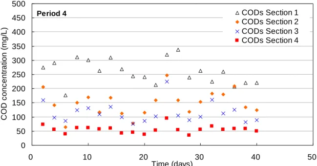
Figure IV- 7: Soluble COD time-evolution concentration variation in section 2 to section 4. Period 4, high loading condition, Viandox ...116
Figure IV- 8: Time-evolution of CODp at the outlet of section 1. Period 2, low loading condition, real WW ... 117
Figure IV- 9: Time-evolution of CODp at the outlet of section 1. Period 3, high loading condition, real WW ... 118
Figure IV- 10: Time-evolution of CODp at the outlet of section 1. Period 4, high loading condition, Viandox ... 118
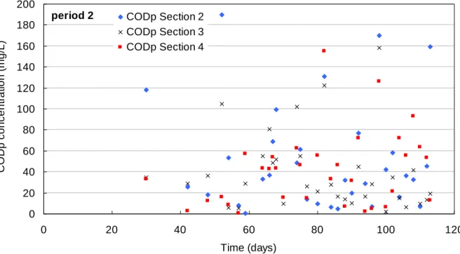
Figure IV- 11: Time-evolution of CODp concentration in section 2-section 4. Period 2, low loading condition, real WW .... 119
Figure IV- 12: Time-evolution of CODp concentration in section 2-section 4. Period 3, high loading condition, real WW ... 119
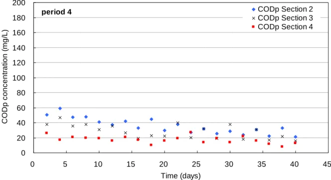
Figure IV- 13: Time-evolution of CODp concentration in section 2-section 4. Period 4, high loading condition, Viandox ... 120
Figure IV- 14: CODt and CODs along the filter. Period 2, low loading condition, real WW ... 121
Figure IV- 15: CODt and CODs along the filter. Period 3, high loading condition, real WW ... 122
Figure IV- 16: CODt and CODs along the filter. Period 4, high loading condition, Viandox ... 122
Figure IV- 17: Photos of section 1 at the end of each period ... 123
Table IV- 3: Removal efficiency of a full-scale unit in comparison with literature ... 124
Figure IV- 18: Total COD removal in a full-scale demonstration unit in China ... 125
Figure IV- 19: Pathways of total COD ... 126
Figure IV- 20: Relation between consumed COD and nitrogen assimilation. Period 4, high loading condition, Viandox ... 128
Table IV- 4: TKN removal and nitrification performance ... 131
Figure IV- 21: TKN time-evolution concentration in each section. Period 2, low loading condition, real WW ... 132
Figure IV- 22: TKN time-evolution concentration in each section. Period 3, high loading condition, real WW... 132
Figure IV- 23: TKN time-evolution concentration in each section. Period 4, high loading condition, Viandox... 133
Figure IV- 24: Nitrate and nitrite time-evolution concentration in each section. Period 2, low loading condition, real WW . 134 Figure IV- 25: Nitrate and nitrite time-evolution concentration in each section. Period 3, high loading condition, real WW 134 Figure IV- 26: Nitrate and nitrite time-evolution concentration in each section. Period 4, high loading condition, Viandox. 135 Figure IV- 27: Nitrate and nitrite time-evolution concentration in section 1. Period 2 to 4 ... 136
Figure IV- 28: Calculated TKN consumed, nitrate produced and ammonia consumed for each period of time. Period 2, low loading condition, real WW. ... 137
Figure IV- 29: Calculated TKN consumed, nitrate produced and ammonia consumed for each period of time. Period 3, high loading, real WW ... 137
Figure IV- 30: Calculated TKN consumed, nitrate produced and ammonia consumed for each period of time. Period 4, high loading, Viandox ... 138
Table IV- 5: Removal efficiency of a full-scale unit in comparison with literature ... 139
Figure IV- 31: TN and ammonia removal in full-scale reactor ... 140
Figure IV- 32: Pathways of nitrogen ... 141
Table IV- 6: Biofilm thickness estimation by optical method ... 145
Figure IV- 36: LRT estimation during period 2-period 4. ... 146
Figure IV- 37: Liquid film thickness estimation during period 2 to period 4. ... 147
Figure IV- 38: Schematic diagram of biofilm and liquid film during period 2 to period 4. ... 148
CHAPTER 1-BIBLIOGRAPHY
PART 1: TREATMENT SYSTEMS USED FOR MACRO-POLLUTANTS REMOVAL IN
DECENTRALIZED AREA ... 1
1. OVERVIEW OF TREATMENT TECHNIQUES ... 1
1.1 Technologies for rural wastewater treatment ... 1
1.2 Attached growth & Suspended growth systems ... 3
2. OVERVIEW OF TRICKLING FILTER PROCESS ... 5
2.1 Single-stage TF ... 5
2.2 General Principal in TF ... 6
PART 2: DESCRIPTION OF A BIOFILM AND OF BIOLOGICAL PROCESSES ... 7
1. BRIEF OF BIOFILM ... 7
2. BIOLOGICAL REACTIONS ... 8
2.1 Principal of COD removal ... 8
2.2 Principal of nitrification ... 8
3. BIO-KINETICS OF MODELING A BIOFILM SYSTEM ... 10
3.1 Mass balance kinetic of overall system ... 10
3.2 Mass transformation kinetics ... 11
PART 3: DESCRIPTION OF PHYSICAL PROCESSES ... 15
1. PHYSICAL PROCESSES... 15
1.1 Mechanisms of mass transfer and transport ... 15
1.1.1 External mass transfer ... 15
1.1.2 Internal mass transport ... 20
2. PARTIAL CONCLUSION ... 23
PART 4: PILOT DESIGN ... 24
1. DESIGN CRITERIA ... 24
1.1 For COD removal ... 24
1.2 For nitrification ... 26
1.3 Competition between heterotrophs and autotrophs in biofilm systems ... 26
2. MEDIUM SELECTION... 27
2.1 Types of medium ... 27
2.2 Performance based on Medium configuration ... 29
3. DIMENSIONING A PILOT ... 32
3.1 Particular consideration of new structure ... 32
3.2 Dimensioning our pilot for lab-scale experiments ... 33
4. PARTIAL CONCLUSION ... 33
PART 5: MODELING OF TF ... 35
1. INTRODUCTION OF THE SOFTWARE BIOWIN ... 35
1.1BioWin in Brief ... 35
1.2 TF Module ... 36
1.2.1 Conceptual model of TF ... 37
1. INTRODUCTION ... 42
2. CHARACTERISTICS OF RURAL WASTEWATER ... 42
2.1 Rural wastewater quality ... 42
2.2 Treatability of rural wastewater ... 43
3. RURAL WASTEWATER FLOW ... 45
3.1 Daily discharge of rural wastewater ... 45
3.2 Hourly flow and components’ concentrations variation ... 46
4. PARTIAL CONCLUSION ... 48
CHAPTER 2 - MATERIAL AND METHODS PART 1: MEDIUM AND BIOREACTOR CHARACTERIZATION AND HYDRODYNAMIC BEHAVIOR INVESTIGATION ... 52
1. OBJECTIVES ... 52
1.1 Experimental System ... 52
1.2 Methods ... 54
1.2.1 Particle Diameter and Density ... 54
1.2.2 Static hold-up measurements ... 55
1.2.3 Static hold-up model ... 56
1.2.4 Dynamic hold-up measurements ... 57
1.2.5 Residence Time Distribution (RTD) ... 58
1.2.6 RTD models ... 59
1.2.7 Liquid film thickness estimation ... 61
1.2.8 Volumetric oxygen transfer coefficient kLa estimation ... 62
PART 2: BIOLOGICAL EXPERIMENTS ... 64
1. INTRODUCTION ... 64
2. MATERIAL AND METHODS ... 64
2.1 Feeding conditions ... 64
2.2 Methods ... 65
2.2.1 Sifting method for primary sludge... 65
2.2.2 Main component analysis methods and apparatus... 66
2.2.3 Treatment performance evaluation ... 66
2.2.4 Sludge production and SRT estimation ... 67
2.2.5 Accumulated biomass estimation ... 68
2.2.6 Biofilm density and thickness estimation ... 68
2.2.7 Packing bed porosity/voidage ... 69
2.2.8 Minimum oxygen demand estimation ... 70
PART 3: SIMULATION AND MODELING BY BIOWIN ... 71
1. GENERAL APPROACH ... 71
2. FRACTION ESTIMATION OF INFLUENT COMPONENTS ... 72
3. START THE SIMULATIONS OF TFC AND MSB... 74
3.1 Set the diagram of simulation system ... 74
3.2.6 Oxygen modeling setting ... 80
3.2.7 Set output variables ... 80
3.2.8 Start the simulation ... 81
4. FINISH THE SIMULATION AND EXPORT DATA ... 82
CHAPTER 3 - HYDRODYNAMIC CHARACTERIZATION OF THE TFC AND MSB WITH AND WITHOUT BIOFILM 1. INTRODUCTION ... 83
2. RESULTS AND DISCUSSION ... 84
2.1 Media and packed bed properties ... 84
2.2 Static holdup ... 85
2.2.1 without biofilm ... 85
2.2.2 Static holdup models without biofilm ... 87
2.2.3 Calculation of the static holdup with biofilm ... 88
2.4 Dynamic holdup ... 89
2.4.1 Dynamic holdup without biofilm ... 89
2.4.2 Comparison of TFC and MSB ... 92
2.4.3 Effect of biofilm on the dynamic holdup ... 93
2.4.4 Dynamic holdup relation ... 94
2.5 Discussion and conclusion ... 95
2.6 Residence Time Distribution (RTD) ... 95
2.6.1 Experimental results ... 96
2.6.2 Dimensionless residence time distribution function E(θ) ... 98
2.6.3 Discussion - conclusion ... 101
2.7 RTD models ... 101
2.8 Liquid Residence Time (LRT) ... 103
2.9 Liquid film and mass transfer under biofilm conditions ... 104
2.9.1 Oxygen transfer in TF ... 105
2.9.2 Liquid film thickness ... 105
2.9.3 Volumetric mass transfer coefficient estimation ... 107
3. CONCLUSION OF THIS CHAPTER ... 108
CHAPTER 4 - BIOLOGICAL EXPERIMENTS 1. INTRODUCTION ... 110
2. EXPERIMENTAL PLAN ... 110
2.1 Description of the pilot and its inoculation ... 110
2.2 Experimental plan... 111
3. RESULTS AND DISCUSSION ... 112
3.1 COD removal ... 112
3.1.1 Analysis of COD removal efficiencies ... 112
3.1.2 Spatial COD degradation ... 113
3.1.3 Study of CODp against time ... 117
3.1.4 Visual characterization of the MSB ... 123
3.2 Comparison with other full-scale MSB COD removal performance ... 124
3.2.1 General comparison ... 124
3.2.2 Comparison with full scale MSB with respect to COD removal ... 124
3.3 Pathways of COD ... 125
3.4 Sludge production estimation ... 127
3.7 For nitrification ... 131
3.7.1 Analysis of nitrogen removal efficiencies ... 131
3.7.2 Spatial removal of TKN ... 131
3.8 Comparison with full scale MSB nitrogen removal performance ... 138
3.8.1 General comparison ... 138
3.8.2 Comparison with a full scale MSB on nitrogen removal ... 139
3.9 Pathways of nitrogen ... 141
3.10 Discussion and conclusion on nitrogen removal ... 142
3.11 Connection between biological and hydrodynamic experiments ... 143
3.11.1 Estimation of biofilm thickness ... 143
3.11.2 Recall the Liquid Residence Time and Liquid film thickness ... 146
3.11.3 Schematic interpretation ... 147
4. DISCUSSION AND CONCLUSION OF CHAPTER ... 149
CHAPTER 5 - THEORETICAL STUDY OF THE TRICKLING FILTER USING BIO-WIN SOFTWARE 1. OBJECTIVES ... 150
2. SIMULATION OF A TF AND MSB USING BIOWIN ... 150
PART 1. SIMULATIONS OF MSB UNDER SAME OLR AND NLR ... 152
3.1.1 COD removal for two flow rates but under a same OLR ... 153
3.1.2 General pathway of COD ... 155
3.1.3 Local pathway of COD ... 156
3.2 Partial Conclusion on COD removal ... 158
4. Nitrogen removal for two flow rates but under a same OLR ... 158
4.1 Objective ... 158
4.2 Nitrogen removal in the MSB configuration ... 159
4.3 Comparison of Nitrogen removal in the TF and MSB configurations ... 161
4.4 Local feature of nitrogen removal ... 162
4.5 Spatial distribution of heterotrophic and nitrifying bacteria inside the biofilter ... 165
4.6 Discussion and Conclusion ... 167
PART 2. EFFECT OF OXYGEN MASS TRANSFER IN THE MSB COMPARED TO THE TF ... 167
5.1 Effect of air flow rate on dissolved oxygen concentration ... 168
5.2 Heterotrophic growth and nitrification limitation in the biofilm ... 171
5.3 Partial Conclusion ... 176
PART 3. CONFRONTATION OF SIMULATIONS TO EXPERIMENTS ... 176
6.1 General simulation results compare to the biological experiments ... 177
6.2 Does the distribution of AOB and NOB fits with the nitrite and nitrate profiles?... 185
6.3 General balance of COD and nitrogen for experiments and simulations ... 188
6.4 Partial Conclusion ... 189
What is a "Decentralized" wastewater system?
The terms "Decentralized" and "Onsite" are often used interchangeably. However, a "Decentralized" system also refers to the use of onsite or cluster systems to treat all of the wastewater collectively generated by many homes or an entire community. Rather than operating a centralized wastewater treatment system where all sewage flows to one treatment plant, most rural communities today still use a decentralized wastewater treatment approach, traditionally with one onsite system per household, though few local leaders would ever think of their community as having a decentralized system.
What is the state of the art of decentralized treatment approach?
In the introduction to the book “Small and decentralized wastewater management systems”, Crites and Tchobanoglous (1998), the authors wrote: “A decentralized approach towards wastewater management is increasingly recognized to offer an affordable and appropriate solution to the collection and disposal of wastewater for peri-urban and small rural communities. The wide range of technologies that are appropriate for decentralized systems enables flexibility in the planning and design process which may result in a solution that is more appropriate to local conditions and resources. These technologies can form important components of environmental control strategies to mitigate pollution and improve the quality of the environment and natural water resources.”
What are the technologies available for decentralized treatment systems?
A decentralized system employs a combination of onsite and/or cluster systems and is used to treat and dispose of wastewater from dwellings and businesses close to the source.
Decentralized wastewater systems allow for flexibility in wastewater management, and different parts of the system may be combined into “treatment trains,” or a series of processes to meet treatment goals, overcome site conditions, and to address environmental protection requirements. Managed decentralized wastewater systems are viable, long-term alternatives to
Onsite systems now include a number of alternatives that surpass conventional septic tank and drain field systems in their ability to treat waste water. Alternative onsite processes, such as sand filters, peat filters, aerobic treatment units, pressure distribution systems, drip irrigation, and disinfection systems, can be employed in a wide range of soil and site conditions. Alternative systems require more monitoring and maintenance, making a strong case for these systems to be managed.
Is the Trickling filter a potential effective reactor for treatment of WW in
rural and decentralized systems?
Trickling Filters (TF) were a common technology for treating municipal wastewater before cities began using activated sludge aeration systems. Now, many homes and businesses use trickling filters in on-site wastewater treatment systems. TF is suitable in areas where large tracts of land are not available for a treatment system. It may qualify for equivalent secondary discharge standards; they are effective in treating high concentrations of organic material depending on the type of medium used. They provide high performance reliability and ability to handle and recover from shock loads. This technology requires relatively low power. The level of skill and technical expertise needed to manage and operate the system.
The advantages for TF applied for on-site/decentralized wastewater treatment are: Low maintenance costs; Low energy usage; Small footprint; Modular design enables phased construction; Durable fiberglass construction; Can be sealed and insulated for seasonal conditions;
What is known in the field of TF technologies and what remains to be
investigated?
For a conventional TF, it is known now that the mass transfer is the main limiting factor for biological substrate biodegradation. Furthermore, physiochemical factors that affect the mass transfer such as liquid film thickness, liquid residence time, wetting fraction, biofilm thickness, substrate diffusion rate have sometimes been investigated. In addition, the
residence time is correlated with the dynamic retention. The ASM models are widely applied in the TF simulators and modeling. However, some drawbacks still exist to represent the actual processes in a TF because this system is usually more complex than activated sludge systems.
The closed structure makes it necessary to be combined with a forced aeration device to fulfill the oxygen demand for substrate biodegradation and effective nitrification if the organic loads are relative high, causing more energy consumption. The disadvantage is that trickling filters contain less surface area per unit volume for attached growth of aerobic organisms. This means that greater depth of filter or recirculation of the waste back through the filter may be necessary to achieve adequate treatment of the waste. Alternatively, forced aeration may be combined with the coarser medium to create what is termed an aerobic packed bed bioreactor.
What are the objectives of this PhD?
The aim of this thesis is to characterize and better understand a new type of Trickling Filter (called in this PhD, the Multi-Section Bioreactor (MSB) to treat rural or decentralized wastewaters, taking as objectives both organic substrate removal and full nitrification. To treat this type of wastewater by a MSB, the characteristics of rural wastewater should first be investigated in terms of its constituents, flow and mass loading fluctuation.
the Trickling Filter approach in particular. The physical processes and kinetics of mass transformation were then recalled. Based on classic design criterion, a Multi-Section Bioreactor pilot for this PhD study was dimensioned. Biowin simulator was introduced to modeling the MSB performance. Finally, typical rural wastewater characteristics were reviewed.
Chapter 2 represents the methods to determine the physical properties of Concrete Brick medium applied in this study, such as volumetric method. Then the hydrodynamic experiments, such as drainage method, RTD were applied, to investigate the liquid holdup and retention behaviors inside our pilot in the cases with and without biofilm. The methods that investigate both COD removal and nitrification performances were then introduced. Parameters setting and adjustments by Biowin software were then detailed described.
Chapter 3 reported the hydrodynamic behaviors of our pilot, such as liquid static and dynamic holdup fractions, static holdup modeling, liquid residence time, RTD curves, liquid film thickness estimation, and oxygen transfer coefficient estimation.
Chapter 4 investigates the COD removal and nitrification performances of 3 different periods, under different OLRs, but at same flowrate. Both global and local performances were reported, for COD and nitrogen. Then the connection between hydrodynamic behaviors and biological experiments was proposed, recalled the biofilm thicknesses and LRTs.
In Chapter 5, 3 groups of simulations for MSB and mono-stage TF were carried out, including a group of simulations with same OLR and NLR, but at different input substrate concentrations and flowrates to investigate the organic and hydraulic conditions on the carbon removal and nitrification performances of our pilot; a group under different air input flow rates and oxygen input concentrations for oxygen modeling to understand the oxygen limitation conditions for our pilot; another group was attempt to fit the biological experiments by adjusting oxygen effect to better understand how the Biowin simulator can predict the real biological performance, to promote the carbon removal and nitrification.
Chapter 1
Part 1: Treatment systems used for macro-pollutants removal in
decentralized area
1. Overview of treatment techniques
Wastewater treatment can be based on physical, chemical or biological treatment. For rural or decentralized wastewater treatment, typically systems serve usually fewer than 10,000 people located in rural or remote location. Because in these areas it is not feasible to connect to a larger centralized Publically-Owned Treatment Works (POTW), simple wastewater treatment systems and land disposal systems are usually applied.
1.1 Technologies for rural wastewater treatment
Technologies currently employed for rural wastewater treatment in different countries are summarized in Table I-1.
In this table, the treatment systems can be divided into two main domains: The first one uses mechanical means to create the contact between wastewater, microbial cells and oxygen, such as Activated Sludge (AS), Trickling filter (TF), Rotating Bioreactor (RBC) and their developed approaches; A second are those where natural or ecological transformations occur (Burkhard et al. 2000), such as Constructed Wetland, Ponds. Concerning their application in the rural or decentralized wastewater treatment field, these technical alternatives have to be evaluated regarding plant size, operation safety, reliability, demand for skilled personnel, investment and operation costs (Boller, 1997).
Another division criterion is based on the state of the biomass that can be in suspension in the liquid or attached on supports. Attached film (Fixed-film) systems are usually biological processes that employ a medium such as rock, plastic, wood and other natural or synthetic solid material that support biomass on its surface and within its porous structure.
Generally, the selection of treatment system is normally based on several factors: 1. Community layout; 2. Housing density; 3. Terrain (topography); 4. Financial constraints; 5. Political constraints.
Table I- 1: Technologies currently employed in rural wastewater treatment
Country Ref. Tech. currently applied Status
China (ZHOU et al, 2010) STEPs, SP, CW, MBR, Earthworm Biofilter 3% of village and 12% of towns treated by
2005
France (Payne, 1993) (Payne et al, 1995) STEPs, OWTS, CW, WSP, ISF, RBF 17% are treated by 2002
U.K. (Arja, 2007) (Roland et al, 2000) RBC, AS, lagoons, cesspools, STEPs, SABF,SBR, CW, Sand Filter
98% of the national population connected to WWTP, 2% adoptable to OWTS
Germany (Qin, 1998) STEPs, SP, AP, RBC, SBR, MBR 93% of the national population connected to
WWTP
U.S.A. (Susan, 2008)(Don et al, 2007) OWTS,RBF, RBC 25% connected to OWTS by 1997
Finland (Arja, 2007) STEPs, AS, SF, RBC, package-plant, 350 000 OWTS serving permanent dwellings
by 2004
Hungary (Arja, 2007) SF, STEPs 40% connected to WWTP
Poland (Jerzy) STEPs, AS, SBR, TF, RBC, Biofilter, 48.3% applied STEPs.
Japan (ZENG et al, 2001) (Hiroshi et al, 2003)
Johkasou system, MBR, SP, FBR More than 92.2% treated by 1992
Korean (Kwun et al, 2000) (Yoon et al, 2008)
ABS, NEWS,CW Less than 20% treated by 2002
CW: Constructed wetland; ISF: Intermittent Sand Filters; RBF: Reed Bed Filters; WSP: Waste Stabilization Ponds; STEPS: Septic Tank Effluent Pumping System; SP: Stabilization Ponds; SBR: Sequence Batch Reactor; ABS: Absorbent Biofilter System; NEWS: Natural and Ecological
A recommended application domain in France is presented in Figure I-1.
Figure I- 1: Recommended and possible domain of utilization of different types of wastewater treatment plants (Catherine et Alain. 2003)
pe represents per equivalent, also noted as P.E. in the following paragraph
From Figure I-1, trickling filter best application is in the range of 300-2000 P.E. for urban wastewater treatment in France. Currently in China, it’s also usually applied in the range of 300-2000 P.E. for village wastewater treatment. However in urban areas, this range is always higher than 2000 P.E. These prescriptions are directly related to the level of quality assigned to the receiving water and particularly to the dilution of the treated effluent at low water levels (Équip, 1997).
1.2 Attached growth & Suspended growth systems
(Nicolella et al. 2000) gave a distribution of the use of biological processes depending on substrate concentration and flow rate of the WW (Figure I-2). The processes that were considered are static biofilms (e.g. in trickling filters (TF)), particulate biofilms (e.g. in biofilm fluidized bed reactors (BFR), upflow anaerobic sludge blanket reactors (UASB) and biofilm airlift suspension reactors (BASR)), and flocs (in activated sludge processes (AS)). In Figure I-2, some lines define different regions of applicability in the diagram:
1. Retention time is so short and substrate concentration so high that microorganisms grow in suspension because of the high substrate concentrations.
2. At high flow rates, particulate biofilms and flocs are washed-out and only static biofilms can be retained in the reactors, or the reactors have a very flat and extended shape.
3. Low flowrate and high organic loading conditions are suitable for application of particulate biofilm reactors.
4. Low flowrate and low loading conditions are suitable for applications of flocs, provided that separation and biomass recycle are used (e.g. activated sludge processes). This region partially overlaps the particulate biofilm region.
5. For high strength and low flow wastewater, upflow sludge blanket reactors can be used and also granular sludge.
6. The sludge is retained in the reactor without need for external separation and recycles.
Figure I- 2:Concentration- flow rate phase diagram for application of flocs and biofilm bioreactors (Nicolella et al. 2000)
Both static (Flowrate>10000m3/d, substrate concentration<10 kg/m3) and particle biofilm systems can resist higher hydraulic loads than suspended growth systems (active sludge) and can treat low strength wastewater.
2. Overview of Trickling Filter process
The trickling filter system has been widely used in municipal and industrial wastewater treatment for over 100 years (Norris et al., 1982; Logan et al., 1987a; Logan et al, 1987b; Logan et al., 1989; Hinton et al., 1989; Logan et al., 1990). TF is often combined with other processes to enhance the treatment efficiency. As an example the combination Trickling Filter/Activated Sludge (TF/AS) is used to accomplish treatment requiring advanced nitrogen removal.
In general, a single-stage TF has to remove organic carbon in the upper portion of the unit and provide nitrifying bacteria for nitrification in the lower part. For two-stage TFs: reduction of organic carbon occurs in the first treatment stage; nitrification occurs in the second stage.
2.1 Single-stage TF
A conventional single-stage TF is usually composed of a distributor, a tank packed with medium, an under-draining system, a settling device with recycle pipe and/or air pump and also a settling device if needed. A typical configuration of TF is shown in Figure I-3.
2.2 General Principal in TF
In a TF, microorganisms establish a strong attachment to the uneven surface of the medium (rocks, stones or plastic) and biofilms develop above the plane of the medium (Rittmann and McCarty, 1980). Small organic molecules diffuse into microbial cells in the biofilm, providing carbon and nutrients for microbial cell growth. To remove larger molecules and particulate COD, these particles must be trapped in the biofilm, so that they can be degraded into small enough particles for diffusion to occur. The larger molecules and particulates become trapped in the biofilm by a ‘glue’ (Extracellular Polymeric Substances –EPS) secreted by the microbial cells. The EPS also allow the attachment of the micro-organisms to the medium (Boltz et al 2006).
The biological reaction is exothermic and the released heat warms the interstitial air by convection inducing air renewal.
Hydraulic conditions must be carefully controlled in order to equally distribute the waste water to treat on the carrier.
Part 2: Description of a biofilm and of biological processes
1. Brief of biofilm
A biofilm is any group of microorganisms in which cells stick to each other on a surface. These adherent cells are frequently embedded within a self-produced matrix of extracellular polymeric substance (EPS). Biofilm EPS, which is also referred to as slime (although not everything described as slime is a biofilm), is a polymeric conglomeration generally composed of extracellular DNA, proteins, and polysaccharides. Biofilms may form on living or non-living surfaces and can be prevalent in natural, industrial and hospital settings. The microbial cells growing in a biofilm are physiologically distinct from planktonic cells of the same organism, which, by contrast, are single-cells that may float or swim in a liquid medium. Figure I-4 shows the processes occurring on the surface of biofilm and in the biofilm.
Figure I- 4: Schematic representation of the different processes and different morph-types of bacterial aggregates. (Hall-Stoodley et al. 2004).
Both biological and physical processes occur in biofilms. These processes are next briefly described.
2. Biological reactions
2.1 Principal of COD removal
The total COD removal derives from both the consumption of biodegradable fraction and the removal of non-biodegradable fraction in a TF.
For biodegradable fraction
The consumption of biodegradable COD (CODbio) is mainly consumed by heterotrophic
growth for bacterial synthesis with a maximal heterotrophic growth yield (YH, the classic
value is 0.63g COD/gCOD); additionally, part (1-YH) of biodegradable COD is oxidized into
CO2 which supply energy for bacterial synthesis. Death of bacteria also occur leading to the
release of both biodegradable and non biodegradable COD. All these processes are illustrated in Figure I-5.
Figure I- 5: Consumption of biodegradable COD
2.2 Principal of nitrification
Nitrification is a process in which ammonia nitrogen in wastewater is oxidized first to nitrite nitrogen and then to nitrate nitrogen by autotrophic bacteria. Nitrification starts when the soluble Biological Oxygen Demand (BOD) concentration in the wastewater is low enough for nitrifiers to compete with heterotrophs, which derive energy from the oxidation of organic matter. There are two steps involved in the nitrification process:
2) Nitratation. The nitrite is converted to nitrate (NO3-) by Nitrobacter bacteria. NO O NO2 2 2 3 2
These two reactions supply the energy that the nitrifying bacteria need for growth. Additionally, the Nitrobacter bacteria develop faster than the Nitrosomonas bacteria, so the nitritation is the limiting step. Hence in theory, the nitrite ions do not accumulate in nitrification. The equation for ammonia oxidization into nitrate can be written as:
O H 2H NO 2O NH4 2 3 2
From this equation, the theoretical oxygen demand for oxidizing the ammonia-nitrogen into nitrate is 4.57 gO2/gNnitrified. Nevertheless, this equation does not take the bacteria synthesis
into account. Considering the chemical formula C5H7NO2 as the living biomass, the general
relation of nitrification is written as:
O 0.094H 1.98H NO NO H C HCO 1.86O NH 2 2 3 2 7 5 3 4 1.98 0.02 0.98
Correspondingly, the removal of ammonia is plotted in Figure I-6.
Figure I- 6: Removal of ammonia
Autotrophic bacteria derive their carbon and energy from carbonates (HCO3-) and ammonia
(NH4+), respectively. From this equation, the theoretical oxygen demand for nitrification is
4.33 gO2/gNnitrified. The autotrophic yield rate YA from this equation is calculated as 0.24
gCODbiomass production/gNnitrified. Nitrification is therefore a reaction with low energy
generation per N-NH4+ oxidized (1-YA).
Additionally, ammonia removal is not isolated reactions, ammonia will also be consumed by heterotrophic growth, and ammonia is also assimilated for bacterial syntheses as the source of nutrient. The relation of assimilation reaction is usually written as:
O H 4 CO NO H C 8.8O NH N O H C18 19 9 0.74 3 2 1.74 5 7 2 9.3 2 .52 2
There are several major factors that influence the kinetics of nitrification. These are organic loading, hydraulic loading, temperature, pH, dissolved oxygen concentration, and filter medium. The influence of these factors on nitrification will be discussed in the following part on the bio-kinetics of modeling the biofilm system.
3. Bio-kinetics of modeling a biofilm system
3.1 Mass balance kinetic of overall systemThe mass balance is a quantitative description of all the material that enters, leaves and accumulates in a system with defined physical boundaries. All the outlet fractions (in flow effluent and gas phase release) and accumulated fraction in the system are all generated from the inlet. The diagram of mass balance in the entire system of a TF is shown in Figure I-7.
Figure I- 7: Diagram of mass balance in the pilot The general principal of mass balance on the liquid is
V r QS QS V dt dS S e 0
(I-1)
where rs is substrate reaction rate; V is the volume of liquid present in the TF; Q is volumetric
flowrate; Se denotes the substrate concentration in effluent; S0 is the substrate concentration in
influent; MSin and MSout is the inlet and outlet biomass concentration.
3.1.1 Steady-state
In a long term operated TF, the system can reach a pseudo steady-state, the mass accumulation in the entire system equals 0 (dS/dt=0) and the removal of substances is assumed to follow the first-order reaction (rS=-kS). Eq. I-1 can be modified into Eq. I-2.
) ( 1 ) ( 0 0 e H e S S S S S V Q kS r
(I-2)
where τH is the liquid Hydraulic Retention Time (HRT)
In the design of a TF system, it is more usual to use the simplified steady state equations. Previous design models such as NRC, Velz equations were all based on the bio-kinetics from the mass balance analysis, which assumed the microbial kinetics limited substrate removal (Logan et al., 1987b).
3.1.2 Dynamic-state
The dynamic state is the state when there is mass accumulation of components in the system. The accumulation rate dS/dt≠0, the concentrations of components in the system is therefore variable with time and can increase or decrease, depending on the balance between the positive and negative terms. Usually in a treatment plant, the input flow and the concentration are variable, besides the possibility of having other stimulus to the system (temperature changes) that causes a transient in the concentrations of the components. Dynamic conditions are prevailing conditions in actual treatment plant. The steady-state is only a particular case of the dynamic state. The dynamic models are based on the generalized mass balance equation from Eq. I-1. Although the dynamic models is more complex in the solution of the equations and the greater requirements of values for models coefficients and variables, simulators such as Hydromantis GPS-X, Aquasim, BIOWIN makes it easier to be well analyzed.
3.2 Mass transformation kinetics
The transformation processes are generally the biochemical reactions that produce or consume one or more components according to the hypothesis of models. The main transformation processes include the bacterial synthesis (heterotrophic growth), decay of biomass, ammonification of soluble organic nitrogen and hydrolysis of particulate substrate.
3.2.1 Monod equation
Monod proposed the saturation-isotherm type of function to estimate the specific growth rate, which was developed by many authors to relate the heterotrophic or autotrophic growth to the prevailing feeding concentration. The specific growth rate depends on the maximum growth rate, and the substrate concentration.
S K S dt dX S max (I-3)
where X is the biomass concentration (g/m³); μmax is the maximum specific heterotrophic/autotrophic growth rate (d-1); S is substrate concentration (g/m³); Ks is the half-saturation coefficient of substrate (g/m³);
Many authors develop the Monod equation, it for both heterotrophic and autotrophic growth, especially for COD removal and nitrification.
3.2.2 Growth for COD removal
In a biofilm system, the dominant process is the bacterial syntheses which consume Biological Organic Matter (BOM) and produce biomass. The Monod equation and the models developed from the Monod equation are widely applied to describe the bacterial syntheses. The expression of heterotrophic growth is as follows:
BH H O OH O S S S H BH BH b X S K S S K S dt dX r ( ,max ) (I-4)
where rBH is the heterotrophic growth rate; XBH is the heterotrophic biomass concentration; μmax,H is the maximum specific heterotrophic growth rate; Ss is readily biodegradable substrate concentration; So is the oxygen concentration; Ks and KOH are the half-saturation coefficient of readily biodegradable substrate and oxygen, respectively; bH is the decay rate of heterotrophic biomass.
When the substrate concentration is higher than the half-saturation coefficient, Ss>>Ks, Eq. I-4 can be rewrite as follows:
This indicates that oxygen concentration could be the limiting factor for biodegradation of COD.
3.2.3 Hydrolysis of particulate matter
Hydrolysis reaction usually means the cleavage of chemical bonds by the addition of water; usually it is a step in the degradation of a substance. Biodegradable particulate matter should be firstly hydrolyzed into soluble substrate, and then it can be biodegraded. The hydrolysis process is considered as a process limited by the reaction surface. The hydrolysis rate is maximum and independent of the substrate concentration XS only if it is in large excess
relative to the concentration of cells XH (as XS/XH >> KX). Everything happens as if all the
cells were saturated with substrate.
H H S X H S H S X X X K X X k dt dX / / (I-5)
Activated-sludge in the cell concentration XH is in excess compared to XS. The hydrolysis rate
is independent of the concentration of cells (there is an excess of hydrolytic enzymes). So this equation is often simplified and replaced by a reaction of order 1 with respect to Xs.
S H S X k dt dX
The kH ranges from 1.5 to10 d-1. The classical value is 3.6 d-1.
3.2.4 For nitrification
Some Swiss investigators (Gujer et al., 1984; Gujer et al., 1986; Logan et al., 1987) proposed an approximation that could be integrated for nitrification rate dCN/dt with the ammonia
nitrogen concentration: BA A O O O NH NH NH A BA BA b X S K S S K S dt dX r ( max, ) (I - 6) where:
SNH-Bulk liquid ammonia nitrogen concentration, mg/L; μmax,A- maximum nitrification rate at high ammonia levels, g N/m2d; SNH is the concentration of ammonia; KNH- Half-saturation coefficient of ammonia; bA is the decay rate of autotrophic biomass; XBA- Concentration of autotrophic biomass.
BA A O O O A BA BA b X S K S dt dX r (max, )
This implies that when ammonia nitrogen concentration is very higher than half-saturation coefficient, the oxygen concentration is the limit factor of nitrification process.
Those Swiss investigators also studied the nitrification rate along the filter depth. The “line fit equation” for the decline of nitrification rate versus depth is as follows. However, this formula was usually applied in NTF:
kz NH NH NH e S K S jO E z jn 3 . 4 max 2 (I - 7)where jn (z)- nitrification rate at depth z, g of N/m2d; z- depth in Trickling Filter, m; E- Medium effectiveness factor; jO2 –maximum surface oxygen-transfer rate (with respect to temperature), g O2/ m2d; SNH-Bulk liquid ammonia nitrogen concentration, mg/L; k- Empirical parameter describing decrease of nitrification rate with depth.
From those investigations, both for COD removal and nitrification, oxygen concentration is a key limiting factor for biodegradation process and nitrogen removal. To provide enough oxygen concentration for biodegradation and nitrification, in our experiments, we should improve the efficiency of oxygen supply if we adopt the natural aeration. Hence, we decided to change the close structure of conventional TF to an open structure, in order to optimize the oxygen supply.
Part 3: Description of physical processes
1. Physical processes
Additionally, modeling development of bio-systems has challenged the assumption that microbial kinetics limited substrate removal as proposed by Monod. However, diffusion through the biofilm could be the limiting step in substrate removal in a TF (Swilley and Atkinson 1963; Maier et al., 1967; Kissel 1986; Logan et al., 1987b).
1.1 Mechanisms of mass transfer and transport
Soluble biodegradable COD, Total Ammonia Nitrogen (TAN) and dissolved oxygen (DO) consumption of an attached biofilm at steady-state can be described as a two-step process: external mass transfer between the liquid/biofilm interface and internal mass diffusion inside the biofilm. The conceptual schema is shown in Figure I-8.
Figure I- 8: Conceptual profile of a fixed biofilm (Lin, 2008)
The following paragraph focuses on a description of the different phenomena involved in component diffusion from the substrate to the biofilm.
1.1.1 External mass transfer
External mass transfer of soluble components
The transport of substrate in moving liquid is governed by molecular diffusion and advection (Lewandowski et al., 1992). The substrate transfer rate to the biofilm interface is due to the
combination of these processes and can be expressed (Hamdi, 1995; Chen and Huang, 1996) : ) ( ) ( lim , S W W S W L W S S S L ShD S S D J (I-8)
where JS is the biodegradable substrate transport flow rate or removal rate (g /m2 d), DW is the biodegradable substrate
diffusion coefficient in liquid film (m2/d), δL, lim is the thickness of water film layer (m), SW is the substrate concentration in
bulk liquid (g/m3), SS is the substrate concentration at liquid-biofilm interface (g/m3), Sh is the Sherwood number
(dimensionless), which is defined as the ratio of actual mass flow to the rate of mass transfer that would occur if the same
concentration difference were established across a still water layer with the thickness of characteristic length L.
Moreover, the Sherwood number, Sh (also called the mass transfer Nusselt number) is a dimensionless number used in mass-transfer. It represents the ratio of convective to diffusive mass transport. It is defined as follows: t coefficien transfer mass Diffusive t coefficien transfer mass Convective D KL Sh
where L is a characteristic length (m); D is mass diffusion coefficient in liquid (m2.s−1); K is the external mass transfer coefficient (m.s−1).
Using dimensional analysis for given geometry, Sh can also be defined as a function of the Reynolds and Schmidt numbers:
) (Re, Sc
f
Sh
For example, for a single sphere it can be expressed as:
3 1
0 CRe Sc
Sh
Sh m
where Sh0 is the Sherwood number due only to natural convection and not forced convection; C, m are constants.
In this relation, the Schmidt number, SC, is a dimensionless number defined as the ratio of
momentum diffusivity (viscosity) to mass diffusivity, and is used in fluid flows in which there are simultaneous momentum and mass diffusion convection processes.
It is defined as: rate diffusion molecular rate diffusion viscous D D Sc
where ν is the kinematic viscosity or (μ/ρ) in units of (m2
/s); D is the mass diffusivity (m2/s); μ is the dynamic viscosity of the fluid (Pa·s or N·s/m² or kg/m·s); ρ is the density of the fluid (kg/m³).
The Reynolds number is a dimensionless number that gives a measure of the ratio of inertial forces to viscous forces and consequently quantifies the relative importance of these two types of forces for given flow conditions. It is defined by:
p Ud Re (I-9)
where U is the liquid velocity; dp is the diameter of particle; and ν is the kinematic viscosity (ν=μ/ρ)
In the expressions of external mass transfer, it can be found that the hydraulic factor δL, lim
influences the external transfer significantly, which leads to the consideration of investigating the hydrodynamic behavior of the new designed system, especially to estimate the liquid film thickness.
Regardless the configuration of the reactor, the Sherwood number is proportional to the Reynolds number to some positive power. Therefore the faster the flow, the higher the Sherwood number is and therefore the less the resistance to external transport is.
The inclusion of external transport is the key in the field of biofilms. Indeed, even if in many reactor configurations, limiting the external transport is negligible compared to the internal transport, it can significantly boost low Re limitations by transport. Strong resistance to external transport reduces substrate concentrations seen by the biofilm and tends to the formation of high surface roughness with the presence of "towers" inflexible (Eberl et al. 2000).
Recognizing the importance of surface properties of the biofilm, Picioreanu et al. (2000) introduced a shape factor (α) in the expression which defines the Sh developed by the biofilm on a solid surface determined surface. The constants ψ and n, determine the activity of the biofilm. For low activity, ψ = 0.478 and n = 1.12, whereas at high activity, ψ= 0.45 and n = 1.034. By numerical simulations, they showed that rough biofilms engendered a halving